Issues
ISSN: 2146-4138
available at http: www.econjournals.com
International Journal of Economics and Financial Issues, 2018, 8(3), 340-353.
Determinants and Stability of Money Demand in Nigeria
E. Chuke Nwude
1*, K. Onochie Offor
2, Sergius N. Udeh
31Department of Banking and Finance, Faculty of Business Administration, University of Nigeria, Enugu Campus, Enugu State,
Nigeria, 2Department of Banking and Finance, Faculty of Business Administration, University of Nigeria, Enugu Campus, Enugu
State, Nigeria, 3Department of Accountancy and Finance, Godfrey Okoye University, Enugu, Enugu State, Nigeria.
*Email: chuke.nwude@unn.edu.ng
ABSTRACT
This study examines the determinants of broad money demand and its stability in Nigeria over the quarterly period 1991:Q1 to 2014:Q4. With ordinary least squares and other statistical methods the results indicate that a long-run relationship exists between the real broad money aggregate and real income, domestic interest rate, inflation rate, exchange rate and foreign interest rate. Real income and exchange rate are directly related to the real broad money balances while domestic interest rate, inflation rate and foreign interest rate are inversely related to the demand for broad money. Keywords: Broad Money Demand, Autoregressive Distributed Lag, Monetary Policy, Stability, Nigeria
JEL Classifications: C32, E31, E37, F31, O52
1. INTRODUCTION
A sound monetary policy formulation presupposes theoretically coherent and empirically robust model of money demand. To monetary authorities, the stability of the money demand function is necessary for understanding how the formulation and implementation
of an effective monetary policy is crucial in offsetting the fluctuations
that may arise from the real sector of the economy. If the relationship between the demand for money and its determinants shift around unpredictably, the central bank loses the ability to derive results from
the implementation of its policies (Bhatta, 2013. p. 1).
In the conduct and implementation of monetary policy, the assumption that the money demand function is stable is very important, because, the money demand function is used both as a means of identifying medium term growth targets for money supply and as a way of manipulating the interest rate and reserve
money for the purpose of controlling both the inflation rate and the total liquidity in the economy (Owoye and Onafowora, 2007. p. 1).
The stability of money demand is crucial for the understanding of the monetary policy transmission mechanism. It enables a policy driven change in monetary aggregates so that the desired
values of targeted macroeconomic variables such as fiscal policy,
exchange rate, stock market, consumption expenditure, savings
and investments, imports, exports, inflation and interest rates are ensured (Sober, 2013. p. 32).
The recent instability of the money demand function calls into question whether our theories and empirical analyses are adequate. It casts doubt on setting rigid money supply targets in order to control aggregate spending in the economy as this may not be an
effective way to conduct monetary policy (Mishkin, 2010. p. 516).
This concern has been triggered further by the abandonment of monetary targeting strategy by many developed countries such as Australia, Brazil, Canada, New Zealand, Norway and Turkey,
as they switched to inflation targeting strategy arguing that the
money demand function is tending to become unstable (Bhatta,
2013. p. 2). Unpredictability of velocity caused by the volatility
of interest rate is the key reason policymakers have given for
abandoning monetary targeting (Omer, 2010. p. 5). The recent
developments in the Nigerian monetary system and the impact
of financial liberalization may have caused the instability of
the money demand function and rendered the monetary policy
ineffective (Nduka et al., 2013. p. 4). In other words, the choice of
M2 as an intermediate target portends serious economic problem
for the Central Bank of Nigeria (CBN) if M2’s demand function is
demand function needs an intense focus for justifying the working
of the monetary targeting strategy (Bhatta, 2013. p. 2).
The purpose of this study is to examine the determinants of money demand and to determine its stability in Nigeria. The aim of this paper is to:
1. Evaluate how income, interest rate, inflation rate, exchange
rate and foreign interest rate affect the quantity of money demand in Nigeria.
2. Examine the money demand function and to understand its long-run cointegrating relationship with the selected
macroeconomic variables - real income, interest rate, inflation
rate, exchange rate and foreign interest rate.
3. Determine the stability of the M2 money demand function for the conduct of optimal monetary policy in Nigeria.
The rest of the paper is organized as follows: Section 2 presents
the review of some international and national studies and justifies
the relevance of the study. Section 3 discusses the methodology. Section 4 presents the empirical results and section 5 provides the concluding remarks.
2. LITERATURE REVIEW
The following section presents a review of the empirical studies on money demand at international and national levels.
2.1. Review of International Empirical Studies
Dagher and Kovanen (2011) adopted the bounds testing procedure
to test the stability of the long-run money demand for Ghana. The results provided strong evidence for the presence of a stable,
well-identified long-run money demand during a period of substantial changes in the financial markets and any deviation from the equilibrium are rather short-lived. Suliman and Dafaalla (2011)
applied cointegration and error correction models on time series
data (annually observations) to examine the behavior of money demand in Sudan during the period, 1960–2010. Co-integration
results revealed there is a long-run relationship between real money balances and the explanatory variables and the stability tests showed that the money demand function is stable between
1960 and 2010. The study concluded that it is possible to use the
narrow money aggregate as target of monetary policy in Sudan.
Dritsaki and Dritsaki (2012) applied cointegration and error
correction models to examine the stability of money demand
function in Turkey from January 1989 to May 2010 under the economic reforms and financial crises and found there existed a
well-determined instability for the demand for narrow money and its dynamics and concludes from the estimation of the impulse response functions that interest rate caused the largest shift in money demand as well as in the industrial production.
Lungu et al. (2012) analyzed the money demand function for Malawi during the period of 1985–2010 using monthly data. Cointegration test results indicated a long – run relationship
amongst real money balances, prices, income, exchange rate,
treasury bill rate and financial innovation. While all variables significantly influenced money demand in the long-run, short-run policy must be directed at increasing financial innovation, open
market activities and improving the productivity of the economy to provide higher returns on alternative investments. Mansaray and
Swaray (2012) examined the rate at which changes in the financial
markets in Sierra Leone affected money demand behaviour and sought to draw the implications for monetary policy using annual
data for the period 1981–2010. Employing the autoregressive distributed lag (ARDL) approach to cointegration, the short-run
dynamics and the long-run results showed that real gross domestic
product (GDP), inflation, real exchange rate and foreign interest rate have significant impact on real money balances in Sierra Leone. The Granger causality test results identified uni-directional causality running from real balances to inflation and real effective exchange
rate respectively. The results suggested a stable money demand and that the monetary authorities should continue to pursue real money balances as an intermediate target in setting their monetary policy
framework. Bhatta (2013) with ARDL modeling to cointegration,
examined the long-run stability issue of money demand function
in Nepal using the annual data set of 1975–2009. The bounds test
showed that there existed the long-run cointegrating relationship among demand for real money balances, real GDP and interest rate in case of both narrow and broad monetary aggregates. The
cumulative sum of recursive residuals (CUSUM) and cumulative sum of squares of recursive residuals (CUSUMSQ) test revealed
that both the long-run narrow and broad money demand functions were stable. The results showed that demand for money balance in Nepal is a predictable function of a few variables and that the central bank can rely on the monetary aggregates as intermediate targets for achieving the broad economic objectives.
Dharmadasa and Nakanishi (2013) investigated the long run
money demand function for Sri Lanka using error correction
version of ARDL approach while giving special attention to the effect of international financial crisis on money demand. Findings
emphasized that M1 money demand in Sri Lanka is highly co-integrated with the real income, real exchange rate and short-term domestic and foreign interest rates. The overall test result showed that Sri Lanka maintained a stable money demand function despite
the economic uncertainty that arose due to international financial crisis. Sheefeni (2013) examined the demand for money in
Namibia. Time series techniques such as unit root test, cointegration
and ARDL approach were utilized on quarterly data for the period 2000:Q1 to 2012:Q4. The bounds testing approach to cointegration
revealed no cointegration among real money aggregates (M1 and
M2), real income, inflation, and interest rate. Therefore, the stability
of demand for money function could not be established. Kapingura
(2014) examined the stability of the money demand function in South Africa using quarterly data from 1994 to 2012. The Johansen
co-integration tests and the vector error correction model were
used to analyze the long-run and short–run interaction between
the variables. The Johansen co-integration test proved that there exists a long-term relationship between the money demand function and its determinants in South Africa. However, the CUSUM and CUSUMSQ proved that the South African money demand function was unstable over the period from 2003 to 2007.
Kiptui (2014) used bounds testing techniques and error correction
meant that monetary targeting remained relevant in the Kenyan
context. Özcalik (2014) used ARDL on Monthly data between 1995:Q4-2013:Q3 to examine the long run and short run dynamics
of M2 money demand and macroeconomic factors (M2, interest
rate and GDP). CUSUM and CUSUMSQ tests indicated that
money demand function is stable in the first step, while it is not
stable in the second test even in the long run and short run.
2.2. Review of National Empirical Studies
Akinlo (2006) using the ARDL approach combined with CUSUM
and CUSUMSQ tests on quarterly data showed that M2 was co-integrated with income, interest rate and exchange rate over
the period 1970:1–2002:4. Owoye and Onafowora (2007) using
cointegration and vector error correction on quarterly data from
1986:1 to 2001:4 examined M2 money targeting, the stability of
real M2 money demand and the effects of deviations of actual real
M2 growth rates from targets on real GDP growth and inflation rate
on the Nigerian economy since the introduction of the Structural Adjustment Programme in 1986. The results indicated that a long-run relationship existed between the real broad money supply, real
GDP, inflation rate, domestic interest rate, foreign interest rate
and expected exchange rate. The CUSUM and CUSUMSQ tests
confirmed the stability of the parameters of the real money demand
function. The stability of the real money demand function supported the choice of M2 as an intermediate target. The deviations from M2
target growth rates impacted real GDP growth rate and inflation rate adversely during the period. Kumar et al. (2010) investigated the level and stability of money demand (M1) in Nigeria between 1960 and 2008 and found that money demand was stable and that Nigeria could effectively use the supply of money as an instrument
of monetary policy. Iyoboyi and Pedro (2013) using ARDL bounds
test approach to cointegration estimated a narrow money demand
function of Nigeria from 1970 to 2010 and found cointegration
relations among narrow money demand, real income, short term
interest rate, real expected exchange rate, expected inflation rate and foreign real interest rate. Achsani (2010) employed error correction and ARDL model in investigating the stability of money demand
in an emerging market economy, Indonesia and concluded that it is possible to use the narrow money aggregate as target of monetary
policy in Indonesia. Doguwa et al. (2014) found a stable long-run
demand for money function during the period 1991:Q1–2013:Q4,
while accounting for the possibility of structural breaks using the Gregory-Hansen residual based test for co-integration. The CUSUMSQ test provided evidence of a stable money demand function before and after the crisis which provided important foundations for monetary policy setting in Nigeria. Imimole and
Uniamikogbo (2014) established a long run relationship exists
between M2 money aggregate and its determinants using ARDL bounds testing procedure in Nigeria for the period 1986 Q1–2010 Q4. The CUSUM and CUSUMSQ test conducted confirm that the
short and long run parameters of the real broad money demand function are robust, and exhibit remarkable stability. It was therefore recommended that monetary authority should target M2 monetary aggregate in regulating domestic prices and stimulating economic activity in Nigeria.
The general observation from the international and national literature is that most studies on the determinants and stability of the money
demand function have been focused on the advanced economies and few industrialized economies. Only a few empirical studies are focused on the demand for money in Nigeria, differing by time
period, monetary aggregate, data frequency and model specification. There is the need to fill this gap in the literature by extending the data set from 1991 to 2014 and by ARDL modeling to co-integration
analysis to get rid of the phenomenon of spurious regression.
3. METHODOLOGY
3.1. Model Specification
The general specification takes the following functional
relationship for the long–term demand for money:
M/P = (Y, i) (1)
Where the demand for real balances M/P is a function of the chosen scale variable (Y) to represent economic activity and the opportunity cost of holding money (i). M stands for selected
monetary aggregates in nominal term. P stands for the price level.
Following Owoye and Onafowora (2007); Nduka et al. (2013); Imimole and Uniamikogbo (2014), the model (in a log-linear form)
of money demand in Nigeria is as adopted:
Log M/P = α0 + α1LogRGDPt + α2LogDIRt + α3LogINFt +α4LogEXt
+ α5LogFIRt +Ut (2)
Where Log = natural logarithm, α0 = intercept term, M = nominal M2 money stock, P = domestic price level proxied by implicit
price deflator, M2/P = real M2 money balances, RGDPt = real
income as a measured scale variable proxied by real GDP, DIRt =
domestic interest rate proxied by the monetary policy rate (MPR). The “operating” target rate i.e “MPR” serves as an indicative rate
for transaction in the money market as well as other deposit money banks retail interest rate, INFt = inflation rate, EXt = expected exchange rate proxied by the Nigerian naira/US dollar exchange
rates, FIRt = foreign interest rate proxied by US 3-month treasury bill rates, Ut = error term.
In applying the cointegration technique, we determined the order of cointegration of each variable. The error correction version of
the ARDL model pertaining to the variables in Equation. (2) is stated below, following Akinlo (2006), Dritsakis (2011), Mansaray and Swaray (2012):
n n
t 0 1i t 1 2i t 1
i=1 i 0
n n
3i t 1 4i t 1
0 i=0
n n
5i t 1 6i t 1
i=0 i=0
Log M2 / P Log M2 / P Log RGDP
Log DIR Log INF
Log Ex Log FIR
i − − = − − = − − = + + + + + +
∑
∑
∑
∑
∑
∑
∆ α α ∆ α ∆
α ∆ α ∆
α ∆ α ∆
(3)
Where Δ = first difference operator, parameters α1–α6 = short-run
dynamics of the model, parameters β1–β6 = long-run relationship,
To investigate the presence of long-run relationships among the
variables, bounds testing under Pesaran et al. (2001) procedure
were used. The bounds testing procedure is based on the F-test. The F-test is a test of the hypothesis of no co-integration among the variables against the existence of co-integration among the
variables (Dritsakis, 2011. p. 5). This is denoted as:
H0: β1 = β2 = β3 = β4 = β5 = β6 = 0 i.e there is no cointegration
among these variables.
Ha: β1 ≠ β2 ≠ β3 ≠ β4 ≠ β5 ≠ β6 = 0 i.e there is cointegration among
these variables.
The ARDL bound test is based on the Wald-test (F-statistic). The asymptotic distribution of the Wald-test is non-standard under
the null hypothesis of no cointegration among the variables. Two
critical values are given by Pesaran et al. (2001) for the cointegration test. The lower critical bound assumes all the variables are 1(0)
meaning that there is no cointegration relationship between the examined variable. The upper bound assumes that all variables are
1(1) meaning that there is cointegration among the variables. When
the computed F-statistic is greater than the upper bound critical
value, then the H0 is rejected (the variables are cointegrated). If the F-statistic is below the lower bound critical value, then the H0 cannot be rejected (there is no cointegration among the variables). When the computed F-statistic falls between the lower and upper
bounds, then the results are inconclusive. According to Kremers,
Ericsson and Dolado (as cited in Kiptui, 2014. p. 852), the F-test is considered a stage one test-the more powerful test is the significance
of the lagged error correction term in the short-run model.
Next step is the estimation of the long-run relationship based on the appropriate lag selection criterion. The model based on Schwarz
Bayesian Criterion (SBC) was selected since it uses the smallest
possible lag length which makes it the parsimonious model
(Mansaray and Swaray, 2012). Based on the long-run coefficients,
the estimation of dynamic error correction was carried out using
formulation of Equation (4).
The error correction model is thus defined as:
n
t 0 1i t 1
1
n n
2i t 1 3i t 1
1 1
n n
4i t 1 5i t 1
1 1
n
6i t 1 t 1 t
1
Log M2 / P Log M2 / P
Log RGDP Log DIR
Log INF Log EX
Log FIR EC U
i i i i i i − = − − = = − − = = − − = = + + + + + + + +
∑
∑
∑
∑
∑
∑
∆ α α ∆
α ∆ α ∆
α ∆ α ∆
α ∆
(4) Where ג is the speed of adjustment parameter.
EC is the residuals that are obtained from the estimated
cointegration model of Equation (3).
3.2. Stability Test
Laidler; Bahmani–Oskooee (as cited in Akinlo, 2006. p. 448)
pointed out that some of the problems of instability could stem from inadequate modeling of the short-run dynamics characterizing departures from the long-run relationship. Hence, it is expedient to incorporate the short-run dynamics in testing for constancy of long-run parameters. In view of this, the CUSUM and CUSUMSQ
tests proposed by Brown et al. (1975) was applied. Specifically, the CUSUM test makes use of the CUSUM based on the first set
of n observations and is updated recursively and plotted against break points. If the plot of CUSUM statistics stays within the
critical bounds of 5% significance level represented by a pair of straight lines, the null hypothesis of coefficient constancy cannot
be rejected. If either of the lines is crossed, the null hypothesis
that all coefficients in the error correction model are stable can be
rejected at the 5% level of significance. A similar procedure is used
to carry out the CUSUMSQ test, which is based on the squared
recursive residuals (Bhatta, 2013. p. 19). These tests are commonly
used by researchers who explore the demand for money (Akinlo,
2006; Dritsakis, 2011; Mansaray and Swaray, 2012; Bhatta, 2013).
3.3. Data Sources and Techniques of Analysis
This study employed quarterly time series data from 1991:Q1 to
2014:Q4. Secondary data was sourced from statistics portal of
the CBN which is available at
http://statistics.cbn.gov.ng/cbn-onlinestatsand retrieved on November 2, 2015, the CBN’s statistical
bulletins and the International Financial Statistics website.
The statistical technique employed in the study is the ARDL
modeling to cointegration. This deals with single cointegration and is applicable on small-sized samples. The bounds testing procedure has certain econometric advantages in comparison to
other methods of cointegration which are the following: (a) All variables of the model are assumed to be endogenous. (b) This
procedure is being applied irrespective of whether the variables
are stationary or integrated of order 1. (c) The short-run and long-run coefficients of the model are estimated simultaneously. (d) The procedure allows that the variables may have different
optimal lags, while it is impossible with conventional cointegration
procedures. (e) This procedure employs only a single reduced
form equation, while the conventional cointegration procedures estimate the long-run relationships within a context of system of
equations (Bhatta, 2013. p. 10).
Given these features, the bounds testing procedure was selected to identify the determinants of money demand in Nigeria, then, the stability tests were adopted to see if the demand for money remains stable over time. The cumulative sum test is useful for
detecting systematic changes in the regression coefficients whereas
the cumulative sum of squares test is useful in situation where the
departure from the constancy of regression coefficients is abrupt and sudden. Among the prominent works that used the ARDL modeling to cointegration are: Akinlo (2006) for Nigeria, Dagher and Kovanen (2011) for Ghana, Dritsakis (2011) for Hungary, Mansaray and Swaray (2012) for Sierra Leone, Bhatta (2013) for
4. EMPIRICAL RESULTS
The quantum values and the logged values of the selected variables are shown in appendix A1 and appendix A2 respectively.
Correlation matrix and the heteroscedasticity test for the first
hypothesis are indicated in appendix A3 and A4 respectively while the autocorrelation test is displayed in appendix A5. The unit root test for M2 money demand function is shown in appendix A6.
We conducted stationarity tests to ensure that none of the variables are integrated of order higher than one. We thus begin by testing
for the presence of unit roots in the variables. The ADF unit root test is used to determine the order of integration. The results are presented in the Table 1.
The unit root test is conducted on the log values of the dependent and independent variables. The results show that all the variables
were stationary at first difference except real money demand and
real GDP that are stationary at level. Our dataset thus comprehend
a mixture of 1 (0) and 1 (1) processes, which provides necessary theoretical support for the use of the ARDL methodology and guarantees the suitability of the ARDL approach. Table 2 provides
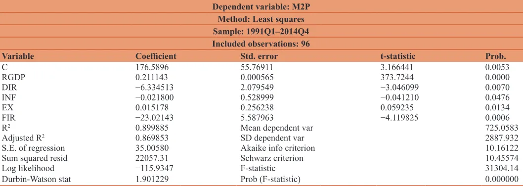
the result of the multiple regressions.
The coefficient on the real income variable indicates that the long run income elasticity for real broad money is 0.2111. This means that
a 1% increase in real income increases the demand for real money
balances by 0.21%. The long run income elasticity of less than one supports the argument of several studies that financial development
and liberalization, technological improvements in payment system, creation of money substitutes and improved economic stability should decrease the income elasticity of money demand (Owoye
and Onafowora, 2007; p.8). This result is in conformity with the findings of Nduka et al. (2013), Iyoboyi and Pedro (2013) for Nigeria and Mansaray and Swaray (2012) for Sierra Leone.
The results show that the interest rate coefficient carries a negative sign and is statistically significant. This implies that in the long
run, the demand for broad money balances remain dependent on the domestic interest rate. Thus, the interest rate is a good proxy of
the opportunity cost of holding money and has a significant effect on the demand for broad money in Nigeria. The coefficient of the domestic interest rate follows Friedman’s quantity theory of money and is consistent with the contributions of Nduka et al. (2013) and Akinlo (2006) for Nigeria. This result is in contrast to Imimole and Uniamikogbo (2014), Onafowora and Owoye (2008) for Nigeria, Kapingura (2014) for South Africa and Abdulkheir (2013) for Saudi Arabia whose empirical results showed that the coefficient
of domestic interest rate is positively related to real money demand.
The inflation rate elasticity is negative (−0.0218) and significant, supporting Friedman’s theoretical expectations. This means that the higher the inflation rate, the lower the demand for broad money in Nigeria i.e a 1% increase in inflation decreases demand for real money balances by 0.02% in the long run. Inflation growth
will lead to increased return on alternative forms of assets such
as equity holding (shares), investment in land and real estate and
commodities, which will reduce demand for naira. This suggest that
Table 1: ADF unit root tests from M2 money demand function
Variables At level with constant, no trend At first difference with constant, no trend
ADF statistics 5% critical value ADF statistics 5% critical value
LOGM2P −3.83 −2.9980 −1.0429 −3.0048
LOGRGDP −3.13 −2.9980 −0.7476 −3.0048
LOGDIR −2.02 −2.9980 −5.3786 −3.0048
LOGINF −2.38 −3.0048 −4.6004 −3.0048
LOGEX −2.06 −2.9980 −4.6551 −3.0048
LOGFIR 2.44 −3.0299 −3.3833 −3.0048
Source: Researcher’s Eview result. ADF: Augmented Dickey Fuller
Table 2: Regression result
Dependent variable: M2P Method: Least squares Sample: 1991Q1–2014Q4 Included observations: 96
Variable Coefficient Std. error t-statistic Prob.
C 176.5896 55.76911 3.166441 0.0053
RGDP 0.211143 0.000565 373.7244 0.0000
DIR −6.334513 2.079549 −3.046099 0.0070
INF −0.021800 0.528999 −0.041210 0.0476
EX 0.015178 0.256238 0.059235 0.0134
FIR −23.02143 5.587963 −4.119825 0.0006
R2 0.899885 Mean dependent var 725.0583
Adjusted R2 0.869853 SD dependent var 2887.932
S.E. of regression 35.00580 Akaike info criterion 10.16122
Sum squared resid 22057.31 Schwarz criterion 10.45574
Log likelihood −115.9347 F-statistic 31304.14
Durbin-Watson stat 1.901229 Prob (F-statistic) 0.000000
the hedging effect of inflation on money demand is greater than the investment effect. This finding is in consonance with many studies like Mansaray and Swaray (2012) for Sierra Leone, Imimole and Uniamikogbo (2014) for Nigeria, Kjosevski (2013) for Macedonia, Dritsakis (2012) for Hungary and Sharifi-Renani (2007) for Iran. The result is at variance with Abdulkheir (2013) for Saudi Arabia whose findings indicated a positive and statistically significant long run relation between the inflation rate and money demand.
There is also a positive and statistically significant effect of
exchange rate on real broad money demand supporting the wealth effect argument in the literature. This is consistent with theory that predicts that an increase in exchange rate can be perceived as an increase in wealth, leading to a rise in the demand for domestic money. Depreciation of the exchange rate increases the external value of the domestic currency in foreign assets. Thus, wealth holders who perceive this as an increase in their wealth tend to convert a portion of their foreign assets to domestic assets in a
bid to maintain a fixed share of their wealth that are invested in domestic currency (Mansaray and Swaray, 2012. p. 81). The positive coefficient of exchange rate in Nigeria is in conformity with the findings of Akinlo (2006), Imimole and Uniamikogbo (2014) for Nigeria, Sharifi-Renani (2007) for Iran and Mansaray and Swaray (2012) for Sierra Leone. It also contradicts the findings of Kapingura (2014) for South Africa, Onafowara and Owoye (2004), and Nduka et al. (2013) for Nigeria as they attributed the negative coefficient of the exchange rate depreciation to the
existence of currency substitution in Nigeria.
The foreign interest rate coefficient is negative and statistically significant. A 1% rise in foreign interest rate may lead to 23.02%
fall in the demand for real money balances. This result is supportive of the portfolio balance argument of capital mobility and highlights the importance of foreign effects in explaining the demand for real
broad money in Nigeria during the sample period. This finding is in consonance with the studies of Onafowora and Owoye (2008) and Imimole and Uniamikogbo (2014) for Nigeria. The result is in contrast to Nduka et al. (2013) who did not support the argument of capital mobility because the coefficient of foreign interest rate was positively related to real money demand for the period of 1986–2011 in Nigeria.
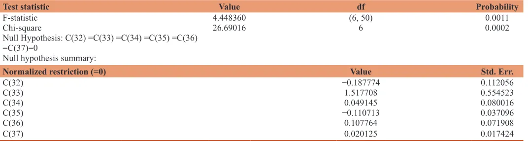
To investigate the presence of long run relationship among the
variables, bounds testing procedure was used (Table 3).
The value of our F-statistic is 4.44 and we have (K+1) = 6 variables (M2/P, RGDP, DIR, INF, EX and FIR) in our model. The lower and upper bounds for the F-test statistic at 5% significance levels are 2.81 and 3.76 respectively (Pesaran et al., 2001. p. 300). We did not constrain
the intercept of our model and there is linear trend term included.
As the F-statistic value of 4.44 exceeds the upper bound of
3.76 at the 5% significance level, we can conclude that there is
cointegrating relationship between real money demand, real GDP,
domestic interest rate, inflation rate, exchange rate and foreign
interest rate in Nigeria. The calculated F-statistics clearly rejects
null hypothesis of no cointegration at 5% level of significance. This is consistent with several studies like Bhatta (2013) for Nepal and Dritsakis (2011) for Hungary. This findings is at variance with Akinlo (2006) over the period 1970:1–2002:4 for Nigeria whose
result showed that there is no strong evidence of cointegration and
Sheefeni (2013) who found that there is no cointegration between
real money balances and the selected macroeconomic variables in
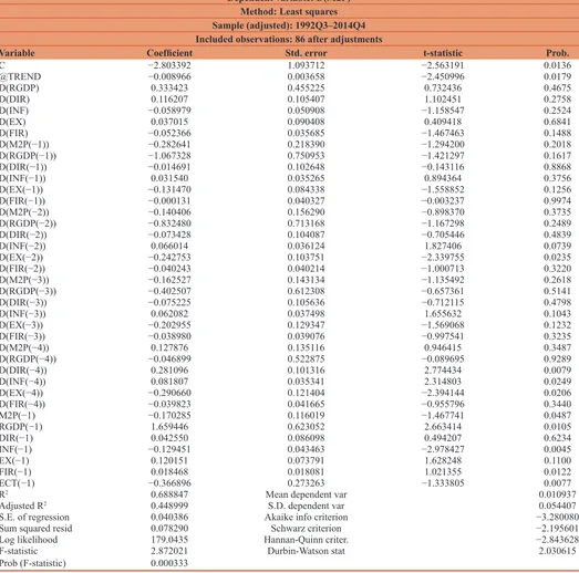
Namibia. Table 4 shows the ARDL error correction model.
The presence of a cointegrating relationship among real money balances and its explanatory variables validates the estimation of
a short run dynamic model. The coefficient of the error correction
term, ECTt−1 is negative and significant. The ECT measures the speed of adjustment towards equilibrium. The coefficient of the feedback parameter is −0.3669. This means reversion speed is
relatively high. This implies that if there are departures from equilibrium in the previous period, the departures are reduced by
about 36% in the current period. When real broad money balances
deviate in the short run from real income, domestic interest rate,
inflation rate, exchange rate and foreign interest rate, its speed of
adjustment to long run equilibrium is about 36% per quarter and
is statistically significant.
This correction speed of adjustment is comparatively more
consistent than the findings in other studies such as: 31% in
Vietnam, 16% in Iran (Sharifi-Renani, 2007), 13% in Greece (Dritsakis, 2011), 6% in Nigeria (Owoye and Onafowora, 2007) and 4.9% in Cambodia.
The goodness of fit for the short run ARDL model is 68% and the adjusted R2 is 44%. The adjusted R2 of the error correction model is rather low but it does not significantly affect our results since
Table 3: Wald test for cointegration
Test statistic Value df Probability
F-statistic 4.448360 (6, 50) 0.0011
Chi-square 26.69016 6 0.0002
Null Hypothesis: C(32) =C(33) =C(34) =C(35) =C(36) =C(37)=0
Null hypothesis summary:
Normalized restriction (=0) Value Std. Err.
C(32) −0.187774 0.112056
C(33) 1.517708 0.554523
C(34) 0.049145 0.080016
C(35) −0.110713 0.037096
C(36) 0.107764 0.071908
C(37) 0.020125 0.017424
the variables are in the difference form. Durbin Watson statistic of 2.03 is indicative of the absence of autocorrelation.
This model with 4 period lags based on SBC was selected since the SBC is parsimonious as it uses minimum acceptable lag while selecting the lag length and avoids unnecessary loss of degrees of
freedom (Bhatta, 2013. p. 14). The lag selection result is displayed
Table 5.
Finally, the stability of the long run coefficients together with
the short run dynamics was examined. The CUSUM and the
CUSUMSQ tests were applied (Figures 1 and 2).
Finally, the CUSUM and CUSUMSQ indicate that the estimated short run dynamics and long run parameters of the money demand function are stable, since the plots of these graphs are confined
within the 5% critical bounds of parameter stability. Thus, a stable real broad money demand function exists in Nigeria over the entire period of the analysis.
5. CONCLUSIONS
Given the importance attached to money demand and its stability in the success or failure of monetary policy the results of this study reveal that a cointegrating relationship exist between the Table 4: Error correction model result
Dependent variable: D(M2P) Method: Least squares Sample (adjusted): 1992Q3–2014Q4 Included observations: 86 after adjustments
Variable Coefficient Std. error t-statistic Prob.
C −2.803392 1.093712 −2.563191 0.0136
@TREND −0.008966 0.003658 −2.450996 0.0179
D(RGDP) 0.333423 0.455225 0.732436 0.4675
D(DIR) 0.116207 0.105407 1.102451 0.2758
D(INF) −0.058979 0.050908 −1.158547 0.2524
D(EX) 0.037015 0.090408 0.409418 0.6841
D(FIR) −0.052366 0.035685 −1.467463 0.1488
D(M2P(−1)) −0.282641 0.218390 −1.294200 0.2018
D(RGDP(−1)) −1.067328 0.750953 −1.421297 0.1617
D(DIR(−1)) −0.014691 0.102648 −0.143116 0.8868
D(INF(−1)) 0.031540 0.035265 0.894364 0.3756
D(EX(−1)) −0.131470 0.084338 −1.558852 0.1256
D(FIR(−1)) −0.000131 0.040327 −0.003237 0.9974
D(M2P(−2)) −0.140406 0.156290 −0.898370 0.3735
D(RGDP(−2)) −0.832480 0.713168 −1.167298 0.2489
D(DIR(−2)) −0.073428 0.104087 −0.705446 0.4839
D(INF(−2)) 0.066014 0.036124 1.827406 0.0739
D(EX(−2)) −0.242753 0.103751 −2.339755 0.0235
D(FIR(−2)) −0.040243 0.040214 −1.000713 0.3220
D(M2P(−3)) −0.162527 0.143134 −1.135492 0.2618
D(RGDP(−3)) −0.402507 0.612308 −0.657361 0.5141
D(DIR(−3)) −0.075225 0.105636 −0.712115 0.4798
D(INF(−3)) 0.062082 0.037498 1.655632 0.1043
D(EX(−3)) −0.202955 0.129347 −1.569068 0.1232
D(FIR(−3)) −0.038980 0.039076 −0.997541 0.3235
D(M2P(−4)) 0.127876 0.135116 0.946415 0.3487
D(RGDP(−4)) −0.046899 0.522875 −0.089695 0.9289
D(DIR(−4)) 0.281096 0.101316 2.774434 0.0079
D(INF(−4)) 0.081807 0.035341 2.314803 0.0249
D(EX(−4)) −0.290660 0.121404 −2.394144 0.0206
D(FIR(−4)) −0.039823 0.041665 −0.955796 0.3440
M2P(−1) −0.170285 0.116019 −1.467741 0.0487
RGDP(−1) 1.659446 0.623052 2.663414 0.0105
DIR(−1) 0.042550 0.086098 0.494207 0.6234
INF(−1) −0.129451 0.043463 −2.978427 0.0045
EX(−1) 0.120151 0.073791 1.628248 0.1100
FIR(−1) 0.018468 0.018081 1.021355 0.0122
ECT(−1) −0.366896 0.273263 −1.333805 0.0077
R2 0.688847 Mean dependent var 0.010937
Adjusted R2 0.448999 S.D. dependent var 0.054407
S.E. of regression 0.040386 Akaike info criterion −3.280080
Sum squared resid 0.078290 Schwarz criterion −2.195601
Log likelihood 179.0435 Hannan-Quinn criter. −2.843628
F-statistic 2.872021 Durbin-Watson stat 2.030615
Prob (F-statistic) 0.000333
real broad money, real income, domestic interest rate, inflation
rate, exchange rate and foreign interest rate. Furthermore, the
CUSUM and CUSUMSQ test also confirmed the stability of the
long-run money demand function. However, monetary targeting is still relevant in setting monetary policy framework in Nigeria.
REFERENCES
Abdulkheir, A.Y. (2013), An analytical study of the demand for money in Saudi Arabia. International Journal of Economics and Finance, 5(4), 31-38.
Achsani, N.A. (2010), Stability of money demand in an emerging market economy: An error correction and ARDL model for Indonesia. Research Journal of International Studies, 13, 83-91. Available from: http://www.pascaie.ipb.ac.id›doc›jurnal7.
Akinlo, A.E. (2006), The stability of money demand in Nigeria: An autoregressive distributed lag approach. Journal of Policy Modeling, 28(4), 445-452.
Bhatta, S.R. (2013), Stability of money demand in Nepal. Banking Journal, 3(1), 1-27.
Brown, R.L., Durbin, J., Evans, J.M. (1975), Techniques for testing the constancy of regression relations over time. Journal of the Royal Statistical Society, 37, 149-192. Available from: http://www.ftp.uic. edu›brown_durbin_evans.
Dagher, J., Kovanen, A. (2011), On the Stability of Money Demand in Ghana: A Bounds Testing Approach. IMF Working Paper, WP/11/273 No. 1-18. Available from: https://www.imf.org›pubs›2011. Dharmadasa, C., Nakanishi, M. (2013), Demand for Money in Sri
Lanka: ARDL Approach to Co-integration. Proceedings of the 3rd International Conference on Humanities, Geography and Economics, Bali, Indonesia: Planetary Scientific Research Centre. p143-147. Available from: http://www.psrcentre. org›images›extraimages.
Doguwa, S.I., Olowofeso, O.E., Uyaebo, S.O., Adamu, I., Bada, A.S. (2014), Structural breaks, cointegration and demand for money in Nigeria. CBN Journal of Applied Statistics, 5(1), 15-33. Available from: http://www.cenbank.org.
Dritsakis, N. (2011), Demand for money in Hungary: An ARDL approach. Review of Economics and Finance, 1, 1-16.
Dritsaki, C., Dritsaki, M. (2012), The stability of money demand: Evidence from Turkey. The IUP Journal of Bank Management, 9(4), 7-28. Available from: http://www.ssrn.com.
Imimole, B., Uniamikogbo, S.O. (2014), Testing for the stability of money demand function in Nigeria. Journal of Economics and Sustainable Development, 5(6), 123-130. Available from: http://www.iiste. org›JEDS›article›viewfile.
Table 5: Lag selection result
VAR lag order selection criteria Endogenous variables: D(M2P)
Exogenous variables: C (M2P(-1)) D(RGDP(-1)) D(DIR(-1)) D(INF(-1)) D(EX(-1)) D(FIR(-1)) Sample: 1991Q1–2014Q4
Included observations: 79
Lag LogL LR FPE AIC SC HQ
0 116.7427 NA 0.003640 −2.778295 −2.568344 −2.694182
1 118.2558 2.719806 0.003594 −2.791286 −2.551342 −2.695157
2 119.6633 2.494376 0.003558 −2.801603 −2.531666 −2.693458
3 120.3597 1.216365 0.003587 −2.793915 −2.493985 −2.673754
4 126.7108 10.93367* 0.003134* −2.929388* −2.599465* −2.797211*
5 127.0553 0.584226 0.003188 −2.912792 −2.552875 −2.768598
6 127.6435 0.982796 0.003224 −2.902366 −2.512457 −2.746156
7 127.6793 0.058933 0.003306 −2.877956 −2.458054 −2.709730
8 128.9018 1.980733 0.003290 −2.883589 −2.433693 −2.703347
9 129.2756 0.596219 0.003346 −2.867736 −2.387848 −2.675478
10 129.5565 0.440897 0.003412 −2.849531 −2.339650 −2.645257
11 130.1028 0.843740 0.003456 −2.838046 −2.298172 −2.621756
12 130.2465 0.218179 0.003536 −2.816366 −2.246499 −2.588060
*İndicates lag order selected by the criterion. LR: Sequential modified LR test statistic (each test at 5% level), FPE: Final prediction error, AIC: Akaike information criterion, SC: Schwarz information criterion, HQ: Hannan-Quinn information criterion. Source: Researcher’s Eview result
Source: Researcher’s Eview result
Figure 1: Plot of cumulative sum of recursive residuals
Figure 2: Plot of cumulative sum of squares of recursive residuals
Iyoboyi, M., Pedro, L.M. (2013), The demand for money in Nigeria: Evidence from bounds testing approach. Business and Economics Journal, 2013(76), 1-13. Available from: http://www.astonjournals. com/bej.
Kapingura, F.M. (2014), The stability of the money demand function in South Africa: A VAR-based approach. International Business and Economics Research Journal, 13, 1471-1482. Available from: http:// connection.ebscohost.com›article.
Kiptui, M.C. (2014), Some empirical evidence on the stability of money demand in Kenya. International Journal of Economics and Financial Issues, 4(4), 849. Available from: http://www.econjournals. com›viewFiles›pdf.
Kjosevski, J. (2013), The determinants and stability of money demand in the Republic of Macedonia. Proceedings of Rijeka faculty of economics. Journal of Economics and Business, 31(1), 35-54. Kumar, P. (2014), The determinants and stability of money demand in
India. Online International Interdisciplinary Research Journal, 4, 80-92. Available from: http://www.oiirj.org›nov2014-special-issue. Kumar, S., Webber, D.J., Fargher, S. (2010), Money Demand Stability:
A Case Study of Nigeria. MPRA Paper 26074, University Library of Munich, Germany. Available from: https://www.mpra.ub.uni-muenchen.de/id/eprint/26074.
Lungu, M., Simwaka, K., Chiumia, A., Palamuleni, A., Jombo, W. (2012), Money demand function for malawi-ımplications for monetary policy conduct. Banks and Bank systems, 7(1), 50-63. Available from: https://www.rbm.mw.
Mansaray, M., Swaray, S. (2012), Financial liberalization, monetary policy and money demand in Sierra Leone. Journal of Monetary and Economic Integration, 12(2), 62-90. Available from: http://www. wami-imao.org›files›journals.
Mishkin, F.S. (2010), The Economics of Money, Banking and Financial
Markets. New York: Addison-Wesley Publishing Company. Nduka, E.K., Chukwu, J.O., Nwakaire, O.N. (2013), Stability of demand
for money in Nigeria. Asian Journal of Business and Economics, 3(3.4), 1-11. Available from: http://www.onlineresearchjournals.com. Omer, M. (2010), Stability of Money Demand Function in Pakistan.
SBP Working Paper Series, 36, 1-30. Available from: http://www. sbp.org.pk.
Onafowora, O., Owoye, O. (2008), Exchange rate volatility and export growth in Nigeria. Applied Economics, 40(12), 1547-1556. Owoye, O., Onafowora, O.A. (2007), M2 targeting, money demand and
real GDP growth in Nigeria: Do rules apply? Journal of Business and Public Affairs, 1(2), 1-20. Available from: https://www.econbiz.de. Özcalik, M. (2014), Money demand function in Turkey: An ARDL
approach. Journal of Socialand Economic Research, 14 (27), 360-373. Available from: http://www.sead.selcuk.edu.tr.
Pesaran, M.H., Shin, Y., Smith, R.J. (2001), Bounds testing approaches to the analysis of level relationships. Journal of Applied Econometrics, 16, 289-326.
Sharifi-Renani, H. (2007), Demand for Money in Iran: An ARDL Approach. Available from: http://www.mpra.ub.uni-muenchen. de/8224/MPRA Paper No.8224,posted 16. [Last accessed on 2008 April 02].
Sheefeni, J.P.S. (2013), Demand for money in Namibia: An ARDL bounds testing approach. Asian Journal of Business and Management, 1(3), 65-71. Available from: http://www.ajouronline.com›journal=AJMB. Sober, M. (2013), Estimating a function of real demand for money in
Pakistan: An application of bounds testing approach to cointegration. International Journal of Computer Application, 79(5), 32-50. Suliman, S.Z., Dafaalla, H.A. (2011), An econometric analysis of money
APPENDIX
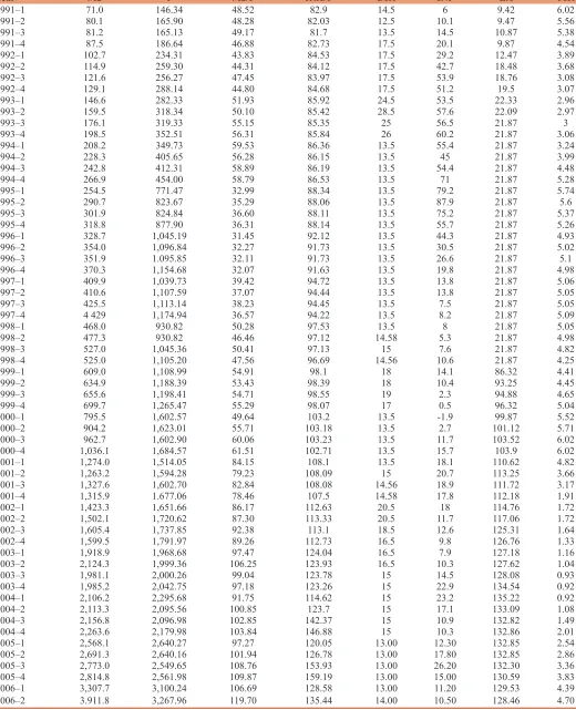
Table A1: Quantum values of selected varıables(Contd...)
Year M2 P M2/P RGDP DIR INF EX FIR
1991–1 71.0 146.34 48.52 82.9 14.5 6 9.42 6.02
1991–2 80.1 165.90 48.28 82.03 12.5 10.1 9.47 5.56
1991–3 81.2 165.13 49.17 81.7 13.5 14.5 10.87 5.38
1991–4 87.5 186.64 46.88 82.73 17.5 20.1 9.87 4.54
1992–1 102.7 234.31 43.83 84.53 17.5 29.2 12.47 3.89
1992–2 114.9 259.30 44.31 84.12 17.5 42.7 18.48 3.68
1992–3 121.6 256.27 47.45 83.97 17.5 53.9 18.76 3.08
1992–4 129.1 288.14 44.80 84.68 17.5 51.2 19.5 3.07
1993–1 146.6 282.33 51.93 85.92 24.5 53.5 22.33 2.96
1993–2 159.5 318.34 50.10 85.42 28.5 57.6 22.09 2.97
1993–3 176.1 319.33 55.15 85.35 25 56.5 21.87 3
1993–4 198.5 352.51 56.31 85.84 26 60.2 21.87 3.06
1994–1 208.2 349.73 59.53 86.36 13.5 55.4 21.87 3.24
1994–2 228.3 405.65 56.28 86.15 13.5 45 21.87 3.99
1994–3 242.8 412.31 58.89 86.19 13.5 54.4 21.87 4.48
1994–4 266.9 454.00 58.79 86.53 13.5 71 21.87 5.28
1995–1 254.5 771.47 32.99 88.34 13.5 79.2 21.87 5.74
1995–2 290.7 823.67 35.29 88.06 13.5 87.9 21.87 5.6
1995–3 301.9 824.84 36.60 88.11 13.5 75.2 21.87 5.37
1995–4 318.8 877.90 36.31 88.14 13.5 55.7 21.87 5.26
1996–1 328.7 1,045.19 31.45 92.12 13.5 44.3 21.87 4.93
1996–2 354.0 1,096.84 32.27 91.73 13.5 30.5 21.87 5.02
1996–3 351.9 1.095.85 32.11 91.73 13.5 26.6 21.87 5.1
1996–4 370.3 1,154.68 32.07 91.63 13.5 19.8 21.87 4.98
1997–1 409.9 1,039.73 39.42 94.72 13.5 13.8 21.87 5.06
1997–2 410.6 1,107.59 37.07 94.44 13.5 13.8 21.87 5.05
1997–3 425.5 1,113.14 38.23 94.45 13.5 7.5 21.87 5.05
1997–4 4 429 1,174.94 36.57 94.22 13.5 8.2 21.87 5.09
1998–1 468.0 930.82 50.28 97.53 13.5 8 21.87 5.05
1998–2 477.3 930.82 46.46 97.12 14.58 5.3 21.87 4.98
1998–3 527.0 1,045.36 50.41 97.13 15 7.6 21.87 4.82
1998–4 525.0 1,105.20 47.56 96.69 14.56 10.6 21.87 4.25
1999–1 609.0 1,108.99 54.91 98.1 18 14.1 86.32 4.41
1999–2 634.9 1,188.39 53.43 98.39 18 10.4 93.25 4.45
1999–3 655.6 1,198.41 54.71 98.55 19 2.3 94.88 4.65
1999–4 699.7 1,265.47 55.29 98.07 17 0.5 96.32 5.04
2000–1 795.5 1,602.57 49.64 103.2 13.5 -1.9 99.87 5.52
2000–2 904.2 1,623.01 55.71 103.18 13.5 2.7 101.12 5.71
2000–3 962.7 1,602.90 60.06 103.23 13.5 11.7 103.52 6.02
2000–4 1,036.1 1,684.57 61.51 102.71 13.5 15.7 103.9 6.02
2001–1 1,274.0 1,514.05 84.15 108.1 13.5 18.1 110.62 4.82
2001–2 1,263.2 1,594.28 79.23 108.09 15 20.7 113.25 3.66
2001–3 1,327.6 1,602.70 82.84 108.08 14.56 18.9 111.72 3.17
2001–4 1,315.9 1.677.06 78.46 107.5 14.58 17.8 112.18 1.91
2002–1 1,423.3 1,651.66 86.17 112.63 20.5 18 114.76 1.72
2002–2 1,502.1 1,720.62 87.30 113.33 20.5 11.7 117.06 1.72
2002–3 1,605.4 1,737.85 92.38 113.1 18.5 12.6 125.31 1.64
2002–4 1,599.5 1,791.97 89.26 112.73 16.5 9.8 126.76 1.33
2003–1 1,918.9 1,968.68 97.47 124.04 16.5 7.9 127.18 1.16
2003–2 2,124.3 1,999.36 106.25 123.93 16.5 10.3 127.62 1.04
2003–3 1,981.1 2,000.26 99.04 123.78 15 14.5 128.08 0.93
2003–4 1,985.2 2,042.75 97.18 123.26 15 22.9 134.54 0.92
2004–1 2,106.2 2,295.68 91.75 114.62 15 23.2 135.22 0.92
2004–2 2,113.3 2,095.56 100.85 123.7 15 17.1 133.09 1.08
2004–3 2,156.8 2,096.98 102.85 142.37 15 10.9 132.82 1.49
2004–4 2,263.6 2,179.98 103.84 146.88 15 10.3 132.86 2.01
2005–1 2,568.1 2,640.27 97.27 120.05 13.00 12.30 132.85 2.54
2005–2 2,691.3 2,640.16 101.94 126.78 13.00 17.80 132.85 2.86
2005–3 2,773.0 2,549.65 108.76 153.93 13.00 26.20 132.30 3.36
2005–4 2,814.8 2,561.98 109.87 159.19 13.00 15.00 130.59 3.83
2006–1 3,307.7 3,100.24 106.69 128.58 13.00 11.20 129.53 4.39
Year M2 P M2/P RGDP DIR INF EX FIR
2006–3 4,320.7 3,068.63 140.80 162.50 14.00 4.30 128.33 4.91
2006–4 4,027.9 3,051.16 132.01 169.30 10.00 7.50 128.29 4.90
2007–1 4,798.3 3,491.67 137.42 135.77 10.00 6.70 128.23 4.98
2007–2 5,116.2 3,399.92 150.48 142.76 8.00 5.10 127.65 4.74
2007–3 5,672.6 3,192.04 177.71 173.07 8.00 4.40 126.58 4.30
2007–4 5,809.8 3,032.71 191.57 182.62 9.00 5.40 120.87 3.39
2008–1 7,998.2 3,896.61 205.26 142.07 9.50 8.10 118.04 2.04
2008–2 7,948.4 3,791.71 209.63 150.86 10.25 10.00 117.84 1.63
2008–3 8,960.3 3,518.04 254.70 183.68 9.75 13.10 117.75 1.49
2008–4 9,166.8 3,363.27 272.56 195.59 9.75 14.80 120.65 0.30
2009–1 8,997.8 3,660.24 245.83 149.19 9.75 14.30 146.88 0.21
2009–2 9,077.0 3,622.86 250.55 162.10 8.00 12.50 147.76 0.17
2009–3 9,458.5 3,353.10 282.08 197.08 6.00 10.80 150.90 0.16
2009–4 10,780.6 3,253.72 331.33 210.60 6.00 12.60 149.97 0.06
2010–1 11,023.3 4,638.18 237.66 160.12 6.00 14.90 149.94 0.11
2010–2 10,845.5 4,603.11 235.61 174.73 6.00 14.00 150.13 0.15
2010–3 11,224.8 4,256.03 263.74 212.77 6.25 13.40 150.47 0.16
2010–4 11,525.5 4,135.99 278.66 228.71 6.25 12.60 150.65 0.14
2011–1 11,653.6 4,994.57 233.33 171.27 7.50 12.00 152.00 0.13
2011–2 12,172.1 5,028.32 242.07 187.83 8.00 11.30 154.42 0.05
2011–3 12,618.1 4,314.28 292.47 228.45 9.25 9.60 153.28 0.02
2011–4 13.303.5 3,877.04 343.14 246.45 12.00 10.40 155.75 0.01
2012–1 13,271.0 5,020.25 264.35 181.12 12 12.2 157.95 0.07
2012–2 13,483.1 4,924.26 273.81 199.83 12.00 12.8 157.35 0.09
2012–3 14,065.3 4,508.40 311.98 243.26 12.00 11.9 157.38 0.1
2012–4 15,483.8 4,017.67 385.39 263.68 12.00 12 157.32 0.09
2013–1 15,669.2 4,892.10 320.30 194.06 12.00 9 157.3 0.09
2013–2 15,593.2 4,809.46 324.22 212.18 12.00 8.8 157.31 0.05
2013–3 14,362.5 4,297.28 334.22 259.84 12.00 8.3 157.32 0.03
2013–4 15,689.0 4,060.20 386.41 284.03 12.00 7.9 157.32 0.06
2014–1 17,732.9 130.64 13,573.87 15438.68 12.00 7.8 157.3 0.05
2014–2 16,171.6 135.13 11,967.44 16084.62 12.00 8 157.29 0.03
2014–3 16,814.5 131.20 12,815.93 17479.13 12.00 8.3 157.29 0.03
2014–4 18,927.8 133.36 14,193.01 18150.36 13 8 162.33 0.02
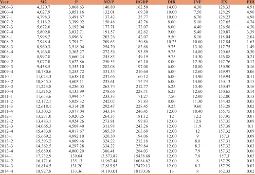
Sources: Central Bank of Nigeria Statistical Bulletin, December, 2014. IMF World Economic Outlook Database, April, 2015 and Researcher’s Computations. M2: Nominal M2 money stock, P: Implicit price deflator, M2/P: Real M2 money balances (N’ Billion) is the dependent variable, RGDP: Real income (N’ Billion), DIR: Domestic interest rate (%), INF: Inflation rate (%), EX: Expected exchange rate (N/$1.00), FIR: Foreign interest rate (%) are the independent variables. 2014 rebased gross domestic product and implicit price deflator figures at 2010 constant basic prices
Year LOGM2P LOGRGDP LOG(DIR) LOGINF LOGEX LOGFIR
1991–1 1.69 1.92 1.16 0.78 0.97 0.78
1991–2 1.68 1.91 1.10 1.00 0.98 0.75
1991–3 1.69 1.91 1.13 1.16 1.04 0.73
1991–4 1.67 1.92 1.24 1.30 0.99 0.66
1992–1 1.64 1.93 1.24 1.47 1.10 0.59
1992–2 1.65 1.92 1.24 1.63 1.27 0.57
1992–3 1.68 1.92 1.24 1.73 1.27 0.49
1992–4 1.65 1.93 1.24 1.71 1.29 0.49
1993–1 1.72 1.93 1.39 1.73 1.35 0.47
1993–2 1.70 1.93 1.45 1.76 1.34 0.47
1993–3 1.74 1.93 1.40 1.75 1.34 0.48
1993–4 1.75 1.93 1.41 1.78 1.34 0.49
1994 –1 1.77 1.94 1.13 1.74 1.34 0.51
1994–2 1.75 1.94 1.13 1.65 1.34 0.60
1994–3 1.77 1.94 1.13 1.74 1.34 0.65
1994–4 1.77 1.94 1.13 1.85 1.34 0.72
1995–1 1.52 1.95 1.13 1.90 1.34 0.76
1995–2 1.55 1.94 1.13 1.94 1.34 0.75
1995–3 1.56 1.95 1.13 1.88 1.34 0.73
1995–4 1.56 1.95 1.13 1.75 1.34 0.72
1996–1 1.50 1.96 1.13 1.65 1.34 0.69
1996–2 1.51 1.96 1.13 1.48 1.34 0.70
1996–3 1.51 1.96 1.13 1.42 1.34 0.71
1996–4 1.51 1.96 1.13 1.30 1.34 0.70
1997–1 1.60 1.98 1.13 1.14 1.34 0.70
1997–2 1.57 1.98 1.13 1.14 1.34 0.70
1997–3 1.58 1.98 1.13 0.88 1.34 0.70
1997–4 1.56 1.97 1.13 0.91 1.34 0.71
1998–1 1.70 1.99 1.13 0.90 1.34 0.70
1998–2 1.67 1.99 1.16 0.72 1.34 0.70
1998–3 1.70 1.99 1.18 0.88 1.34 0.68
1998–4 1.68 1.99 1.16 1.03 1.34 0.63
1999–1 1.74 1.99 1.26 1.15 1.94 0.64
1999–2 1.73 1.99 1.26 1.02 1.97 0.65
1999–3 1.74 1.99 1.28 0.36 1.98 0.67
1999–4 1.74 1.99 1.23 –0.30 1.98 0.70
2000–1 1.70 2.01 1.13 0.28 2.00 0.74
2000–2 1.75 2.01 1.13 0.43 2.00 0.76
2000–3 1.78 2.01 1.13 1.07 2.02 0.78
2000–4 1.79 2.01 1.13 1.20 2.02 0.78
2001–1 1.93 2.03 1.13 1.26 2.04 0.68
2001–2 1.90 2.03 1.18 1.32 2.05 0.56
2001–3 1.92 2.03 1.16 1.28 2.05 0.50
2001–4 1.89 2.03 1.16 1.25 2.05 0.28
2002–1 1.94 2.05 1.31 1.26 2.06 0.24
2002–2 1.94 2.05 1.31 1.07 2.07 0.24
2002–3 1.97 2.05 1.27 1.10 2.10 0.21
2002–4 1.95 2.05 1.22 0.99 2.10 0.12
2003–1 1.99 2.09 1.22 0.90 2.10 0.06
2003–2 2.03 2.09 1.22 1.01 2.11 0.02
2003–3 2.00 2.09 1.18 1.16 2.11 –0.03
2003–4 1.99 2.09 1.18 1.36 2.13 –0.04
2004–1 1.96 2.06 1.18 1.37 2.13 –0.04
2004–2 2.00 2.09 1.18 1.23 2.12 0.03
2004–3 2.01 2.15 1.18 1.04 2.12 0.17
2004–4 2.02 2.17 1.18 1.01 2.12 0.30
2005–1 1.99 2.08 1.11 1.09 2.12 0.40
2005–2 2.01 2.10 1.11 1.25 2.12 0.46
2005–3 2.04 2.19 1.11 1.42 2.12 0.53
2005–4 2.04 2.20 1.11 1.18 2.12 0.58
2006–1 2.03 2.11 1.11 1.05 2.11 0.64
2006–2 2.08 2.13 1.15 1.02 2.11 0.67
2006–3 2.15 2.21 1.15 0.63 2.11 0.69
2006–4 2.12 2.23 1.00 0.88 2.11 0.69
2007–1 2.14 2.13 1.00 0.83 2.11 0.70
Table A2: Logged values of selected varıables
Table A3: Correlation matrix
M2P RGDP DIR INF EX FIR
M2P 1.000000
RGDP 0.941963 1.000000
DIR −0.412069 −0.243983 1.000000
INF −0.325986 −0.262345 0.269213 1.000000
EX 0.623110 0.429846 −0.436834 −0.477309 1.000000
FIR −0.796329 −0.645755 0.470939 0.196478 −0.595517 1.000000
Source: Researcher’s Eview result
Table A4: Heteroscedasticity test for the first hypothesis White heteroskedasticity test
F-statistic 0.929882 Probability 0.618034
Obs*R2 20.66630 Probability 0.417002
Source: Researcher’s Eview result
Table A5: Autocorrelation test Breusch-Godfrey serial correlation LM test
F-statistic 2.953030 Probability 0.080993
Obs*R2 6.470604 Probability 0.113480
Durbin-Watson stat 1.901229
Source: Researcher’s Eview result
Year LOGM2P LOGRGDP LOG(DIR) LOGINF LOGEX LOGFIR
2007–2 2.18 2.15 0.90 0.71 2.11 0.68
2007–3 2.25 2.24 0.90 0.64 2.10 0.63
2007–4 2.28 2.26 0.95 0.73 2.08 0.53
2008–1 2.31 2.15 0.98 0.91 2.07 0.31
2008–2 2.32 2.18 1.01 1.00 2.07 0.21
2008–3 2.41 2.26 0.99 1.12 2.07 0.17
2008–4 2.44 2.29 0.99 1.17 2.08 −0.52
2009–1 2.39 2.17 0.99 1.16 2.17 −0.68
2009–2 2.40 2.21 0.90 1.10 2.17 −0.77
2009–3 2.45 2.29 0.78 1.03 2.18 −0.80
2009–4 2.52 2.32 0.78 1.10 2.18 −1.22
2010–1 2.38 2.20 0.78 1.17 2.18 −0.96
2010–2 2.37 2.24 0.78 1.15 2.18 −0.82
2010–3 2.42 2.33 0.80 1.13 2.18 −0.80
2010–4 2.45 2.36 0.80 1.10 2.18 −0.85
2011–1 2.37 2.23 0.88 1.08 2.18 −0.89
2011–2 2.38 2.27 0.90 1.05 2.19 −1.30
2011–3 2.47 2.36 0.97 0.98 2.19 −1.70
2011–4 2.54 2.39 1.08 1.02 2.19 −2.00
2012–1 2.42 2.26 1.08 1.09 2.20 −1.15
2012–2 2.44 2.30 1.08 1.11 2.20 −1.05
2012–3 2.49 2.39 1.08 1.08 2.20 −1.00
2012–4 2.59 2.42 1.08 1.08 2.20 −1.05
2013–1 2.51 2.29 1.08 0.95 2.20 −1.05
2013–2 2.51 2.33 1.08 0.94 2.20 −1.30
2013–3 2.52 2.41 1.08 0.92 2.20 −1.52
2013–4 2.59 2.45 1.08 0.90 2.20 −1.22
2014–1 4.13 4.19 1.08 0.89 2.20 −1.30
2014–2 4.08 4.21 1.08 0.90 2.20 −1.52
2014–3 4.11 4.24 1.08 0.92 2.20 −1.52
2014–4 4.15 4.26 1.11 0.90 2.21 −1.70
Table A6: ADFF unit root tests from M2 money demand function
Variables At level with constant, no trend At first difference with constant, no trend
ADF statistics 5% critical value ADF statistics 5% critical value
LOGM2P −3.83 −2.9980 −1.0429 −3.0048
LOGRGDP −3.13 −2.9980 −0.7476 −3.0048
LOGDIR −2.02 −2.9980 −5.3786 −3.0048
LOGINF −2.38 −3.0048 −4.6004 −3.0048
LOGEX −2.06 −2.9980 −4.6551 −3.0048
LOGFIR 2.44 −3.0299 −3.3833 −3.0048
Source: Researcher’s Eview result. ADF: Augmented Dickey Fuller
Author Queries???