WhatDoExportersKnow.pdf

What do Exporters Know?

∗

Michael J. Dickstein

New York University and NBER

Eduardo Morales

Princeton University and NBER

May 5, 2018

Abstract

Much of the variation in international trade volume is driven by firms’ extensive margin

deci-sions of whether to participate in export markets. We evaluate how the information potential

exporters possess influences their decisions. To do so, we estimate a model of export

partic-ipation in which firms weigh the fixed costs of exporting against the forecasted profits from

serving a foreign market. We adopt a moment inequality approach, placing weak assumptions

on firms’ expectations. The framework allows us to test whether firms differ in the

informa-tion they have about foreign markets. We find that larger firms possess better knowledge of

market conditions in foreign countries, even when those firms have not exported in the past.

Quantifying the value of information, we show that, in a typical destination, total exports rise

while the number of exporters falls when firms have access to better information to forecast

export revenues.

Keywords: export participation, demand under uncertainty, discrete choice methods,

mo-ment inequalities

∗

1

Introduction

In 2014, approximately 300,000 US firms chose to export to foreign markets (Department of

Commerce, 2016). The decision of these firms to sell abroad drives much of the variation in

trade volume from the US (Bernard et al., 2010). Thus, to predict how exports may change

with lower trade costs, exchange rate movements, or other policy or market fluctuations,

researchers need to understand firms’ decisions of whether to participate in export markets.

A large literature in international trade focuses on modeling firms’ export decisions.

Empirical analyses of these decisions, however, face a data obstacle: the decision to export

depends on a firm’s expectation of the profits it will earn when serving a foreign market,

which the researcher rarely observes. Absent direct data on firms’ expectations, researchers

must impose assumptions on how firms form these expectations. For example, researchers

commonly assume firms’ expectations are rational and depend on a set of variables observed

in the data. The precise specification of agents’ information, however, can influence the overall

measurement, as Manski (1993, 2004), and Cunha and Heckman (2007) show in the context

of evaluating the returns to schooling. In an export setting, the assumptions on expectations

may affect both the estimates of the costs firms incur when exporting and predictions of how

firms will respond to counterfactual changes in these trade costs.

In this paper, we first document that estimates of the parameters underlying firms’ export

decisions depend heavily on how researchers specify the firm’s expectations. We compare the

predictions of a standard model in the international trade literature (Melitz, 2003) under two

specifications: the “perfect foresight” case, under which we assume firms perfectly predict

observed profits from exporting, and a minimal information case, under which we assume

firms use a specific set of observed variables to predict their export profits. For each case, we

recover the fixed costs of exporting and the mean profits of firms predicted to export. Finding

important differences in the predictions from the two models, we then estimate an empirical

model of export participation that places fewer restrictions on firms’ expectations.

Under our alternative approach, we do not require the researcher to have full knowledge

of an exporter’s information set. Instead, the researcher need only specify a subset of the

variables that agents use to form their expectations. The researcher must observe this subset,

but need not observe any remaining variables that affect the firm’s expectations. The set of

unobserved variables may vary flexibly across firms, markets, and years.

The trade-off from specifying only a subset of the firm’s information is that we can only

partially identify the parameters of interest. To do so, we develop a new type of moment

inequality, the odds-based inequality, and combine it with inequalities based on revealed

pref-erence. Using these inequalities, we show that placing fewer assumptions on expectations

1

affects the measurement of the parameters of the exporter’s problem. Further, we show our

approach generates bounds on these parameters that are tight enough to be informative.

This paper makes four main contributions. First, we demonstrate the sensitivity of the

estimated export fixed costs to assumptions the researcher imposes on firms’ export profit

forecasts. Second, we employ moment inequalities to partially identify the exporter’s fixed

costs under weak assumptions, applying insights from Pakes (2010) and Pakes et al. (2015).

Third, we address the question of “what do exporters know?”. We show that, under rational

expectations, our moment inequality framework allows us to test whether potential exporters

know and use specific variables to predict their export profits. Finally, fourth, we use our

model’s estimates to quantify the value of information.

To illustrate the sensitivity of export fixed estimates to the researcher’s assumptions on

exporters’ information, we start by estimating a perfect foresight model under which firms

perfectly predict the profits they will earn upon entry. Using maximum likelihood, we find

fixed costs in the chemicals sector from Chile to Argentina, Japan, and the United States to

equal $868,000, $2.6 million, and $1.6 million, respectively. We compare these estimates to

an alternative approach, suggested in Manski (1991) and Ahn and Manski (1993), in which

we assume that firms’ expectations are rational and we specify the variables firms use to form

their expectations. Specifically, we assume that firms know only three variables: distance to

the export market, aggregate exports from Chile to that market in the prior year, and their

own domestic sales in the prior year. We estimate fixed costs of exporting under this approach

that are 40-60% smaller than those found under the perfect foresight assumption.

That the fixed cost estimates differ under the two approaches reflects a bias in the

estima-tion. Both require the researcher to specify the content of the agent’s information set. If firms

actually employ a different set of variables–containing more information or less– to predict

their potential export profits, the estimates of the model parameters will generally be biased.

Specifically, if the researcher wrongly assumes that firms have perfect foresight, the bias arises

for a similar reason to the bias affecting Ordinary Least Squares estimates in linear models

when a covariate contains classical measurement error; we show that, in our setting, this bias

leads the researcher to overestimate fixed export costs. Thus, we move to employ moment

inequalities to partially identify the exporter’s fixed costs under weaker assumptions.

Here, we again assume that firms know the distance to the export market, the aggregate

exports to that market in the prior year, and their own domestic sales from the prior year.

However, unlike the minimal information approach described earlier, the inequalities we define

do not restrict firms to use only these three variables when forecasting their potential export

profits. We require only that firms know at least these variables. Using our inequalities, we

find much lower fixed costs, representing only 10-15% of the perfect foresight values.

Comparing these findings to those in the existing literature is not simple. Our baseline

2010), adjustment costs (Ruhl and Willis, 2017), persistent unobserved heterogeneity (Roberts

and Tybout, 1997; Das et al., 2007), and buyer-seller relationships (Eaton et al., 2016; Bernard

et al., 2017). In extensions to our baseline model, we account for path dependence in export

status, as in Das et al. (2007), and allow firms to decide which markets to enter in reaction to

unobserved (to the researcher) firm-country specific revenue shocks, as in Eaton et al. (2011).

We next employ our framework to investigate the set of information potential exporters

use to forecast export revenues. We run alternative versions of our moment inequality model,

holding fixed the model and data but varying the firm’s presumed information set. Using the

specification tests described in Bugni et al. (2015), we look for evidence against the null that

potential exporters use particular variables in their forecasts.

We begin by testing our baseline assumption that exporters know

at least

distance, their

own lagged domestic sales, and lagged aggregate exports when making their export decisions.

Using data from both the chemicals and food sectors, we cannot reject this null hypothesis.

We then test (a) whether firms have perfect foresight about their potential export profits

in every country, and (b) whether firms have information on last period’s realizations of a

destination-time period specific shifter of firms’ export revenues that, according to our model,

is a sufficient statistic for the effect of all foreign market characteristics (i.e. market size,

price index, trade costs and demand shifters) on these revenues. In both sectors, we reject

the null that firms have perfect foresight. For the market-specific revenue shifters, we find

interesting heterogeneity: we fail to reject that large firms know these shocks, but reject that

small firms do. This distinction is not driven by prior export experience. That is, even when

we focus only on large firms that did not to export in the previous year, we nonetheless fail to

reject the null that these firms use knowledge of past revenue shifters when forecasting their

potential export revenue. Large firms therefore have not only a productivity advantage over

small firms, but also an informational advantage in foreign markets.

Finally, we use our model’s estimates to quantify the value of information. Using our

estimated bounds on fixed export costs, we compute counterfactual entry decisions,

firm-level profits, and aggregate exports to each destination and in each year under different firm

information sets. We find that, as we provide information to potential exporters, these firms

choose to export to fewer markets: in the chemicals sector, the expected number of

firm-destination pairs with positive export flows

decreases

between 3.5% and 5.7%. Interestingly,

although the total number of firm-destination pairs decreases, the overall (aggregated across

firms and destinations) export revenue in the sector

increases

between 6.4% and 9.5%. Were

all firms able to access information on past export revenue shifters, fewer firms would make

mistakes when choosing export markets and, consequently, the average firm’s ex post profits in

a typical market would increase between 17.5% and 20.6%. In comparison, with information

to predict export revenues perfectly, the average firm’s ex post profits in a typical market

We demonstrate our contributions using the exporter’s problem. However, our estimation

approach can apply more broadly to discrete choice decisions that depend on agents’ forecasts

of key payoff-relevant variables. For example, to determine whether to invest in R&D projects,

firms must form expectations about the success of the research activity (Aw et al., 2011;

Doraszleski and Jaumandreu, 2013; Bilir and Morales, 2016). When a firm develops a new

product, it must form expectations of its future demand (Bernard et al., 2010; Bilbiie et al.,

2012; Arkolakis et al., 2015). Firms deciding whether to enter health insurance markets must

form expectations about the type of health risks that will enroll in their plans (Dickstein et al.,

2015). Firms paying fixed costs to import from foreign markets must form expectations about

the sourcing potential of these markets (Blaum et al., 2017; Antr`

as et al., 2017). Finally, in

education, the decision to attend college crucially depends on potential students’ expectations

about earnings with and without a college education (Freeman, 1971; Willis and Rosen, 1979;

Manski and Wise, 1983). In these settings, even without direct elicitation of agents’ preferences

(Manski, 2004), our approach allows the researcher both to test whether certain covariates

belong to the agent’s information set and to recover bounds on the economic primitives of the

agent’s problem without imposing strong assumptions on her expectations.

Our estimation approach contributes to a growing empirical literature that employs

mo-ment inequalities derived from revealed preference argumo-ments, including Ho (2009), Holmes

(2011), Crawford and Yurukoglu (2012), Ho and Pakes (2014), Eizenberg (2014), Morales et

al. (2017), Wollman (2017), and Maini and Pammolli (2017). We follow a methodology closest

to Morales et al. (2017), but add two features. First, we introduce inequalities in a setting

with structural errors that are specific to each observation. The cost of allowing this flexibility

is that we must assume a distribution for these structural errors, up to a scale parameter. We

also cannot handle large choice sets, such as those considered in Morales et al. (2017). Second,

we combine the revealed preference inequalities employed in the prior literature with our new

odds-based inequalities, to gain identification power.

We proceed in this paper by first describing our model of firm exports in Section 2. We

describe our data in Section 3. In sections 4 and 5, we discuss three alternative estimation

approaches and compare the resulting parameter estimates. In sections 6 and 7, we use our

moment inequalities both to test alternative information sets and to conduct counterfactuals

on the value of information. In Section 8, we discuss extensions of our baseline model. Section

9 concludes. All appendix sections referenced below appear in an Online Appendix.

2

Empirical Model

We model firms’ export decisions. All firms located in a country

h

choose whether to sell in

each export market

j

. We index the firms located in

h

and active at period

t

by

i

= 1

, . . . , N

.

We index the potential destination countries by

j

= 1

, . . . , J

.

We model firms’ export decisions using a two-period model. In the first period, firms

choose the set of countries to which they wish to export. To participate in a market, firms

must pay a fixed export cost.

When choosing among export destinations, firms may differ in

their degree of uncertainty about the profits they will obtain upon exporting. In the second

period, conditional on entering a foreign market, all firms acquire the information needed to

set their prices optimally and obtain the corresponding export profits.

2.1

Demand, Supply, Market Structure, and Information

Firms face isoelastic demand in every country:

x

=

ζ

p

−η ijt

P

η−1

jt

Y

. Here, the quantity

demanded

x

depends on:

p

, the price firm

i

sets in destination

j

at

t

;

Y

, the total

expenditure in the sector in which

i

operates;

P

, a price index that captures the competition

firm

i

faces in market

j

from other firms selling in the market; and,

ζ

, a demand shifter.

Firm

i

produces one unit of output with a constant marginal cost

c

.

When firm

i

chooses

to sell in a market

j

, it must pay two export costs: a variable cost,

τ

, and a fixed cost,

f

.

We adopt the “iceberg” specification of variable export costs and assume that firm

i

must ship

τ

units of output to country

j

for one unit to arrive. The total marginal cost for firm

i

of

selling one unit in country

j

at period

t

is thus

τ

c

. Fixed costs

f

are paid by firms selling

a positive amount in market

j

at period

t

, independently of the actual quantity exported.

We denote the firm’s potential sales revenue in market

j

and period

t

as

r

≡

x

p

,

and use

J

to denote the information firm

i

possesses about its potential revenue

r

when

deciding whether to participate in market

j

at

t

. We assume firm

i

knows the determinants

of fixed costs

f

for every country

j

when deciding whether to export. Therefore, if relevant

to predict

r

, these determinants of fixed costs will also enter

J

.

2.2

Export Revenue

Upon entering a market, a firm observes both

η

and its marginal cost of selling in this market,

and sets its price optimally taking other sellers’ prices as given:

p

= (

η/

(

η

−

1))

τ

c

. Thus,

the revenue firm

i

would obtain if it were to sell in market

j

at period

t

is:

r

=

η

η

−

1

τ

c

ζ

P

Y

.

(1)

We can write an analogous expression for the sales revenue in the domestic market

h

. As we

3

In Section 8.1, we consider a fully dynamic export model in which forward-looking firms must also pay a sunk export entry cost as in Das et al. (2007).

4

show in Appendix A.1, taking the ratio of export revenue to domestic revenue for each firm

in year

t

, we can rewrite potential export revenues in a destination market

j

as

r

=

α

r

,

with

α

≡

ζ

τ

ζ

τ

P

P

Y

Y

.

Here,

α

is a firm-destination-year specific shifter of export revenues that accounts for the

destination’s market size, price index, and the effect of variable trade costs and demand shocks

across firms. We can further split this shifter into a component common to firms in a given

market and year, and a component that varies across firms:

r

=

α

r

+

e

,

where

α

≡

E

ζ

τ

ζ

τ

P

P

Y

Y

,

(2)

where

E

[

·

] denotes the mean across firms in a given country-year pair

jt

. The term

e

accounts for firm-market-year specific relative revenue shocks. We assume firms do not know

these shocks when deciding whether to export to market

j

at period

t

:

E

[

e

|J

, r

, f

] = 0

.

(3)

Conversely, we do not restrict the relationship between the information set

J

and the

com-ponent of revenue

α

r

. Thus, for example, more productive firms may be systematically

better informed than less productive firms about variables affecting their future domestic sales,

r

, or about the country-year export shifters accounted for by the term

α

. Similarly, we

allow firms to have more information about markets that are closer to the domestic market.

2.3

Export Profits

We model the export profits that

i

would obtain in

j

if it were to export at

t

as

π

=

η

r

−

f

.

(4)

We model fixed export costs as

f

=

β

+

β

dist

+

ν

,

(5)

where

dist

denotes the distance from country

h

to country

j

, and the term

ν

represents

determinants of

f

that the researcher does not observe. As discussed in Section 2.1, we

5_{Appendix A.2 describes a set of assumptions on the distribution of demand shiftersζ}

ijt and variable costs

τijt under which the mean independence condition in equation (3) holds. Furthermore, we extend the model

assume that firms know

f

when deciding whether to export to

j

at

t

.

The estimation procedure introduced in Section 4.2 requires

ν

to be distributed

inde-pendently of

J

, and its distribution to be known up to a scale parameter. To match one

typical binary choice model, we assume

ν

follows a normal distribution and is independent

of other export determinants:

ν

|

(

J

, dist

)

∼

N

(0

, σ

)

.

(6)

The assumed independence between

ν

and

J

implies that knowledge of

ν

is irrelevant

to compute the firm’s expected export revenue. However, we impose no assumption on the

relationship between

J

and the observed determinants of fixed export costs, here

dist

.

2.4

Decision to Export

A risk-neutral firm

i

will decide to export to

j

in year

t

if and only if

E

[

π

|J

, dist

, ν

]

≥

0,

where the vector (

J

, dist

, ν

) includes any variables firm

i

uses to predict potential export

profits in country

j

. Combining equations (4) and (5), we can write

E

[

π

|J

, dist

, ν

] =

η

E

[

r

|J

]

−

β

−

β

dist

−

ν

.

(7)

Here,

E

[

r

|J

, dist

, ν

] =

E

[

r

|J

], following our definition of

J

as the set of variables

firm

i

uses to predict

r

. Given the expression for

r

in equations (2) and (3), we write:

E

[

π

|J

, dist

, ν

] =

η

E

[

α

r

|J

]

−

β

−

β

dist

−

ν

.

(8)

Let

d

=

1

{

E

[

π

|J

, dist

, ν

]

≥

0

}

, where

1

{·}

denotes the indicator function. From

equation (8), we can write:

d

=

1

{

η

E

[

α

r

|J

]

−

β

−

β

dist

−

ν

≥

0

}

,

(9)

and, given equations (6) and (9), we can write the probability that

i

exports to

j

at

t

condi-tional on

J

and

dist

:

P

(

d

= 1

|J

, dist

) =

Z

ν

1

{

η

E

[

α

r

|J

]

−

β

−

β

dist

−

ν

≥

0

}

(1

/σ

)

φ

(

ν/σ

)

dν

6

At a computational cost, we can allow fixed export costs to depend on additional variables the firm knows when deciding whether to export to a market, such as shared language (Morales et al., 2017) and the quality of institutions (Antr`as et al., 2017). In Appendix B.3, we generalize the specification in equation (5) and present estimates for a model in which we assumefijt=βj+νijt, whereβjvaries freely across countries. In Appendix

A.11, we discuss an extension in which firms face unexpected shocks to fixed costs.

7_{The assumption that ν}

ijt is distributed normally is a sufficient but not a necessary condition to derive

our moment inequalities. We provide the precise requirements for the distribution ofνijt when we derive the

= Φ

σ

η

E

[

α

r

|J

]

−

β

−

β

dist

,

(10)

where

φ

(

·

) and Φ(

·

) are, respectively, the standard normal probability density function and

cumulative distribution function.

Equation (10) indicates that, after integrating over the

unobserved heterogeneity in fixed costs,

ν

, we can write the probability that firm

i

exports

to country

j

at period

t

as a probit model whose index depends on firm

i

’s expectation of the

revenue it will earn in

j

at

t

upon entry. The key hurdle in estimation, which we discuss in

Section 4, is that researchers rarely observe these expectations.

From equation (10), even if the researcher were to observe firms’ actual expectations, data

on export choices alone would not allow us to identify the scale of the remaining parameter

vector (

σ, η, β

, β

). To normalize for scale in export models, researchers typically use

addi-tional data to estimate the demand elasticity

η

(Das et al., 2007). In our estimation, we set

η

= 5.

For simplicity of notation, we use

θ

≡

(

θ

, θ

, θ

) to denote the remaining parameter

vector and

θ

≡

(

β

, β

, σ

) to denote its true value, as determined by equation (10).

3

Data

Our data come from two separate sources. The first is an extract of the Chilean customs

database, which covers the universe of exports of Chilean firms from 1995 to 2005. The second

is the Chilean Annual Industrial Survey (

Encuesta Nacional Industrial Anual

, or ENIA), which

surveys all manufacturing plants with at least 10 workers. We merge these two datasets using

firm identifiers, allowing us to observe both the export and domestic activity of each firm.

The firms in our dataset operate in one of two sectors: the manufacture of chemicals

and the food products sector.

For each sector, we estimate our model restricting the set of

countries to those served by at least five Chilean firms in all years of our data. This restriction

leaves 22 countries in the chemicals sector and 34 countries in the food sector.

We observe 266 unique firms across all years in the chemicals sector; on average, 38% of

these firms participate in at least one export market in a given year. In Table 1, we report

8

If knowledge ofdistj helps predictrijt, thendistj∈ Jijt andP(dijt= 1|Jijt, distj) =P(dijt= 1|Jijt). 9_{This value is within the range of values in the literature (Simonovska and Waugh, 2014; Head and Mayer,}

2014). Given our model, one can estimateη using data on firms’ total sales and variable costs (Das et al., 2007; Antr`as et al., 2017). We do not implement this estimation approach given limitations in our measure of variable costs. When presenting our estimates, we indicate which conclusions are sensitive toη.

10

We aggregate the information from ENIA across plants to obtain firm-level information to match to the customs data. ENIA sometimes identifies firms as exporters when we do not observe exports in the customs data; in these cases, we follow the customs database and treat these firms as non-exporters. We lose a number of small firms in the merging process because, as indicated in the main text, ENIA only covers plants with more than 10 workers. The remaining firms account for roughly 80% of total export flows.

11

the mean firm-level exports in this sector, which are $2.18 million in 1996 and grow to $3.58

million in 2005, with a dip in 2001 and 2002.

The median level of exports is much lower, at

around $150,000. In the food sector, we observe 372 unique firms, 30% of which export in a

typical year. The mean exporter in this sector sells $7.7 million, while the median exporter

sells approximately $2.24 million abroad. In the chemicals sector, the average exporter serves

4-5 countries. Firms in the food sector typically export to 6-7 markets on average.

Table 1: Summary Statistics

Year Share of Exports per Exports per Domestic sales Domestic sales per Destinations per exporters exporter (mean) exporter (med) per firm (mean) exporter (mean) exporter (mean)

Chemical Products

1996 35.7% 2.18 0.15 13.23 23.10 4.24

1997 36.1% 2.40 0.19 13.29 22.99 4.54

1998 42.5% 2.41 0.17 14.31 22.25 4.35

1999 38.7% 2.60 0.19 14.43 23.95 4.53

2000 37.6% 2.55 0.21 14.41 25.93 4.94

2001 39.8% 2.35 0.12 12.89 21.92 4.68

2002 38.7% 2.37 0.15 13.25 23.73 4.95

2003 38.0% 3.08 0.17 10.41 19.54 5.11

2004 37.6% 3.27 0.15 10.05 18.70 5.17

2005 38.0% 3.58 0.11 12.50 21.65 5.19

Food

1996 30.1% 7.47 2.59 9.86 13.68 5.93

1997 33.1% 6.97 2.82 10.56 15.32 6.23

1998 33.3% 7.49 2.86 10.05 14.80 6.34

1999 32.3% 6.71 2.37 9.67 14.88 6.74

2000 30.6% 6.49 2.21 8.44 13.33 5.93

2001 28.0% 6.48 1.74 8.70 14.08 6.09

2002 27.2% 7.82 2.01 7.83 13.59 6.86

2003 29.8% 7.60 1.68 7.15 12.79 6.15

2004 28.5% 9.25 1.68 8.05 13.85 6.69

2005 25.8% 10.72 2.43 9.88 16.27 7.05

Notes: All variables (except “share of exporters”) are reported in millions of year 2000 US dollars.

Our data set includes both exporters and non-exporters. Furthermore, we use an

unbal-anced panel that includes not only those firms that appear in ENIA in every year between

1995 and 2005 but also those that were created or disappeared during this period. Finally, we

obtain information on the distance from Chile to each destination market from CEPII.

4

Empirical Approach

In the model we describe in Section 2,

r

, firm

i

’s potential export revenue to market

j

at

t

, is a function of its own marginal costs and demand shifter, and of country

j

’s market size

12

The revenue values we report are in year 2000 US dollars.

13

and price index. In Section 2.2, we split these determinants into two terms:

α

r

and

e

,

where the latter reflects idiosyncratic shifters of firm

i

’s demand and variable trade costs in

j

. Crucially, while the data described in Section 3 allow us to compute a consistent estimate

of

α

r

for every firm, market and year (see Appendix A.3),

e

is not observed for all

firm-market-year triplets. We thus henceforth refer to the first term as the

observable

determinant

of export revenue and label it

r

=

α

r

. We label

e

as the

unobservable

determinant.

Our model implies that

E

[

e

|J

] = 0 and, thus,

E

[

r

|J

] =

E

[

r

|J

]. The model

does not restrict the relationship between

J

and

r

. However, identifying the parameter

vector

θ

underlying the fixed export costs

f

requires additional assumptions (Manski, 1993).

First, we consider a perfect foresight model. With this model, researchers assume an

infor-mation set

J

ijt

for potential exporters such that

E

[

r

|J

] =

r

. That is, firms are assumed

to have ex ante (before deciding whether to enter a foreign market) the same information that

the researcher has ex post (when data becomes available). Thus, firms predict

r

perfectly.

Second, we consider a model in which we allow firms to face uncertainty when predicting

r

—for example, they may lack perfect knowledge of the size of the market or the degree of

competition they will face. In this model, potential exporters forecast their export revenues

in every foreign market using information on three variables: (1) their own domestic sales

in the previous year,

r

; (2) sectoral aggregate exports to destination

j

in the previous

year,

R

; and (3) distance from the home country to

j

,

dist

. That is, we assume that

the actual information set

J

is identical to a vector of covariates

J

ijt

observed in our data:

J

ijt

= (

r

, R

, dist

). In practice, firms can easily access these three variables in any

year. However, this information set is likely to be strictly smaller than the actual information

set firms possess when deciding whether to export.

Furthermore, specifying

J

as in this

second model implies that all firms base their entry decision on the same set of covariates. It

does not permit firms to differ in the information they use.

Third, we discuss how to identify the model parameters imposing weaker assumptions on

the information firms use to predict

r

. We propose a moment inequality estimator that can

handle settings in which the econometrician observes only a

subset

of the elements contained

in firms’ true information sets. That is, we assume that the researcher observes a vector

Z

such that

Z

⊆ J

. The researcher need not observe the remaining elements in

J

. Those

unobserved elements of firms’ information sets can vary flexibly by firm and by export market.

14

As an alternative micro-foundation for this structure, one can rule out firm-specific shifters of demand and variable trade costs, and instead assumeeijt reflects error in the researcher’s observation ofroijt.

15

Although we denote this case as “perfect foresight”, perfectly predicting export revenues only refers to the observable component,ro

ijt. Firms’ information sets are still orthogonal to the unobserved componenteijt. 16

When we indicate that information setJa

ijt is smaller than information setJijt, we formally mean that

the distribution ofJa

4.1

Perfect Knowledge of Exporters’ Information Sets

Under the assumption that the econometrician’s specified information set,

J

ijt

, equals the

firm’s true information set,

J

,

E

[

r

|J

] =

E

[

r

|J

] and one can estimate

θ

as the

value of the unknown parameter

θ

that maximizes the log-likelihood function

L

(

θ

|

d,

J

, dist

) =

X

i,j,t

d

ln(

P

(

d

= 1

|J

, dist

;

θ

)) + (1

−

d

) ln(

P

(

d

= 0

|J

, dist

;

θ

))

,

(11)

where the vector (

d,

J

, dist

) includes all values of the corresponding covariates for every firm,

country and year in the sample, and, according to equation (10) and the definition of

r

,

P

(

d

= 1

|J

, dist

;

θ

) = Φ

θ

η

E

[

r

ijt

|J

]

−

θ

−

θ

dist

.

(12)

To use equations (11) and (12) to estimate

θ

, one first needs to compute

E

[

r

|J

ijt

]. When

the researcher assumes perfect foresight,

E

[

r

|J

ijt

] =

r

. When the researcher assumes

J

is equal to a set of observed covariates, one can consistently estimate

E

[

r

ijt

|J

] as the

non-parametric projection of

r

on

J

ijt

.

The key assumption underlying these two procedures

is that the researcher correctly specifies the agent’s information set.

Bias in estimation will generally arise when the agent’s true information set,

J

, differs

from the researcher’s specification,

J

ijt

, for some firms, countries or years in the sample. To

characterize this bias, we begin by defining two types of errors: the agent’s expectational error

and the researcher’s specification error. For the agent, we define

ε

≡

r

−

E

[

r

|J

] as

the true expectational error that firm

i

makes when predicting the observed component of its

export revenue. This error reflects the firm’s uncertainty about

r

.

In contrast, we denote

the difference between firms’ true expectations and the researcher’s proxy as

ξ

:

ξ

≡

E

[

r

|J

]

−

E

[

r

|J

]

.

(13)

Whenever this error term differs from zero, estimates based on equations (11) and (12) will

be biased. In Appendix D, we present simulation results that illustrate the direction and

magnitude of the bias that arise in three cases: when the researcher assumes perfect foresight,

when the researcher’s information set is larger than the firm’s information set, and when the

researcher’s information set is smaller than the firm’s information set.

To provide intuition on the direction of the bias, we focus here on the perfect foresight

case. In this case, we find an upward bias in the estimates of the fixed costs parameters

β

,

β

and

σ

.

The upward bias arises for a similar reason to the attenuation bias that

17

See Manski (1991) and Ahn and Manski (1993) for additional details on this two-step estimation approach.

18_{The total expectational error that the firm makes when forecasting export revenuer}

affects Ordinary Least Squares estimates in linear models when a covariate contains classical

measurement error (see Wooldridge, 2002). Under perfect foresight, the researcher assumes the

firm perfectly predicts the observable part of its export revenue, such that

E

[

r

|J

ijt

] =

r

.

Thus, the measurement error affecting the researcher’s specification,

ξ

≡

r

−

E

[

r

|J

], is

the same as the firm’s true expectational error,

ε

. Rational expectations implies that firms’

expectational errors are mean independent of their true expectation and, therefore, correlated

with the ex-post realization of the variable being predicted; i.e. rational expectations implies

that

E

[

ε

|J

] = 0 and

cov

(

ε

, r

)

6

= 0. Thus, if we were in a linear regression setting,

wrongly assuming perfect foresight and using

r

as a regressor instead of the unobserved

expectation,

E

[

r

|J

], would generate a downward bias on the coefficient on

r

.

The probit model in equation (12) differs from this linear setting in two dimensions. First,

our normalization by scale

η

= 5 sets the coefficient on the covariate measured with error,

E

[

r

|J

], to a given value. Thus, the bias generated by the correlation between the

expec-tational error,

ε

, and the realized export revenue,

r

, will be reflected in an upward bias

in the estimates of the remaining parameters

β

,

β

and

σ

. Second, the direction of the bias

depends not only on the correlation between

ε

and

r

but also on the functional form of

the distribution of unobserved expectations and the expectational error.

4.2

Partial Knowledge of Exporters’ Information Sets

In most empirical settings, researchers rarely observe the exact covariates that form the firm’s

information set. However, they can typically find a vector of covariates in their data that

represents a subset of the firm’s information set. For example, in each year, exporters will

likely know past values of both their domestic sales,

r

, and the aggregate exports from

their home country to each destination market,

R

; the former appears in firms’ accounting

statements, while the latter appears in publicly available trade data. Similarly, firms can easily

obtain information on the distance to each destination,

dist

. Thus, while (

r

, R

, dist

)

might not reflect firms’ complete information, they likely know at least this vector.

In this section, we show how to proceed in estimation using a vector of observed covariates

Z

that is a subset of the information firms use to forecast export revenues, i.e.

Z

⊆ J

.

We show how to test formally whether firms possess this information in Section 6. We form

two types of moment inequalities to partially identify

θ

.

19

If both firms’ true expectations and expectational errors are normally distributed,E[roijt|Jijt]∼N(0, σe2)

andεijt|(Jijt, νijt)∼N(0, σε2), one can apply the results in Yatchew and Griliches (1985) and conclude that

there is an upward bias in the estimates ofβ0,β1andσ. This bias increases in the variance of the expectational

error,σε2, relative to the variance of the true expectations,σe2. When either firms’ true expectations,E[rijto |Jijt],

or the expectational error, εijt, are not normally distributed, there is no analytic expression for the bias.

However, our simulations in Appendix D illustrate that the upward bias in the estimates of all elements ofθ∗

generally persists under different distributions ofE[ro

ijt|Jijt] andεijt. 20

4.2.1

Odds-based Moment Inequalities

For any

Z

⊆

(

J

, dist

), we define the conditional odds-based moment inequalities as

M

(

Z

;

θ

) =

E

"

m

l

(

d

, r

, dist

;

θ

)

m

(

d

, r

, dist

;

θ

)

Z

#

≥

0

,

(14a)

where the two moment functions are defined as

m

(

·

) =

d

1

−

Φ

θ

η

r

−

θ

−

θ

dist

Φ

θ

η

r

ijt

−

θ

−

θ

dist

−

(1

−

d

)

,

(14b)

m

(

·

) = (1

−

d

)

Φ

θ

η

r

−

θ

−

θ

dist

1

−

Φ

θ

η

r

ijt

−

θ

−

θ

dist

−

d

.

(14c)

We denote the set of all possible values of the parameter vector

θ

as Θ and the subset of

those values consistent with the conditional moment inequalities described in equation (14)

as Θ

.

Theorem 1

Let

θ

=

β

, β

, σ

be the parameter defined by equation

(10)

. Then

θ

∈

Θ

.

Theorem 1 indicates that the odds-based inequalities are consistent with the true value of the

parameter vector,

θ

. We provide here an intuitive explanation of Theorem 1. The formal

proof appears in Appendix C.1.

We focus on the intuition behind the moment function in equation (14c); the intuition for

equation (14b) is analogous. From the definition of

d

in equation (9) and the definition of

r

ijt

, we can write

1

{

η

E

[

r

|J

]

−

β

−

β

dist

−

ν

≥

0

} −

d

= 0

.

(15)

This equation, using revealed preference, implies the condition that expected export profits

are positive,

η

E

[

r

|J

]

−

β

−

β

dist

−

ν

≥

0, is both necessary and sufficient for

observing firm

i

exporting to country

j

in year

t

,

d

= 1. Equation (15) cannot be used

directly for identification, as it depends on the unobserved terms

ν

and

J

. To account for

the term

ν

, we take the expectation of equation (15) conditional on (

J

, dist

). Given the

distributional assumption in equation (6), we use simple algebraic transformations to rewrite

the resulting equality as

E

(1

−

d

)

Φ(

σ

(

η

E

[

r

|J

]

−

β

−

β

dist

))

1

−

Φ(

σ

(

η

E

[

r

ijt

|J

]

−

β

−

β

dist

))

−

d

J

, dist

= 0

.

(16)

If we write this equality as a function of the unknown parameter

θ

, it would only hold at

its true value

θ

. This equality, however, still depends on the unknown true information

set,

J

, through the unobserved expectation,

E

[

r

|J

].

We exploit the property that

the moment function in equation (14c) is convex in the unobserved expectation

E

[

r

|J

];

i.e. Φ(

·

)

/

(1

−

Φ(

·

)) is convex. Thus, applying Jensen’s inequality, equation (16) becomes an

inequality if we introduce the observed proxy,

r

ijt

, in place of the unobserved expectation

E

[

r

|J

] and take the expectation of the resulting expression conditional on an observed

vector

Z

⊆ J

. Consequently, if the equality in equation (16) holds at the true value of the

parameter vector, the inequality defined in equations (14) and (14c) will also hold at

θ

=

θ

.

The moment functions in equations (14b) and (14c) are not redundant. For example,

consider the identification of the parameter

θ

. Given observed values of

d

,

r

, and

dist

,

and given any arbitrary value of the parameters

θ

and

θ

, the moment function

m

(

·

) in

equation (14b) is increasing in

θ

and, therefore, will identify a lower bound on

θ

. With the

same observed values,

m

(

·

) in equation (14c) is decreasing in

θ

and will thus identify an

upper bound on

θ

. The same intuition applies for identifying bounds for

θ

and

θ

.

4.2.2

Revealed Preference Moment Inequalities

For any

Z

⊆

(

J

, dist

), we define a conditional revealed preference moment inequality as

M

(

Z

;

θ

) =

E

"

m

(

d

, r

, dist

;

θ

)

m

(

d

, r

, dist

;

θ

)

Z

#

≥

0

,

(17a)

where the two moment functions are defined as

m

(

·

) =

−

(1

−

d

)

η

r

−

θ

−

θ

dist

+

d

θ

φ θ

(

η

r

−

θ

−

θ

dist

)

Φ

θ

(

η

r

ijt

−

θ

−

θ

dist

)

,

(17b)

m

(

·

) =

d

η

r

−

θ

−

θ

dist

+ (1

−

d

)

θ

φ θ

(

η

r

−

θ

−

θ

dist

)

1

−

Φ

θ

(

η

r

ijt

−

θ

−

θ

dist

)

.

(17c)

We denote the values of

θ

consistent with the moment inequalities in equation (17) as Θ

.

Theorem 2

Let

θ

=

β

, β

, σ

be the parameter defined by equation

(10)

. Then

θ

∈

Θ

.

We provide a formal proof of Theorem 2 in Appendix C.2. Theorem 2 indicates that the

revealed preference inequalities are consistent with the true value of the parameter vector,

θ

.

Heuristically, the two moment functions in equations (17b) and (17c) are derived using

standard revealed preference arguments. We focus our discussion on the moment function

21_{The assumption thatν}

ijt follows a normal distribution is sufficient but not necessary to derive the

odds-based inequalities. For any distribution ofνijtwith cumulative distribution functionFν(·), we need simply that

Fν(·)/(1−Fν(·)) and (1−Fν(·))/Fν(·) are globally convex. This condition will be satisfied if the distribution of

in equation (17c); the intuition behind the derivation of the moment in equation (17b) is

analogous. If firm

i

decides to export to country

j

in period

t

, so that

d

= 1, then by

revealed preference, it must expect to earn positive returns; i.e.

d

η

E

[

r

|J

]

−

β

−

β

dist

−

ν

≥

0. Taking the expectation of this inequality conditional on (

d

,

J

, dist

)

and taking into account that

E

[

r

|J

] =

E

[

r

|J

], we obtain

d

η

E

[

r

|J

]

−

β

−

β

dist

+

S

≥

0

,

(18)

where

S

=

E

[

−

d

ν

|

d

,

J

, dist

]. The term

S

is a selection correction that accounts

for how

ν

affects the firm’s decision to export, where again

ν

captures determinants

of profits that the researcher does not observe.

We cannot directly use the inequality in

equation (18) because it depends on the unobserved agents’ expectations,

E

[

r

|J

], both

directly and through the term

S

. However, the inequality in equation (18) becomes weaker

if we introduce the observed covariate,

r

, in the place of the unobserved expectations,

E

[

r

|J

], and take the expectation of the resulting expression conditional on

Z

. As in

the case of the odds-based inequalities, we need the moment function in equation (17c) to

be globally convex in the unobserved expectation

E

[

r

|J

]; i.e.

φ

(

·

)

/

(1

−

Φ(

·

)) is convex.

Consequently, if the inequality in equation (18) holds at the true value of the parameter vector,

the inequality in equations (17) and (17c) will also hold at

θ

=

θ

.

The inequalities in equation (17) follow the revealed preference inequalities introduced in

Pakes (2010) and Pakes et al. (2015). In our setting, our inequalities feature structural errors

ν

that may vary across (

i, j, t

) and that have unbounded support. The cost of allowing this

flexibility is that we must assume a distribution for

ν

, up to a scale parameter.

4.2.3

Combining Inequalities for Estimation

We combine the odds-based and revealed preference moment inequalities described in

equa-tions (14) and (17) for estimation. The set defined by the odds-based inequalities is a singleton

22

Appendix C.2 shows that, under the assumptions in Section 2,

Sijt= (1−dijt)σ

φ σ−1_(η−1_E[ro

ijt|Jijt]−β0−β1distj)

1−Φ σ−1_(η−1E_[ro

ijt|Jijt]−β0−β1distj)

.

23_{As in footnote 21, the assumption of normality ofν}

ijt is sufficient but not necessary. For the inequality

equations (17) and (17c) to hold, we need a distribution forνijt such thatE[νijt|νijt< κ] is globally convex

in the constant κ. An analogous condition is needed to derive equation (17b). In addition to the normal distribution, the logistic distribution also satisfies this condition.

24

In our empirical application, we findσ, the standard deviation ofνijt, to be greater than zero. Therefore,

including the selection correction term Sijt in our inequalities is important: given that Sijt ≥ 0 whenever

σ > 0, if we had generated revealed preference inequalities without Sijt, we would have obtained weakly

smaller identified sets than those found using the inequalities in equation (17).

25

Pakes and Porter (2015) and Shi et al. (2017) show how to estimate discrete choice models in panel data settings without imposing distributional assumptions onνijt. Both models, however, impose a restriction that

only when firms make no expectational errors and the vector of instruments

Z

is identical

to the set of variables firms use to form their expectations. In this very specific case, the

revealed preference inequalities do not have any additional identification power beyond that

of the odds-based inequalities. However, in all other settings, the revealed preference moments

can provide additional identifying power.

The set of inequalities we define in equations (14) and (17) condition on particular values

of the instrument vector,

Z

. Exploiting all the information contained in these conditional

moment inequalities can be computationally challenging.

In this paper, we base our inference

on a fixed number of unconditional moment inequalities implied by the conditional moment

inequalities in equations (14) and (17).

We describe in Appendix A.5 the unconditional

moments we use to compute the estimates discussed in Section 5. We denote the set of values

of

θ

consistent with our unconditional odds-based and revealed-preference inequalities as Θ

.

Conditioning on a fixed set of moments, while convenient, entails a loss of information.

Thus, the identified set defined by our unconditional moment inequalities may be larger than

that implied by their conditional counterparts. However, as the empirical results in sections

5, 6 and 7 show, the moment inequalities we employ nonetheless generate economically

mean-ingful bounds on our parameters and on counterfactual choice probabilities, and also allow us

to explore hypotheses about the information firms use to forecast export revenue.

4.2.4

Characterizing the Identified Set

Theorems 1 and 2 imply that

θ

will be contained in the set Θ

defined by our odds-based

and revealed-preference moment inequalities when the instrument vector

Z

used to define

these inequalities satisfies

Z

⊆ J

for all

i

,

j

, and

t

. However, these theorems do not fully

characterize the set Θ

. That is, they do not indicate the values of

θ

other than

θ

that are

also included in this set. A full characterization is beyond the scope of this paper, but we

conduct a simulation, with full results reported in Appendix E, to explore the content of Θ

.

In particular, we design a simulation in which the researcher has access to three possible

information sets: (1) a small information set,

J

ijt

, that contains too few variables relative to

the true information set; (2) a medium-sized set,

J

ijt

, that coincides with the true information

set; and (3) a large information set,

J

ijt

, that contains more information than the firm actually

possesses. Here, under

J

ijt

, every firm can predict perfectly the observable component of its

potential export revenues; i.e.

E

[

r

|J

ijt

] =

r

. We denote the probability limits of the

corresponding maximum likelihood estimators as

θ

,

θ

, and

θ

. For example, the maximum

likelihood estimator with probability limit

θ

is computed under the incorrect assumption

that the true information set equals

J

ijt

. We similarly denote the corresponding identified

26_{Recent theoretical work, including Andrews and Shi (2013), Chernozhukov et al. (2013), Chetverikov}

sets defined by our moment inequalities as Θ

, Θ

, and Θ

. For example, the identified set

Θ

s

is computed under the correct assumption that the true information set includes

J

.

Using our moment inequalities, both the assumptions that exporters know at least the

variables in

J

i

and

J

are compatible with the data generating process. Thus, as discussed

in Section 4.2, Θ

s

and Θ

will both contain

θ

. Of the maximum likelihood estimators, only

J

i

is compatible with the data generating process and, consequently, as discussed in Section

4.1, only

θ

coincides with the true parameter

θ

.

The informational assumptions imposed to compute

θ

and

θ

are compatible with the

weaker information assumption imposed to compute Θ

. However, as we show in Appendix

E, it need not be the case that Θ

contains

θ

and

θ

. Their inclusion depends on (a) how

different

θ

and

θ

are from the true value

θ

and (b) the span of points in the identified set

Θ

around

θ

.

The distance between

θ

and

θ

depends on the importance of those predictors of export

revenues contained in the true information set,

J

ijt

, and excluded from the assumed one,

J

;

i.e.

θ

and

θ

move further apart as the variance of

ξ

≡

E

[

r

|J

]

−

E

[

r

|J

] increases.

The distance between

θ

and

θ

increases in the importance of the variables included in the

assumed information set,

J

ijt

, and excluded from the true one,

J

.

Here, the distance

increases in the variance of the firm’s true expectational error,

ε

≡

r

−

E

[

r

|J

].

The identified set Θ

will be larger when

J

i

excludes important predictors of potential

export profits,

r

. Specifically, as the variance of

r

−

E

[

r

|J

ijt

] =

ε

−

ξ

increases, the

identified set grows larger. Therefore, the same factors that increase the difference between

both

θ

and

θ

and the true parameter vector

θ

will also make the identified set Θ

larger.

However, as we show in Appendix E, these factors have a larger effect on the bias of the

mis-specified maximum likelihood estimators than on the size of the identified set. Consequently,

θ

and

θ

will tend to belong to Θ

when the two chosen information sets, respectively, are

close to the true information set.

5

Results

We estimate the parameters of exporters’ participation decisions using the three different

empirical approaches discussed in sections 4.1 and 4.2. First, we use maximum likelihood

when we assume perfect foresight. Second, we again use maximum likelihood methods, but

under the two-step procedure in which we project realized revenues on a set of observable

covariates that we assume form a firm’s information set. Third, we carry out our moment

inequality approach under the assumption that the firm knows the same observed variables

as in the two-step approach, but may also use additional variables to forecast revenues.

Before implementing these three procedures, we first need to compute our proxy for the

observable component of export revenue,

r

Table 2: Parameter estimates

Chemicals Food

Estimator σ β0 β1 σ β0 β1

Perfect Foresight 1,038.6 745.2 1,087.8 1,578.1 2,025.1 214.5

(MLE) (393) (280) (394) (225) (292) (26)

Minimal Information 395.5 298.3 447.1 959.9 1,259.3 129.4

(MLE) (83) (56) (102) (146) (188) (16)

Moment Inequality

[85.1, 115.9] [62.8, 81.1] [142.5, 194.2] [114.9, 160.0] [167.1, 264.0] [36.4, 80.2] (OB and RP)

Moment Inequality

[85.1, 133.3] [34.8, 129.3] [101.3, 293.4] [114.9, 1,000] [115.1, 1,310] [6.8, 485] (OB only)

Moment Inequality

[80.0, 133.3] [44.0, 133.3] [110.0, 333.3] [66.7, 487.8] [64.7, 659.7] [3.3, 731.4] (RP only)

Notes: All estimates are reported in thousands of year 2000 USD and their values scale proportionally withη, which is set equal to 5 (see Section 2.4). For the two ML estimators, bootstrap standard errors are computed according to the procedure described in Appendix A.6 and reported in parentheses. For the three moment inequality estimates, extreme points of the 95% confidence set are reported in square brackets. These confidence sets are projections of a confidence set for (β0, β1, σ) computed according to the procedure described in Appendix A.7. The “OB and RP” confidence sets exploit both odds-based and revealed-preference moment inequalities. The “OB only” use only odds-based moment inequalities. The “RP only” use only revealed-preference moment inequalities.

this proxy, which requires estimating revenue shifters,

α

, for each market

j

and period

t

. We

report the estimates

{

α

ˆ

;

∀

j, t

}

for both the chemicals and food sectors in Appendix B.1.

5.1

Average Fixed Export Costs

In Table 2, we report the estimates and confidence regions for our model parameters. The first

coefficient,

σ

, is the standard deviation of the structural error

ν

. It controls the heterogeneity

across firms and time periods in the fixed costs of exporting to a particular destination

j

. The

remaining coefficients,

β

and

β

, represent a constant component and the contribution of

distance to the level of the fixed costs. We normalize the demand elasticity,

η

, to equal five.

From Table 2, we see the models that assume researchers have full knowledge of the

exporter’s information set produce much larger average fixed export costs than does our

moment inequality approach. For example, consider the coefficient on the distance variable

in models estimated using data from the chemicals sector. Under the moment inequality

approach, we find an added cost of $142,500 to $194,200 when the export destination is 10,000

kilometers farther in distance. Under the two maximum likelihood procedures, estimates of

the added cost equal $1,087,800 and $447,100 for the same added distance.

The moment inequality bounds on each of the elements of the parameter vector

θ

re-ported in Table 2 arise from projecting a three-dimensional 95% confidence set for the vector

27

(

β

, β

, σ

), computed following the procedure in Appendix A.7.

The results in Table 2

illus-trate the value of using the revealed-preference and odds-based inequalities jointly. Re-running

our estimation using each set of inequalities separately, we obtain much larger bounds on the

fixed export costs than when we combine both types of inequalities.

We translate the coefficients reported in Table 2 into estimates of the average fixed costs of

exporting by country. We report the results in Table 3 for three countries: Argentina, Japan,

and the United States. Total exports to these countries account for 29% of total exports of

the Chilean chemicals sector and 56% of the food sector in the sample period. In addition,

these three countries span a wide range of possible distances to Chile and thus provide an

illustration of the impact of distance on average fixed export costs.

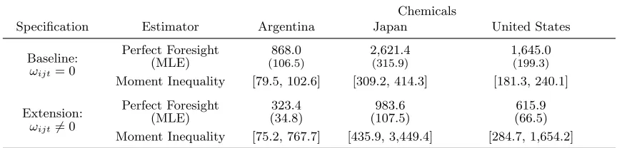
Table 3: Average fixed export costs

Chemicals Food

Estimator Argentina Japan United States Argentina Japan United States

Perfect Foresight 868.0 2,621.4 1,645.0 2,049.3 2,395.1 2,202.5

(MLE) (150.1) (468.2) (290.7) (213.8) (259.4) (233.8)

Minimal Information 348.7 1,069.4 668.1 1,273.9 1,482.4 1,366.3

(MLE) (49.9) (142.2) (90) (221.8) (272.9) (244.2)

Moment Inequality [79.5, 102.6] [309.2, 414.3] [181.3, 240.1] [175.6, 270.1] [269.1, 361.0] [227.3, 308.9]

Notes: All estimates are reported in thousands of year 2000 USD and their values scale proportionally withη, which is set equal to 5 (see Section 2.4). For the two ML estimators, bootstrap standard errors are computed according to the procedure described in Appendix A.6 and reported in parentheses. For the three moment inequality estimates, extreme points of the 95% confidence set are reported in square brackets. These confidence sets are projections of a confidence set for (β0, β1, σ) computed according to the procedure described in Appendix A.7.

Table 4: Average fixed export costs relative to perfect foresight estimates

Chemicals Food

Estimator Argentina Japan United States Argentina Japan United States

Minimal Info. 40.2% 40.8% 40.6% 62.2% 61.9% 62.0%

Moment Ineq. [9.1%, 11.9%] [11.8%, 15.8%] [11.1%, 14.6%] [8.6%, 1