Studies in Income and Wealth Volume 77
Education, Skills, and
Technical Change
Implications for Future
US GDP Growth
Edited by
Charles R. Hulten
and Valerie A. Ramey
The University of Chicago Press
The University of Chicago Press, Chicago 60637 The University of Chicago Press, Ltd., London © 2019 by the National Bureau of Economic Research
All rights reserved. No part of this book may be used or reproduced in any manner whatsoever without written permission, except in the case of brief quotations in critical articles and reviews. For more information, contact the University of Chicago Press, 1427 E. 60th St., Chicago, IL 60637.
Published 2019
Printed in the United States of America
28 27 26 25 24 23 22 21 20 19 1 2 3 4 5
ISBN- 13: 978- 0- 226- 56780- 8 (cloth) ISBN- 13: 978- 0- 226- 56794- 5 (e- book)
DOI: https:// doi .org /10 .7208 /chicago /9780226567945 .001 .0001
Library of Congress Cataloging- in- Publication Data
Names: Education, Skills, and Technical Change: Implications for Future U.S. GDP Growth (Conference) (2015 : Bethesda, Maryland) | Hulten, Charles R., editor. | Ramey, Valerie A. (Valerie Ann), editor.
Title: Education, skills, and technical change : implications for future US GDP growth / edited by Charles R. Hulten and Valerie A. Ramey.
Other titles: Studies in income and wealth ; v. 77.
Description: Chicago : The University of Chicago Press, 2019. | Series: Studies in income and wealth ; v. 77 | “This volume contains revised versions of the papers presented at the Conference on Research in Income and Wealth titled “Education, Skills, and Technical Change: Implications for Future U.S. GDP Growth,” held in Bethesda, Maryland, on October 16–17, 2015”—Publisher info. | Includes bibliographical references and index.
Identifi ers: LCCN 2018013221 | ISBN 9780226567808 (cloth : alk. paper) | ISBN 9780226567945 (e- book)
Subjects: LCSH: Labor supply—Eff ect of education on—United States—Congresses. | Labor supply—Eff ect of technological innovations on—United States—Congresses. | Education—Eff ect of technological innovations on—United States—Congresses. | Gross domestic product—Social aspects—United States—Congresses. | Human capital—United States—Congresses.
Classifi cation: LCC HD5724 .E28 2019 | DDC 338.973—dc23 LC record available at https:// lccn .loc .gov /2018013221
♾ This paper meets the requirements of ANSI/NISO Z39.48- 1992 (Permanence of Paper).
National Bureau of Economic Research
Offi cers
Karen N. Horn, chair John Lipsky, vice chair
James M. Poterba, president and chief executive offi cer
Robert Mednick, treasurer
Kelly Horak, controller and assistant corporate secretary
Alterra Milone, corporate secretary Denis Healy, assistant corporate secretary
Directors at Large
Peter C. Aldrich Elizabeth E. Bailey John H. Biggs John S. Clarkeson Kathleen B. Cooper Charles H. Dallara George C. Eads Jessica P. Einhorn
Mohamed El- Erian Jacob A. Frenkel Robert S. Hamada Peter Blair Henry Karen N. Horn Lisa Jordan John Lipsky Laurence H. Meyer Karen Mills Michael H. Moskow Alicia H. Munnell Robert T. Parry James M. Poterba John S. Reed Marina v. N. Whitman Martin B. Zimmerman
Directors by University Appointment
Timothy Bresnahan, Stanford Pierre- André Chiappori, Columbia Alan V. Deardorff , Michigan Ray C. Fair, Yale
Edward Foster, Minnesota John P. Gould, Chicago
Mark Grinblatt, California, Los Angeles Bruce Hansen, Wisconsin–Madison Benjamin Hermalin, California, Berkeley
George Mailath, Pennsylvania Marjorie B. McElroy, Duke Joel Mokyr, Northwestern Cecilia Rouse, Princeton
Richard L. Schmalensee, Massachusetts Institute of Technology
Ingo Walter, New York David B. Yoffi e, Harvard
Directors by Appointment of Other Organizations
Jean- Paul Chavas, Agricultural and Applied Economics Association
Martin J. Gruber, American Finance Association
Philip Hoff man, Economic History Association
Arthur Kennickell, American Statistical Association
Jack Kleinhenz, National Association for Business Economics
Robert Mednick, American Institute of Certifi ed Public Accountants Peter L. Rousseau, American Economic
Association
Gregor W. Smith, Canadian Economics Association
William Spriggs, American Federation of Labor and Congress of Industrial Organizations
Bart van Ark, The Conference Board
Relation of the Directors to the Work and Publications of the
National Bureau of Economic Research
1. The object of the NBER is to ascertain and present to the economics profession, and to the public more generally, important economic facts and their interpretation in a scientifi c manner without policy recommendations. The Board of Directors is charged with the responsibility of ensuring that the work of the NBER is carried on in strict conformity with this object.
2. The President shall establish an internal review process to ensure that book manuscripts pro-posed for publication DO NOT contain policy recommendations. This shall apply both to the proceedings of conferences and to manuscripts by a single author or by one or more co- authors but shall not apply to authors of comments at NBER conferences who are not NBER affi liates. 3. No book manuscript reporting research shall be published by the NBER until the President has sent to each member of the Board a notice that a manuscript is recommended for publica-tion and that in the President’s opinion it is suitable for publicapublica-tion in accordance with the above principles of the NBER. Such notifi cation will include a table of contents and an abstract or summary of the manuscript’s content, a list of contributors if applicable, and a response form for use by Directors who desire a copy of the manuscript for review. Each manuscript shall contain a summary drawing attention to the nature and treatment of the problem studied and the main conclusions reached.
4. No volume shall be published until forty- fi ve days have elapsed from the above notifi cation of intention to publish it. During this period a copy shall be sent to any Director requesting it, and if any Director objects to publication on the grounds that the manuscript contains policy recommendations, the objection will be presented to the author(s) or editor(s). In case of dispute, all members of the Board shall be notifi ed, and the President shall appoint an ad hoc committee of the Board to decide the matter; thirty days additional shall be granted for this purpose.
5. The President shall present annually to the Board a report describing the internal manu-script review process, any objections made by Directors before publication or by anyone after publication, any disputes about such matters, and how they were handled.
6. Publications of the NBER issued for informational purposes concerning the work of the Bureau, or issued to inform the public of the activities at the Bureau, including but not limited to the NBER Digest and Reporter, shall be consistent with the object stated in paragraph 1. They shall contain a specifi c disclaimer noting that they have not passed through the review procedures required in this resolution. The Executive Committee of the Board is charged with the review of all such publications from time to time.
7. NBER working papers and manuscripts distributed on the Bureau’s web site are not deemed to be publications for the purpose of this resolution, but they shall be consistent with the object stated in paragraph 1. Working papers shall contain a specifi c disclaimer noting that they have not passed through the review procedures required in this resolution. The NBER’s web site shall contain a similar disclaimer. The President shall establish an internal review process to ensure that the working papers and the web site do not contain policy recommendations, and shall report annually to the Board on this process and any concerns raised in connection with it.
vii
Prefatory Note ix
Introduction 1
Charles R. Hulten and Valerie A. Ramey
I. The Macroeconomic Link between Education and Real GDP Growth
1. Educational Attainment and the Revival of US
Economic Growth 23 Dale W. Jorgenson, Mun S. Ho,
and Jon D. Samuels
2. The Outlook for US Labor- Quality Growth 61 Canyon Bosler, Mary C. Daly, John G. Fernald, and Bart Hobijn
Comment on Chapters 1 and 2:
Douglas W. Elmendorf
3. The Importance of Education and Skill Development for Economic Growth in the
Information Era 115 Charles R. Hulten
II. Jobs and Skills Requirements
5. The Requirements of Jobs: Evidence from a
Nationally Representative Survey 183 Maury Gittleman, Kristen Monaco,
and Nicole Nestoriak
III. Skills, Inequality, and Polarization
6. Noncognitive Skills as Human Capital 219 Shelly Lundberg
Comment: David J. Deming
7. Wage Inequality and Cognitive Skills:
Reopening the Debate 251 Stijn Broecke, Glenda Quintini,
and Marieke Vandeweyer
Comment: Frank Levy
8. Education and the Growth- Equity Trade- Off 293 Eric A. Hanushek
9. Recent Flattening in the Higher Education Wage Premium: Polarization, Skill
Downgrading, or Both? 313 Robert G. Valletta
Comment: David Autor
IV. The Supply of Skills
10. Accounting for the Rise in College Tuition 357 Grey Gordon and Aaron Hedlund
Comment: Sandy Baum
11. Online Postsecondary Education and
Labor Productivity 401 Caroline M. Hoxby
Comment: Nora Gordon
12. High- Skilled Immigration and the Rise of
STEM Occupations in US Employment 465 Gordon H. Hanson and Matthew J. Slaughter
Comment: John Bound
Contributors 501
Author Index 505
ix This volume contains revised versions of the papers presented at the Confer-ence on Research in Income and Wealth titled “Education, Skills, and Tech-nical Change: Implications for Future U.S. GDP Growth,” held in Bethesda, Maryland, on October 16–17, 2015.
We gratefully acknowledge the fi nancial support for this conference pro-vided by the Bureau of Economic Analysis. Support for the general activities of the Conference on Research in Income and Wealth is provided by the fol-lowing agencies: Bureau of Economic Analysis, Bureau of Labor Statistics, Bureau of the Census, Board of Governors of the Federal Reserve System, Statistics of Income/Internal Revenue Service, and Statistics Canada.
We thank Charles R. Hulten and Valerie A. Ramey, who served as confer-ence organizers and as editors of the volume.
Executive Committee, December 2016
John M. Abowd Barry Johnson
Katharine Abraham (chair) André Loranger
Susanto Basu Brian Moyer
Andrew Bernard Valerie A. Ramey
Ernst R. Berndt Mark J. Roberts
Carol A. Corrado Peter Schott
357 10.1 Introduction
Over the past thirty years, the perceived necessity of a college degree and a growing college earnings premium have led to record enrollments and greater degree attainment in higher education. However, a dramatic escala-tion in tuiescala-tion looms over the heads of prospective students and their parents and serves as a stark reminder to graduates saddled with large student loans. From 1987 to 2010, sticker price tuition and fees ballooned from $6,630 to $14,510 in 2010 dollars. After subtracting institutional aid, net tuition and fees still grew by 92 percent, from $5,720 to $11,000. To provide perspective, had net tuition risen at the rate of much maligned health care costs, tuition would have only risen 32 percent to $7,550 in 2010.1
In this chapter, we seek to account for the college tuition increase by quan-titatively evaluating existing explanations using a structural model of higher education and the macroeconomy. We divide our hypotheses about driv-ing forces into supply- side changes (Baumol’s cost disease and exogenous
1. Calculations used the health care personal consumption expenditures price index defl ated by the CPI.
Accounting for the Rise in
College Tuition
Grey Gordon and Aaron Hedlund
Grey Gordon is assistant professor of economics at Indiana University. Aaron Hedlund is assistant professor of economics at the University of Missouri.
changes to nontuition revenue), demand- side changes (notably, expansions in grant aid and loans), and macroeconomic forces (namely, skill- biased technical change resulting in a higher college earnings premium). Our quan-titative model shows that the combined eff ect of these changes more than accounts for the tuition increase and provides key insights about the role of individual factors as well as their complementary eff ects.
Existing hypotheses of why college tuition is increasing largely fall into two camps: those that emphasize the unique virtues and pathologies of higher education and those that place rising higher education costs into a broader narrative of increasing prices in many service industries. Advocates of the latter approach look to cost disease and skill- biased technical progress as drivers of higher costs in service industries that employ highly skilled labor. Cost disease, which dates back to seminal papers by Baumol and Bowen (1966) and Baumol (1967), posits that economy- wide productivity growth pushes up wages and creates cost pressures on service industries that do not share in the productivity growth. To cope, these industries increase their relative price, passing their higher costs onto consumers.
By contrast, theories emphasizing the uniqueness of higher education take several forms. Falling within our notion of supply- side shocks, state and local funding for higher education fell from $8,200 per full- time equivalent (FTE) student in 1987 to $7,300 in 2010, all while underlying costs and expenditures were rising. Several studies, including a notable study com-missioned by Congress in the 1998 reauthorization of the Higher Education Act, attribute a sizable fraction of the increase in public university tuition to these state funding cuts. We take a somewhat broader view in this chapter by looking at how exogenous changes to all sources of nontuition revenue impact the path of tuition.
On the demand side, several expansions in fi nancial aid have occurred over the past several decades. During our period of analysis, annual and aggre-gate subsidized Staff ord loan limits were increased in 1987 and fi ve years later in 1992. The Higher Education Amendments of 1992 also established a program of supplementary unsubsidized Staff ord loans and increased the annual PLUS loan limit to the cost of attendance minus aid, thereby elimi-nating aggregate PLUS loan limits. Interest rates on student loans also fell considerably during the fi rst decade of the twenty- fi rst century. In a famous 1987 New York Times op- ed titled “Our Greedy Colleges,” then- secretary of education William Bennett asserted that “increases in fi nancial aid in recent years have enabled colleges and universities blithely to raise their tuitions” (Bennett 1987). We evaluate this claim through the lens of our model, and we also cast light on the tuition impact of the 53 percent rise in nontuition costs (such as those arising from the greater provision of student amenities), which has the eff ect of increasing subsidized loan eligibility.
Kearney (2008) fi nd that, from the mid- 1980s to 2005, the overall earn-ings premium for having a college degree increased from 58 percent to over 93 percent. Ceteris paribus, such an increase in the return to college has assuredly driven up demand for a college degree. We use our model to quan-tify how much this increase in demand translates to higher tuition and how much it contributes to higher enrollments.
Our quantitative fi ndings can be summarized as follows:
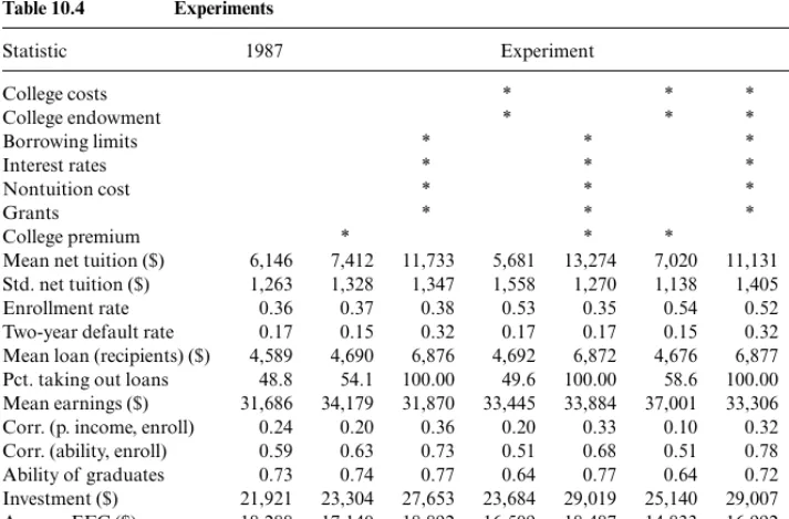
1. The combined eff ect of the aforementioned shocks generates a 102 percent increase in equilibrium tuition. This result compares to a 92 percent increase in the data.
2. The rise in the college earnings premium alone causes tuition to increase by 21 percent. With all other shocks present except the college premium hike, tuition increases by 81 percent.
3. The demand- side shocks by themselves cause tuition to jump by 91 per-cent. With all other changes except the demand- side shocks, tuition only increases by 14 percent.
4. The supply- side shocks by themselves cause tuition to decline by 8 per-cent. With all other changes except the supply- side shocks, tuition increases by 116 percent.
The model we construct to arrive at these conclusions embeds a rich higher education framework based off of Epple, Romano, and Sieg (2006) and Epple et al. (2013) into a life- cycle environment with heterogeneous agents, incomplete markets, and student loan default. Imperfectly competi-tive colleges in the model set diff erential tuition and admissions policies to maximize quality, which, as a proxy for reputation, depends on investment per student and the average academic ability of the heterogeneous student body. In this chapter, we restrict attention to the case of a representative nonprofi t institution that has limited market power because of unobservable student preference shocks. Even with these shocks, the representative col-lege assumption still abstracts from important heterogeneity and strategic interactions in the higher education market. For this reason, the fi ndings in this chapter should be used to guide further research rather than viewed authoritatively. To further simplify matters, we treat all nontuition revenue as exogenous (e.g., endowment income and state funding), which implies that the college faces a balanced budget constraint each period that equates total revenue with total spending on investment and non- quality- enhancing custodial costs. On the household side, we include several important features: heterogeneity in ability and parental income dimensions, college fi nancing decisions, college dropout risk, and student loan repayment decisions.
The objective of selective academic institutions is to be the best they can in every aspect of their activities. They aggressively seek out all possible resources and put them to use funding things they think will make them better. To look better than their competitors, the institutions wind up in an arms race of spending.
To make matters concrete, quality in our setting depends on investment per student and the average ability of the student body. As a result, students act both as customers and as inputs to the production of quality via peer eff ects, as described by Winston (1999). This unique feature of higher edu-cation gives colleges an additional motive to engage in price discrimination beyond the usual monetary rent extraction—namely, to attract high- ability students by off ering generous institutional aid.
To discipline the model, we use a combination of calibration and esti-mation. Rather than ex ante assume cost disease or a particular produc-tion structure (e.g., number of faculty, administrators, etc., needed to run a college), we directly estimate a reduced- form custodial cost function and track its changes over the period 1987–2010. Similarly, we compute average nontuition revenue per FTE student using Delta Cost Project data and feed it into the model. On the household side, we use earnings premium estimates by Autor, Katz, and Kearney (2008) and construct time series for federal student loan program (FSLP) variables.
As mentioned previously, we fi nd that the combined eff ects of the supply- side changes, demand- side changes, and increases in the college earnings premium can fully account for the mean net tuition increase. Looking at individual factors, we fi nd that expansions in borrowing limits drive 54 per-cent of the tuition jump and represent the single most important factor.2 To grasp the magnitude of the change in borrowing capacity, fi rst note that real aggregate borrowing limits increased by 56 percent between 1987 and 2010, from $26,200 to $40,800 in 2010 dollars.3 Second, the reauthorization of the Higher Education Act in 1992 introduced a major change along the extensive margin by establishing an unsubsidized loan program alongside the subsidized loans. We also fi nd that increased grant aid contributes 18 percent to the rise in tuition, which mirrors the 21 percent impact of the higher college earnings premium. These results give credence to the Bennett (1987) hypothesis.
Last, our results, while preliminary and subject to the caveat mentioned above regarding the representative college assumption, paint a more nuanced picture of cost disease as a driver of higher tuition. Although our estimated cost function shifts upward from 1987 to 2010, this isolated eff ect reduces
2. For this calculation, we take one minus the tuition increase without the borrowing limit expansion relative to the increase with the expansion, that is, 1 − ($9,066 − $6,146)/($12,428 − $6,146). Adding the percentage contribution from each exogenous driving force need not yield 100 percent because of interaction eff ects.
average tuition (a contribution of −16 percent). Importantly, our estimates suggest that the upward shift in the cost function between 1987 and 2010 comes largely in the form of higher fi xed costs rather than higher marginal costs, which has important implications for how colleges respond. Intui-tively, colleges face a trade- off between raising tuition and retaining high- ability students when they experience a balance sheet deterioration. If they increase tuition, fewer high- ability students may enroll, which drives down quality. Alternatively, a decision to not raise tuition forces colleges to cut back on quality- enhancing investment expenditures. We fi nd that colleges take this latter route to the tune of almost $2,800 in cuts per student as a response to higher custodial costs. This result comports with the behavior we observe among many public universities across the country of replacing tenured faculty with less expensive non- tenure- track positions. Additionally, changes in nontuition revenue have almost no impact on tuition (a contribu-tion of 2 percent).
We do not claim that Baumol’s cost disease or changes in state support have no importance for tuition increases. Rather, we suspect that these fac-tors aff ect some colleges more than others. For instance, if private research universities experience cost disease, they may increase their tuition. How-ever, higher tuition may induce substitution of students into lower- cost uni-versities. Given the absence of competition and college heterogeneity in our model, our estimation implicitly incorporates substitution of households across college types and any corresponding composition eff ects.
10.1.1 Relationship to the Literature
This chapter relates to two broad strands of the literature. First, the chapter relates to a large empirical literature that estimates the eff ects of macroeconomic factors and policy interventions on tuition and enrollment. Second, this chapter relates to a growing body of literature employing struc-tural models of higher education. With a few exceptions, these models focus on student demand and abstract from many distinguishing features of the supply side.
Empirical Literature
In discussing related work, we map our categorization of supply- side shocks, demand- side shocks, and macroeconomic forces into the exist-ing empirical literature. For supply- side shocks, we analyze the impact of upward shifts in custodial (non- quality- enhancing) costs as well as changes in nontuition revenues. The literature on Baumol’s cost disease most closely relates to the former, while the literature analyzing the eff ect of the decline in state appropriations for higher education addresses the latter.
up wages everywhere, which service sectors that lack productivity growth pass along by increasing their relative prices. Recently, Archibald and Feld-man (2008) use cross- sectional industry data to forcefully advance the idea that cost and price increases in higher education closely mirror trends for other service industries that utilize highly educated labor. In short, they “reject the hypothesis that higher education costs follow an idiosyncratic path.”
We fi nd that the form of the cost increase matters. In particular, our esti-mates uncover a large increase in the fi xed cost of operating a college from $12 billion to $30 billion in 2010 dollars. To pay for the higher fi xed cost, the college in our model lowers per- student investment and increases enroll-ment, which lowers average tuition by a composition eff ect.
Supply Shocks: Cuts in State Appropriations. Heller (1999) suggests a negative relationship between state appropriations for higher education and tuition, asserting that “the higher the support provided by the state, the lower generally is the tuition paid by all students.” Recent empirical work by Chakrabarty, Mabutas, and Zafar (2012), Koshal and Koshal (2000), and Titus, Simone, and Gupta (2010) support this hypothesis, but notably, Titus, Simone, and Gupta (2010) show that this relationship only holds up in the short run. Last, in a large study commissioned by Congress in the 1998 reauthorization of the Higher Education Act of 1965, Cunningham et al. (2001) conclude that “Decreasing revenue from government appropriations was the most important factor associated with tuition increases at public four- year institutions.”
While our model fails to confi rm this idea in the aggregate—that is, lumping public and private colleges together—cuts in appropriations could potentially play a role in driving up public school tuition. Extending our model to incorporate heterogeneous colleges with detailed, disaggregated funding data will shed further light on this issue.
Demand Shocks: The Bennett Hypothesis. For demand- side shocks, we focus on the eff ects of increased fi nancial aid. We address the extent to which changes in loan limits and interest rates under the FSLP as well as expan-sions in state and federal grants to students drive up tuition—famously known as the Bennett hypothesis. A long line of empirical research has studied this hypothesis with mixed results.
339) come to the mirror opposite conclusion: “We fi nd substantial evidence that increases in the generosity of the federal Pell Grant program, access to subsidized loans, and state need- based grant aid awards lead to increases in in- state tuition levels. However, we fi nd no evidence that nonresident tuition is increased as a result of these programs.” Turner (2012) shows that tax- based aid crowds out institutional aid almost one- for- one. Turner (2014) also fi nds that institutions capture some of the benefi ts of fi nancial aid, but at a more modest 12 percent pass- through rate. Long (2004a, 2004b) uncovers evidence that institutions respond to greater aid by increasing charges, in some cases by up to 30 percent of the aid. Cellini and Goldin (2014) compare for- profi t institutions that participate in federal student aid programs to those that do not participate. Institutions in the former group charge tuition that is about 78 percent higher than those in the latter group. Most recently, Lucca, Nadauld, and Shen (2015) fi nd a 65 percent pass- through eff ect for changes in federal subsidized loans and positive but smaller pass- through eff ects for changes in Pell grants and unsubsidized loans.
In contrast to the previous literature, several papers reject or fi nd little evidence for the Bennett hypothesis. For example, in their commissioned report for the 1998 reauthorization of the Higher Education Act, Cunning-ham et al. (2001, x) conclude that “the models found no associations between most of the aid variables and changes in tuition in either the public or private not- for- profi t sectors.” These sentiments are echoed by Long (2006). Last, Frederick, Schmidt, and Davis (2012) study the response of community col-leges to changes in federal aid and fi nd little evidence of capture.
Our model likely exaggerates the impact of the Bennett hypothesis. As we discuss in section 10.4, the representative college engages in an implausibly high degree of rent extraction despite the presence of preference shocks. We suspect that more competition in our model of the higher education market would temper the magnitude of the tuition increase attributable to the Bennett hypothesis.
Macroeconomic Forces: Rising College Earnings Premiums. According to data from Autor, Katz, and Kearney (2008), the college earnings pre-mium increased from 58 percent in the mid- 1980s to 93 percent in 2005. While we remain agnostic about the cause of the increasing premium, sev-eral papers, including Autor, Katz, and Kearney (2008), Katz and Murphy (1992), Goldin and Katz (2007), and Card and Lemieux (2001), ascribe it to skill- biased technological change combined with a fall in the relative supply of college graduates.
else-where. Incorporating this heterogeneity in college earnings premiums may help explain why tuition increases at selective schools (such as public and private research universities) have outpaced those at less selective schools.
Quantitative Models of Higher Education
Our chapter also fi ts into a growing body of papers that employ structural models of higher education such as Abbott et al. (2013), Athreya and Eberly (2013), Ionescu and Simpson (2016), Ionescu (2011), Garriga and Keightley (2010), Lochner and Monge- Naranjo (2011), Belley and Lochner (2007), and Keane and Wolpin (2001). In the interest of space, we discuss only the most closely related papers.
Recent work by Jones and Yang (2016) closely mirrors the objectives of this chapter. They explore the role of skill- biased technical change in explaining the rise in college costs from 1961 to 2009. Their paper diff ers from our chapter in several ways. First, whereas they explore the eff ect of cost disease on higher college costs, we quantify the role of supply- side as well as demand- side shocks. Second, Jones and Yang (2016) analyze college costs—which increased by 35 percent in real terms between 1987 and 2010— whereas we address the increase in net tuition, which went up by 92 percent. Also, whereas they use a competitive framework, we employ a model with peer eff ects, imperfect competition with price discrimination, and student loan borrowing with default. Fillmore (2014) also analyzes a model of price discriminating colleges, but he treats peer eff ects in a reduced- form way. Fu (2014) considers a rich game- theoretic framework of college admissions and enrollment but does not allow for price discrimination.
10.2 The Model
The model embeds a college sector into a discrete- time open economy. A fi xed measure of heterogeneous households enter the economy upon gradu-ating high school, make college enrollment decisions, and then progress through their working life and into retirement. A monopolistic college with the ability to price discriminate transforms students into college graduates (with dropout risk), and the government levies taxes to fi nance student loans.
10.2.1 Households
We describe sequentially the environment faced by youths, college stu-dents, and fi nally, workers and retirees. We immediately follow this discus-sion with a description of colleges in the model. Section 10.2.4 gives the decision problems for all agents in the economy.
Youths
of characteristics sY = (x, yp) consisting of academic ability x and parental income yp from a distribution G. Youths make a once- and- for- all choice to either enroll in college or enter the workforce. In addition to the explicit pecuniary and nonpecuniary benefi ts of college that we will describe momentarily, youths receive a preference shock (1/α)ε of attending college, where α > 0 and ε comes from a type 1 extreme distribution. Colleges cannot condition tuition on the preference shock.
College Students
Newly enrolled students enter college with their vector of characteristics
sY and a zero initial student loan balance, l = 0. Colleges charge type- specifi c net tuition T (sY)—equal to sticker price T minus institutional aid—which they hold fi xed for the duration of enrollment.
Students also face nontuition expenses ϕ that act as perfect substitutes for consumption c. Direct government grants ζ(T + ϕ, EFC(sY)) off set some of the cost of attendance, where EFC(sY) represents the expected family contribution—a formula used by the government to determine eligibility for need- based grants and loans. After taking into account both forms of aid, the net cost of attendance comes out to NCOA(sY) = T (sY) + ϕ – ζ(T (sY) + ϕ, EFC(sY)).
While enrolled, college students receive additively separable fl ow utility
v (q), which increases in college quality q.4 In order to graduate, students must complete JY years of college. Students in class j return to college each year with probability j+1 1[j+1JY]; otherwise, they either drop out or
grad-uate.5
Students can borrow through the FSLP. Of primary interest, the FSLP features subsidized loans that do not accrue interest while the student is in college, where eligibility depends on fi nancial need (NCOA less EFC). Since 1993, students can borrow additional funds up to the net cost of attendance using unsubsidized loans. Students face annual and aggregate limits for sub-sidized and combined borrowing.
Denote the annual and aggregate combined limits by bj and l, respec-tively.6 Because students can borrow only up to the net cost of attendance, their annual combined subsidized borrowing bs and unsubsidized borrowing
bu must satisfy
(1) bs+bu min{bj, NCOA(sY)}.
4. To improve tractability while computing the transition path, we assume students receive v (q) each year based on the college’s quality q at the time of initial enrollment. In the computa-tion, we make the isomorphic assumption that students receive the net present value of v (q) at the time of enrollment.
5. We do not allow endogenous dropout for reasons of tractability.
Similarly, defi ne bjs as the statutory annual subsidized limit and l
js as the
statutory aggregate subsidized limit. The actual amount bjs s Y
( ) that students can borrow in subsidized loans depends on their net cost of attendance and the expected family contribution, both of which vary with student type. Last, defi ne ljs s
Y
( ) as the maximum amount of subsidized loans that students can accumulate by year j in college. Mathematically,
(2) bjs(s
Y) = min{bjs, max{0, NCOA(sY) EFC(sY)}} ljs(sY) = min{ls, ij=1bis(sY)}.
Given the superior fi nancial terms of subsidized loans, we assume that stu-dents always exhaust their subsidized borrowing capacity before taking out any unsubsidized loans. Furthermore, to increase tractability, we assume that borrowers can carry over unused subsidized borrowing capacity into subsequent years. These two assumptions reduce the state space and signifi -cantly simplify the student’s debt portfolio choice problem.
Apart from loans, students have two other means of paying for college. First, they have earnings eY, which we treat as an endowment.7 Second, they receive a parental transfer ξEFC(sY), where 0 ≤ ξ ≤ 1 is a parameter.
Workers/Retirees
Working and retired households receive earnings e that depend on a vec-tor of characteristics s that includes their level of education, age/retirement status, and a stochastic component. Each period, households face a propor-tional earnings tax τ.
These households value consumption according to a period utility func-tion u(c) and discount the future at rate β. Workers with student loans face a loan interest rate of i and amortization payments of p(l, t ) = l{[i (1 + i)t–1] /
[(1 + i )t – 1]} where l represents the loan balance and t the remaining
dura-tion. All households can use a discount bond to save at the risk- free rate
r* and borrow up to the natural borrowing limit a at rate r* + ι, where ι is the interest premium on borrowing. The price of the bond is denoted (1 +
r (a′))–1.
10.2.2 Colleges
There is one representative college. Following Epple, Romano, and Sieg (2006), the college seeks to maximize its quality (or prestige), q, which depends on the average academic ability θ of the student body and on investment expenditures per student, I. The college’s other expenses include non- quality- enhancing custodial costs F +C({Nj}JjY=1), where F represents a
fi xed cost and C is an increasing, twice- diff erentiable, convex function of enrollment {Nj}JjY=1.
The college fi nances its expenditures with two sources of revenue. First, the college has exogenous nontuition revenue per student E, which includes endowment income, government appropriations, and revenues from aux-iliary enterprises. Second, the college has endogenous tuition revenue, a function of enrollment decisions and type- specifi c net tuition T (sY). The college is a nonprofi t and, given our assumption of an exogenous endow-ment stream, runs a balanced budget period- by- period.8
In order to avoid dealing with issues such as the college’s discount fac-tor—not to mention other diffi culties associated with the transition path computation—we make the college problem static through four assump-tions. First, we assume that college quality q (θ, I ) depends on the academic ability of freshmen and investment expenditures per freshman student.9 Sec-ond, we assume that colleges face a quadratic cost function for each class given by
(3) F +C({Nj}Jj=Y1) = F + j=1 JY
c(nj)
where Nj is the population measure in class j ( j = 1 for freshmen, j = 2 for sophomores, etc.) and nj≡ Nj/ (1/J ) is the measure relative to the age- eighteen population (for scaling purposes in the estimation). Third, we assume the college has no access to credit markets. Last, we isolate the eff ect of current tuition and spending decisions on future budget conditions. Specifi cally, we assume that each year the college exchanges the rights to all future budget fl ows generated by contemporaneous tuition and expenditure decisions in exchange for an immediate net present value payment from the government. This last assumption implicitly rules out any “quality smoothing” on the part of the college and captures the fact that administrators typically have short tenures that may make borrowing against expected future fl ows challenging.10
10.2.3 Legal Environment and Government Policy
Consistent with US law, workers in the model cannot liquidate their stu-dent loan debt through bankruptcy. However, they can skip payments and become delinquent. Upon initial default, workers enter delinquency status and face a proportional loan penalty of η that accrues to their existing bal-ance. In subsequent periods, delinquent workers face a proportional wage garnishment of γ until they rehabilitate their loan by making a payment. Upon rehabilitation, the loan duration resets to the statutory value tmax and the amortization schedule adjusts accordingly.
The government operates the student loan program and fi nances itself
8. Technically, the nonprofi t status of the college only implies that it cannot distribute divi-dends. However, we abstract from strategic decisions regarding endowment accumulation.
9. We assume the college commits to a level of I for the duration of each incoming cohort’s enrollment.
with a combination of taxation on labor earnings, funds from loan repay-ments and wage garnishrepay-ments, and the revenue fl ows generated by colleges discussed above. We assume that the government sets the tax rate τ to bal-ance its budget period- by- period.
10.2.4 Decision Problems
Now we work backward through the life cycle to describe the household- decision problem. Afterward, we describe the college’s optimization prob-lem.
Workers/Retirees
Households start each period with asset position a, student loan balance
l and duration t, characteristics s, and delinquency status f {0,1}, where
f = 0 indicates good standing. Households in good standing on their student
loans choose consumption, savings, and whether to make their scheduled loan payment. These households have the value function
(4) V(a,l,t,s,f =0) = max{VR(a,l,t,s),VD(a,l(1+ ),s)}
where VR is the utility of repayment and VD is the utility of delinquency.
Note that η increases the stock of outstanding debt in the case of a default. Households in bad standing face the decision of whether to rehabilitate their loan or remain delinquent. Their value function is
(5) V(a,l,s,f =1)= max{VR(a,l,t
max,s),VD(a,l,s)}.
Household utility conditional on repayment or rehabilitation is given by
(6) VR(a,l,t,s)= max
c 0,a au(c)+ s|sV(a,l,t,s,f =0)
subject to
c+a/(1+r(a))+ p(l,t) e(s)(1 )+a l = (l p(l,t))(1+i),t = max{t 1,0}.
The value of defaulting (if f = 0) or not rehabilitating a loan (if f = 1) is11
(7) VD(a,l,s) = max
c 0,a au(c)+ s|sV(a,l,s,f =1)
subject to
c+a/(1+r(a)) e(s)(1 )(1 )+a l = max{0,(l e(s)(1 ) )(1+i)}.
In the last period of life, households have no continuation utility and no ability to borrow or save. We allow households to die with student loan debt.
College Students
College students with characteristics sY = (x, yp) and debt l choose con-sumption and additional loans, l′ ≥ l (to speed up computation, we assume that students do not pay back their loans while in college). We also introduce an annual unsubsidized borrowing limit bju that equals either the combined
limit or zero (the latter case captures the pre- 1993 environment).
Taking college quality q and the net tuition function T() as given, stu-dents solve
(8) Yj(l,sY;T,q) = max
c 0,l lu(c+ )+v(q)+
j+1Yj+1(l,sY;T)+(1 j+1) s|j,sYV(a =0,l,tmax,s,0)
subject to
c+NCOA(sY) eY + EFC(sY)+bs+bu
(ls,lu)=
(l,0) if l ljs(sY)
(ljs(sY),l ljs(sY)) otherwise
(ls,lu)=
(l,0) if l ljs1(sY)
(ljs1(sY),l ljs1(sY)) otherwise
bs =ls ls bu = lu
1+i =lu l + lu
1+i l
bu min{bju, NCOA(sY)}
bs+bu min{bj, NCOA(sY)}.
Note from these equations that our setup allows us to easily decompose student debt into its subsidized and unsubsidized components. We defl ate
lu by 1 + i in the aggregate borrowing constraint because the loan limit is inclusive of interest accrued by unsubsidized loans.
Youth
Youth making their college enrollment decisions have value function
(9) max s|sYV1(a =0,l = 0,t =0,s)
enterthelaborforce
,Y1(l = 0,sY;T,q)+
1
where denotes the college preference shock and s is the initial worker char-acteristics draw.
Colleges
The college problem can be written as
(10) max
I 0,T( )q( ,I)
subject to
E+T = F+C(N1)+J
N1= (enroll|sY;T( ),q)d 0(sY) N1= x(sY) (enroll|sY;T( ),q)d 0(sY)
T = j=1
JY
j 1 T(s
Y) (enroll|sY;T( ),q)d 0(sY)
(1+r*)j 1
E = E j=1
JY
j 1N
1
(1+r*)j 1
C(N1)= JjY=1
c{ j 1[N 1/(1/J)]}
(1+r*)j 1
J = I JjY=1
j 1N
1
(1+r*)j 1
where 0( )sY G s( )Y /J is the distribution of characteristics across the age-
eighteen population.
The fi rst constraint refl ects the college balanced budget requirement, while the remaining constraints establish the defi nitions of enrollment, aver-age freshman ability, tuition revenues, nontuition revenues, custodial costs, and investment expenditures, respectively.
10.2.5 Steady- State Equilibrium
A steady- state equilibrium consists of household value and policy func-tions, a tax rate, college policies and quality, and a distribution of house-holds such that
1. The household value and policy functions satisfy (4–9). 2. The college policies and quality satisfy (10).
10.3 Data and Estimation
We calibrate the model to replicate key features of the US economy and higher education sector in 1987. These initial conditions set the stage for the results section, which feeds in the observed changes between 1987 and 2010 described in the introduction to assess their impact on equilibrium tuition. We proceed through our description of the calibration and estimation in the same order as we described the model.
10.3.1 Households
Youths
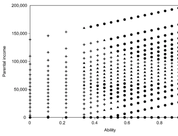
We determine the distribution G of youth characteristics sY = (x, yp) using data from the National Longitudinal Survey of Youth 1997 (NLSY97). The ability measure comes from percentiles on the Armed Services Vocational
Aptitude Battery (ASVAB) test. For parental income, we use the household
income measure from 1997 in those cases where the data correspond to the parents rather than the youth (98.0 percent of cases).
Conditional on our ability measure, parental income resembles a trun-cated normal distribution. This can be seen in fi gure 1 of web appendix A (http:// www .nber .org /data - appendix /c13711 /appendix .pdf). To handle truncation from above due to top- coding and truncation from below, we estimate a Tobit model where parental income depends on ability. Specifi -cally, we estimate
(11) yi*= 0+ 1xi+ i yi = min{max{0,yi*},y}
where yi is the observed parental income, yi* is the “true” parental income, and i ~ N(0, 2).12 The parameter y corresponds to the 2 percent top- coded level implemented in the NLSY97 (we fi nd y= $226,546 in 2010 dollars). In 2010 dollars, we fi nd β0 = $40,006, β1 = $614.6, and σ = $48,012, with stan-dard errors of $1,529, $25.95, and $543.4, respectively. By the construction of x in NLSY97, x ~U[0,100]. Hence, our estimation implies that, all else equal, parents of children at the top of the ability distribution earn $152,900 more on average than parents of children at the bottom of the ability distri-bution. We assume the joint distribution is time invariant.
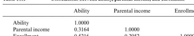
Table 10.1 reports the correlation between ability, observed parental income, and enrollment. All the correlations are signifi cant at more than a 99.9 percent confi dence level. We use the correlation between ability and
enrollment as a calibration target and the correlation between enrollment and parental income as an untargeted prediction of the model.
College Students
For our specifi cation of the expected family contribution function EFC(sY), we use an approximation from Epple et al. (2013) to the true statu-tory formula. Specifi cally, we assume a mapping between raw and adjusted gross parental income of y y( )p = y(1+.07 1[y $50000]) and an EFC for-mula given by EFC(yp)=max{y(yp)/5.5 $5,000,y(yp)/3.2 $16,000,0} in 2009 dollars.
We assume that the government grants (T + ,EFC(sY)) are given by
(12) (T(sY)+ ,EFC(sY))=
F if F T(s
Y)+ EFC(sY)
0 otherwise ,
which refl ects their progressive nature. First, we estimate the average value of government grants from the college- level Integrated Postsecondary Education Data (IPEDS) published by the National Center for Education Statistics (NCES). Then, we calibrate ζF ≥ 1 to match average grants per
student, , in the initial steady state. Over the transition path we keep ζF
constant but vary .
The utility function u(c) = c1–σ/(1–σ) for students as well as workers and
retirees features constant relative risk aversion. We use the standard param-etrization of σ = 2 and β = 0.96. We assume utility from college quality is linear, v (q) = q (and so all curvature comes from the production function
q (θ, I )).
To determine student earnings eY while in college, we again turn to the NLSY97. For our sample, students enrolled in a four- year college earn on average $7,128 (in 2010 dollars).13 We convert this to model units and set eY
equal to it. The mapping from dollars into model units is discussed in the web appendix, section B.1.
Recall that the annual retention rate satisfi es πj+1 = π1[ j + 1 ≤ JY], which implies constant progression probabilities for students in years 1, ,JY 1.
Students in their last year, which we set to JY = 5, successfully graduate and
13. Students work an average of 824 hours a year in the NLSY97. Using diff erent data, Ionescu (2011) reports similar results of 46 percent of full-time students working with mean worker earnings of $20,431 in 2007 dollars.
Table 10.1 Correlations between ability, parental income, and enrollment
Ability Parental income Enrollment
Ability 1.0000 Parental income 0.3164 1.0000
earn a diploma with this same probability. We set = 0.5561/JY to match the
aggregate completion rate of 55.6 percent reported by Ionescu and Simpson (2016).
Last, we allow the nontuition cost of attending college, ϕ, which plays a signifi cant part in determining eligibility for subsidized loans, to vary over the transition path. We measure ϕ using room- and- board estimates from the NCES (NCES 2015c).
Workers/Retirees
The earnings process for working households follows
(13) log eijt = thi/JY + j +zij + zi,j+1= zij + i,j+1
i,j+1~ N(0, 2z)
where hi is the number of completed years of college, i is an individual iden-tifi er, j is age, and t is time. Households who begin working at age j draw zij from an unconditional distribution with mean zero and variance 2z(1 + . . .
+ ρ2( j–1)). For the persistent shock, we use Storesletten, Telmer, and Yaron’s (2004) estimates in setting (ρ, σz) = (0.952, 0.168).14 The deterministic earn-ings profi le μj is a cubic function of age with coeffi cients also taken from Storesletten, Telmer, and Yaron (2004).15
In the model, λt represents the earnings premium for college graduates relative to high school graduates. We compute λt using the estimates from Autor, Katz, and Kearney (2008), which range from roughly 0.43 in the 1960s and 1970s to 0.65 in the early twenty- fi rst century. To deal with the fact that Autor, Katz, and Kearney (2008) estimate values only up until 2005, we fi t a quadratic polynomial over 1988–2005 and extrapolate for 2006–2010.16 We use the fi tted values (both in- sample and out- of- sample) for λt, and they are presented in web appendix A (web appendix B gives a comparison of the raw and fi tted values).
Retired households ( j > JR = 48) have constant earnings given by log eijt = log(0.5) + λthi/JY + JR + v, which yields an average replacement rate of
roughly 50 percent.
10.3.2 Legal Environment and Government Policy
We set the duration of loan repayment to its value in the federal student loan program, tmax = 10. Two parameters—the loan balance penalty η and
14. Storesletten, Telmer, and Yaron (2004) let σ vary with the business cycle and estimate
σ = .211 for recessions and σ = .125 for expansions. We average these.
15. In principle, one could include a cohort-specifi c term that allows for average log earnings in the economy to grow over time. However, we found that such a term is negligible in the data as we show in web appendix B.1.
garnishment rate γ—control the cost of student loan delinquency. Various changes in student loan default laws between 1987 and 2010 render obtain-ing values for these parameters less than straightforward.17 Our approach sets η = 0.05 (which is half the value in Ionescu [2011], and only a fi fth of the current statutory maximum) and then pins down γ in the joint calibration to match the 17.6 percent student loan default rate in 1987.
10.3.3 Colleges
We need to parametrize and provide estimates for the per- student endow-ment E, the quality production function q(θ, I ), and custodial costs F +
C({Nj}JjY=1).
Institution- Level Data
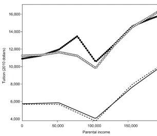
Our primary source for college revenue and expenditures is institution- level data from the Delta Cost Project (DCP), which is drawn from the National Center for Education Statistics Integrated Postsecondary Educa-tion Data System (IPEDS). One important distincEduca-tion between our DCP- based average tuition measures and those reported by the nces330p10y15 (in table 330.10) is that, for public colleges, the NCES only uses in- state tuition.18 Consequently, the gross tuition and fees in our data are larger than those reported by the NCES. However, despite this discrepancy in levels, fi gure 10.1 shows that the trend growth in gross tuition and fees between the two measures is nearly identical.
For sample selection, we restrict attention to four- year, nonprofi t, non-specialty institutions (according to their Carnegie classifi cation) that have nonmissing enrollment and tuition data in every year of the DCP data from 1987 to 2010.19 Additionally, we drop institutions with fewer than 100 FTE students or net tuition per FTE outside of the 1st–99th percentile range.
The college budget constraint in the model features custodial costs, endowment income, quality- enhancing investment, and tuition. The cor-responding data measures are as follows:
• Endowment: total nontuition revenue, which is the sum of (non- Pell) grants at the federal, state, and local levels plus all auxiliary revenue. • Investment: total education and general expenditures including
spon-sored research but excluding auxiliary enterprises. • Tuition: net tuition and fees revenue.
• Custodial costs: a residual computed as the endowment plus tuition less investment.
Web appendix A provides more details on our use of the DCP data.
17. See Ionescu (2011) for changes in student loan default laws.
18. This diff erence in methodologies accounts for the mismatch in reported tuition numbers brought up by our discussant, Sandy Baum.
Calibrated Parameters
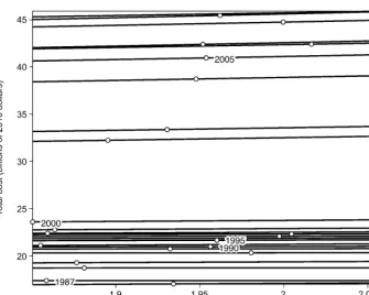
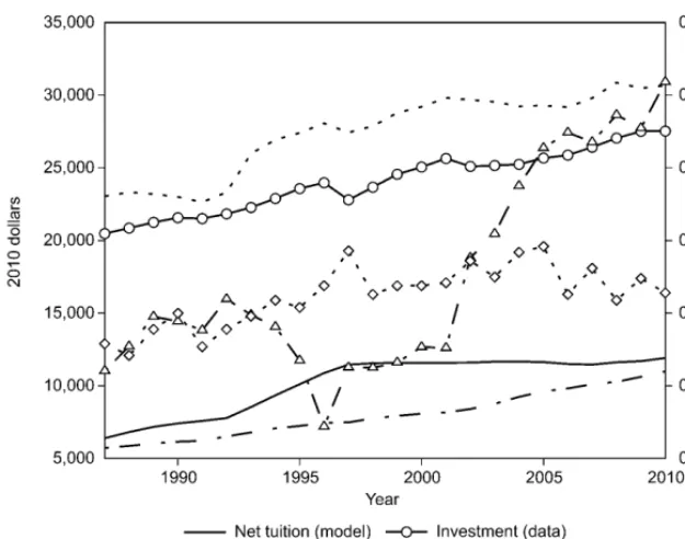
We set the per- student endowment E equal to nontuition revenues per FTE student in the 1987 IPEDS data, and then we vary E along the transi-tion path. Figure 10.2 plots the time series for E and other key aggregates. For college quality, we follow Epple et al. (2013) and choose a Cobb- Douglas functional form, q( , I)= q I I, where χ
I = 1 – χθ.20
The local fi rst- order conditions of the college problem provide some
20. In principle, q (θ, I ) need not satisfy constant returns to scale. With one college, it is diffi cult to pin down—using only steady state information—what the returns should be. With multiple colleges, dispersion in θ and I translates into dispersion in q that is controlled by returns to scale.
A
B
Fig. 10.1 College tuition trends: DCP versus NCES. A, real tuition per FTE;
B, real tuition per FTE, percentage change since 1987.
insight into calibrating χθ and χq. The key tuition- pricing condition comes out to
(14) T s( )Y +
(enroll |sY;T( ),q)
(enroll |sY;T( ),q) / T
=C(N)+I+ q qI
( x(sY))
where (enroll |sY;TsY,q) comes from the decision rule of youths for whether to attend college, taking into account the idiosyncratic preference shock . Epple et al. (2013) label the collected right- hand- side terms the “eff ective marginal cost” (EMC) of a type- sY student, which captures the fact that students act both as customers and as inputs to the production of quality (an argument put forth by Winston [1999] and others). The above equation states that colleges admit any student to whom they can charge at least EMC(sY).
With our Cobb- Douglas specifi cation, qθ/qI = (χθ/χI)(I /θ) = [χθ/(1 –
χθ)](I /θ). The degree to which EMC(sY), and therefore tuition T (sY), varies
by student type depends on χθ. This price discrimination generates cross- sectional enrollment patterns that we use to target χθ and χq. Specifi cally, we target overall enrollment and the correlation between parental income and enrollment.
Cost Function Estimation
Like in Epple, Romano, and Sieg (2006), we estimate the college’s custo-dial cost function directly. In particular, we assume that the custocusto-dial costs by class, c(n), have the functional form C1n + C2n2. When we explicitly allow for time- varying coeffi cients, custodial costs satisfy
(15) Ft+Ct({Njt}JjY=1) =Ft+Ct1 j=1 JY
njt+Ct2 j=1 JY
n2jt
where njt Njt/(1/J) is class j enrollment in year t relative to the age- eighteen population.
To identify Ft, Ct1, and C t
2, we estimate cost functions for individual
col-leges using IPEDS data and then aggregate them. Let college i’s cost function at time t be given by
(16) it = i+ 0t + 1t j=1 JY
nijt+ 2t j=1 JY
nijt2 + it.
Here, αi is a fi xed eff ect and both αi and it are i.d.d. normally distributed
with mean zero.
The IPEDS data contains enrollment information but not its compo-sition by class. To deal with this problem and to create consistency with the model, we assume a constant retention rate π and a fi ve- year college term, JY = 5. Given π, JY, and total FTE enrollment data by school relative to the age- eighteen population, we calculate implied class j enrollment as
nijt = j 1FTEit/ J=Y1 1. Thus, the two summation terms in the cost
func-tion come out to JjY=1nijt = FTEit and JjY=1nijt2 = FTEit2 JjY=1 2(j 1)/( JjY=1 j 1)2.
As a result,
(17) it = i + 0t+ t 1FTE
it+ 2tFTEit2 j=1 JY 2(j 1)
j=1
JY j 1
(
)
2 + it.As in Epple, Romano, and Sieg (2006), we measure custodial costs as a residual in the college budget constraint, which gives us
(18) it it+ it it.
The fi rst term, it, represents total nontuition revenue in IPEDS (which consists mostly of endowment revenue and government appropriations), while it and it equal net tuition revenues and total education and general (E&G) expenditures, respectively. Intuitively, our cost measure refl ects the fact that, holding investment it constant, higher costs must accompany any observed increase in revenues in order to maintain a balanced budget. Using these defi nitions, we run the fi xed eff ects panel regression above to obtain
{(0t, 1t, 2t)}t2010=1987.
of educating {Njt}JjY=1 students, we assume students sort across colleges i = 1,
. . . , K in proportion to the observed share in the data.21 Defi ne s
ijt≡ Nijt/
Njt = nijt/njt as the share of students in class j at time t who attend college i. From our assumption of geometric retention probabilities, this share does not vary with j, that is, sijt = sit. Thus, Nijt = sitNjt and nijt = sitnjt for all j, which gives us22
(19) Ft+Ct({Njt}JjY=1)= K0t + 1t j=1 JY
njt+ 2t i=1
K sit2
j=1 JY
n2jt.
This mapping between individual colleges and the representative college yields Ft = K t0, C
t 1=
t 1, and C
t 2=
t 2
isit 2.
The web appendix presents the estimates. We found it necessary to impose
t
1 =0 to ensure an increasing aggregate cost function over the relevant range
21. We allow K to vary over time in the estimation (it is the number of colleges in the sample) but treat it as fi xed here to simplify the exposition.
22. We assume that i i = 0 and i it = 0, where the fi rst assumption is required for identifi cation in the fi xed eff ects regression.
of N. Figure 10.3 plots the aggregate cost function over time and circles the realized values from each year.
10.3.4 Joint Calibration
We determine the remaining parameters (ν, ξ, γ, χθ, χq, ζF, α) jointly such
that the initial steady state matches the following moments in 1987: average earnings, average net tuition, the two- year cohort default rate, the correla-tion between parental income and enrollment, the enrollment rate, the aver-age grant size, and the percent of students with loans.23
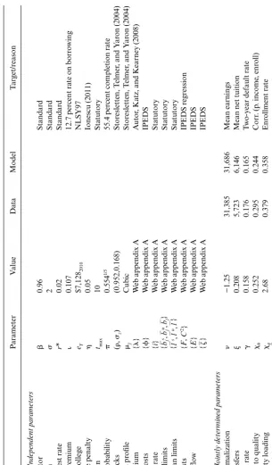
Table 10.2 summarizes the calibration. Note that, while the table associ-ates each parameter in the joint calibration with an individual moment, the calibration identifi es the parameters simultaneously, rather than separately. We discuss model fi t next.
10.3.5 Model Fit
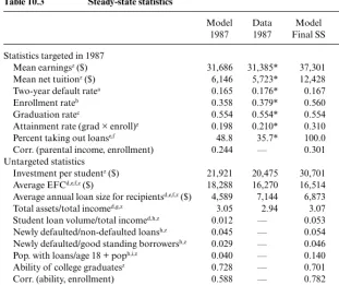
Table 10.3 presents key higher education statistics from the model and the data. The calibration of the initial steady state directly targets the fi rst set of statistics from 1987, while the remaining statistics act as an informal test of the model. Note that, while the calibration matches mean earnings, net tuition, and the two- year default rate from 1987 quite well, the model generates too little enrollment and too many students with loans.
We pinpoint two sources for these shortcomings. First, the presence of only one college in the model generates too much market power, which results in a small calibrated value for the parental transfers parameter ξ in order to still match average net tuition. Thus, students rely more on borrow-ing. Second, by omitting ability terms in the postcollege- earnings process, we implicitly attribute the entire college premium to the sheepskin eff ect of a diploma (as opposed to selection eff ects). This exaggerated sheepskin eff ect generates a larger surplus from attending college, which the college partially captures through higher tuition.
Despite the presence of too many student borrowers, the model actually generates smaller average loans than in the data—$4,600 versus $7,100. Last, the model nearly matches investment per student of $20,300 in 1987 and the ratio of assets to income of about three. The matching of the asset- to- income ratio refl ects the fact that our model of households is, at its core, a standard incomplete markets life- cycle model.
10.4 Results
Now we present the main results. First, we compare the model’s initial and terminal steady states to the data from 1987 and 2010. Next, we evaluate the
T able 10.2 Model calibr ation Description P ar ameter V alue Da ta Model T ar get/r eason Calibr
ation: Independent par
ameter s Discount factor β 0.96 Standar d Risk a v ersion σ 2 Standar d Sa vings inter est r a te r* 0.02 Standar d Borr o wing pr emium ι 0.107 12.7 per cent r a
te on borr
o
wing
Earnings in college
eY
$7,128
2010
NLSY97
Loan balance penalty
η 0.05 Ionescu (2011) Loan dur a tion tmax 10 Sta tutory R etention pr oba bility π 0.554 1/5 55.4 per
cent completion r
a te Earnings shocks ( ρ , σz ) (0.952,0.168) Stor esletten, T elmer
, and Y
ar on (2004) Age- earnings pr ofi le μj Cubic Stor esletten, T elmer
, and Y
ar on (2004) College pr emium { λ } W eb a ppendix A A utor , K a
tz, and K
earney (2008) Nontuition costs { ϕ } W eb a ppendix A IPEDS
Student loan r
a te { i} W eb a ppendix A Sta tutory Ann
ual loan limits
bj
s,b
j u, bj {} W eb a ppendix A Sta tutory Aggr ega
te loan limits
l
s,l u, l {} W eb a ppendix A Sta tutory Custodial costs { F , C 2} W eb a ppendix A IPEDS r egr ession Endo wment fl ow { E } W eb a ppendix A IPEDS Gr ant aid {} W eb a ppendix A IPEDS Calibr ation: J ointl
y determined par
ameter s Earnings nor maliza tion ν −1.25 31,385 31,686 Mean earnings P ar ental tr ansfers ξ 0.208 5,723 6,146
Mean net tuition
Garnishment r a te γ 0.158 0.176 0.165 T w o- y
ear default r
a
te
Ability input to quality
χθ 0.252 0.295 0.244 Corr . (p . income , enr oll)
College quality loading
χq 2.68 0.379 0.358 Enr ollment ra te Gr ant pr o gr essi vity ζ F 1.85 0.027 0.025 A v er a ge gr ant siz e Pr efer
ence shock siz
e α 290 0.357 0.488 P er
cent with loans
Note:
{
x
} means
x
has a tr
ansition pa
th gi
v
en in ta
b
le 2 in w
eb a
ppendix A; $
xyyyy means $ x , measur ed nominall y in yyyy dollars , con v