SPECIAL ISSUE: The Dynamics and Value of Ecosystem Services: Integrating
Economic and Ecological Perspectives
Modeling the dynamics of the integrated earth system and
the value of global ecosystem services using the GUMBO
model
Roelof Boumans
a,*
,1, Robert Costanza
a,1, Joshua Farley
a,1,
Matthew A. Wilson
a,1, Rosimeiry Portela
b, Jan Rotmans
c,
Ferdinando Villa
a,1, Monica Grasso
daInstitute for Ecological Economics,Uni6ersity of Maryland,Solomons,MD,20688,USA
bMarine,Estuarine and En6ironmental Science Program,Uni6ersity of Maryland,College Park,MD20742,USA cInternational Center for Integrati6e Studies,Maastricht Uni6ersity,
6200MD Maastricht,The Netherlands dIndependent Consultant,239Rawson Road,
c5,Brookline,MA02446,USA
Abstract
A global unified metamodel of the biosphere (GUMBO) was developed to simulate the integrated earth system and assess the dynamics and values of ecosystem services. It is a ‘metamodel’ in that it represents a synthesis and a simplification of several existing dynamic global models in both the natural and social sciences at an intermediate level of complexity. The current version of the model contains 234 state variables, 930 variables total, and 1715 parameters. GUMBO is the first global model to include the dynamic feedbacks among human technology, economic production and welfare, and ecosystem goods and services within the dynamic earth system. GUMBO includes modules to simulate carbon, water, and nutrient fluxes through theAtmosphere,Lithosphere,Hydrosphere, andBiosphereof the global system. Social and economic dynamics are simulated within the Anthroposphere. GUMBO links these five spheres across eleven biomes, which together encompass the entire surface of the planet. The dynamics of eleven major ecosystem goods and services for each of the biomes are simulated and evaluated. Historical calibrations from 1900 to 2000 for 14 key variables for which quantitative time-series data was available produced an averageR2of
0.922. A range of future scenarios representing different assumptions about future technological change, investment strategies and other factors have been simulated. The relative value of ecosystem services in terms of their contribution to supporting both conventional economic production and human well-being more broadly defined were estimated under each scenario, and preliminary conclusions drawn. The value of global ecosystem services was estimated to be about 4.5 times the value of Gross World Product (GWP) in the year 2000 using this approach. The model can be downloaded and run on the average PC to allow users to explore for themselves the complex dynamics of the system and the full range of policy assumptions and scenarios. © 2002 Elsevier Science B.V. All rights reserved.
Keywords:GUMBO model; Integrated earth system; Global ecosystem
This article is also available online at: www.elsevier.com/locate/ecolecon
* Corresponding author. Tel.: +1-410-326-7281; fax: +1-410-326-7354 E-mail address:[email protected](R. Boumans).
1As of 09/01/2002, this author can be reached at the Gund Institute for Ecological Economics, University of Vermont, School
R.Boumans et al./Ecological Economics41 (2002) 529 – 560
530
1. Introduction
There is now a relatively long history of global computer simulation modeling, starting in the 1970s with the World2 (Forrester, 1971) and World3 models (Meadows et al., 1972; Meadows and Meadows, 1975). Since then the field has expanded greatly, owing partly to the increasing availability and speed of computers and to the rapidly expanding global data base that has been created in response to increased interest in global climate change issues (Meadows, 1985; Meadows et al., 1992; Nordhaus, 1994; Rotmans and de Vries, 1997; IPCC, 1992, 1995, 2001). Collectively, global models constitute a relatively well focused and coherent discussion about our collective fu-ture. As Meadows (1985) has pointed out:
‘‘Global models are not meant to predict, do not include every possible aspect of the world, and do not support either pure optimism or pure pessimism about the future. They repre-sent mathematical assumptions about the inter-relationships among global concerns such as
population, industrial output, natural
re-sources, and pollution. Global modelers
investi-gate what might happen if policies continue
along present lines, or if specific changes are instituted’’ (Meadows 1985, p. 55; Italics added).
The global unified metamodel of the biosphere (GUMBO), which we describe in this paper, builds on the long tradition of global modeling and the rapidly expanding global data base.
GUMBO addresses the following key
objectives:
1. To model the complex, dynamic interlinkages between social, economic and biophysical sys-tems on a global scale, focusing on ecosystem goods and services and their contribution to sustaining human welfare.
2. To create a computational framework and data base that is simple enough to be dis-tributed and run on a desktop PC by a broad range of users. GUMBO was constructed in STELLA, a popular icon-based dynamic
simu-lation modeling language (http://www.hps
-inc.com), and the full model can be
downloaded and run using the free run-time only version of STELLA.
In designing GUMBO we sought to provide a flexible computational platform for the simulation of alternative global pasts and futures envisioned by diverse end-users. GUMBO limits historical parameter values to those which produce histori-cal behavior consistent with historihistori-cal data. It then allows one to make explicit assumptions about future parameter or policy changes, or to determine what assumptions are required to achieve a specific future. It is then possible to assess how plausible those assumptions are, and to consider policy options that might make the assumptions required for a desired future more likely to occur. By allowing the user to change specified parameters within GUMBO and gener-ate alternative images of the future we hope to provide a tool that will both stimulate dialogue about global change and generate a more com-plete understanding of the complex
interrelation-ships among social and economic factors,
ecosystem services, and the biophysical earth sys-tem. This dialogue is needed in order to achieve sustainable development on a global scale.
GUMBO is unique among global models in three important ways:
1. ecosystem services are a focus of GUMBO and explicitly affect both economic production and social welfare. This allows the model to calcu-late dynamically changing values for
ecosys-tem services based on their marginal
contributions relative to other inputs into the production and welfare functions.
2. both ecological and socioeconomic changes are endogenous to the model, with a pro-nounced emphasis on interactions and feed-backs between the two — all other global models to date limit either ecological or so-cioeconomic change to exogenously deter-mined scenarios (c.f. Meadows et al., 1992; Rotmans and de Vries, 1997; IPCC, 2001); 3. the model includes natural capital, human
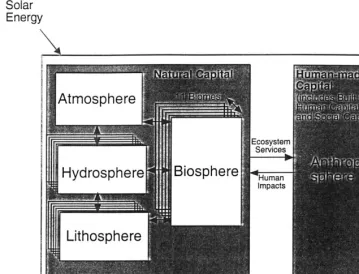
Fig. 1. Basic structure of GUMBO. The hydrosphere, lithosphere, and biosphere are reproduced for each of 11 biomes. STELLA diagrams to indicate the general complexity of the structure of each sphere are given in Figs. 2 – 9. The full model and equations are available for download at: http://iee.umces.edu/GUMBO.
of transformation (material cause and efficient cause, in Aristotelian terms). Thus, the model allows limited substitution between factors of production at the margin, but also imposes strong sustainability constraints for the system as a whole.2
This paper first describes the general structure and behavior of GUMBO, along with limitations and caveats (the full model and documentation
can be downloaded from: http://iee.umces.edu/
GUMBO). It then presents results from a few
alternative scenarios developed using contrasting assumptions about technology, the resilience of the global environmental system and the ability of economic production to cope with future changes in sinks and sources of natural capital. For each scenario, we examine the dynamics of the values of ecosystem services to assess which ecological variables impose the tightest constraints on pro-duction and welfare. We also discuss the plausibil-ity of the assumptions necessary to bring about each scenario, and the level of risk implied in planning futures around each scenario.
2. Model development
GUMBO consists of five distinct modules or ‘spheres’: the Atmosphere, the Lithosphere, the Hydrosphere, the Biosphere, and the
Anthropo-2Weak sustainability requires that the future be left a
R.Boumans et al./Ecological Economics41 (2002) 529 – 560
532
sphere (Fig. 1). It is further divided into 11 biomes or ecosystem types which encompass the
entire surface area of the planet: Open Ocean,
Coastal Ocean, Forests, Grasslands, Wetlands,
Lakes/Ri6ers, Deserts, Tundra, Ice/rock, Crop
-lands, and Urban (see Fig. 1). These 11 biomes represent an aggregation of the sixteen biomes used in Costanza et al. (1997a). Their relative areas change in response to urban and rural pop-ulation growth, Gross World Product (GWP), and changes in global temperature. Among the spheres and biomes, there are exchanges of en-ergy, carbon, nutrients, water and mineral matter. GUMBO is the first global model to explicitly account for ecosystem goods and services and factor them directly into the process of global economic production and human welfare develop-ment. Ecosystem services contribute to human quality of life in numerous ways. First, such ser-vices provide critical life-support systems for hu-mans and all other species. Second, all sustainable production processes require renewable resource inputs. By creating the conditions essential for the reproduction of all forms of life, ecosystem ser-vices also provide the material means for sustain-able economic production. Third, ecosystem services create the conditions necessary for culti-vated natural capital, such as agriculture, aqua-culture and silviaqua-culture. Ecosystem services also contribute directly to human well-being (Daily, 1997; Costanza et al., 1997a). In GUMBO, ecosystem services are aggregated to seven major types, while ecosystem goods are aggregated into four major types. Ecosystem services, in contrast to ecosystem goods, cannot accumulate or be used at a specified rate of depletion. Ecosystem services include: soil formation, gas regulation, climate regulation, nutrient cycling, disturbance regula-tion, recreation and culture, and waste assimila-tion. Ecosystem goods include: water, harvested organic matter, mined ores, and extracted fossil fuel. These 11 goods and services represent the output from natural capital, which combines with built capital, human capital and social capital to produce economic goods and services and social welfare.
Below we briefly describe the major ‘sectors’ in the GUMBO model. The atmosphere and
anthro-posphere are considered to be globally
homoge-nous in this version. The other sectors
(lithosphere, hydrosphere, and biosphere) are di-vided into 11 biomes and the structure described is replicated for each biome. In addition, there are sectors in the model for ecosystem services, land use, and the model’s data base. In what follows, we briefly describe the important processes and structure in each sector and display the STELLA diagram for the sector to indicate how the ele-ments are connected. In these diagrams, boxes represent state variables, double arrows represent fluxes in and out of state variables, single arrows represent information flows or other functional connections, and circles represent auxiliary vari-ables. The full model with equations and
docu-mentation is available for download at:
http://iee.umces.edu/GUMBO.
2.1. The atmosphere
The atmosphere module in GUMBO (Fig. 2) facilitates exchanges of carbon, water, and nutri-ents across biomes. The atmosphere also accounts for global energy balances. Atmospheric dynamics are calibrated against two important global
indi-cators: atmospheric carbon and global
temperature.
Source and sink functions of atmospheric car-bon are linked to all other spheres. For example, carbon exchange with the biosphere depends on the rates at which carbon is lost to the atmo-sphere from burning and decaying plant material as well as the rates of carbon removal from the
atmosphere through vegetation growth
(Houghton et al., 1987). Carbon exchange with the lithosphere occurs through degassing from volcanic activity, and the accumulation and oxi-dation of organic soil matter (Houghton et al., 1987). The net carbon flux between the atmo-sphere and the hydroatmo-sphere results from partial pressure differences between air and water. Car-bon input from the anthroposphere to the atmo-sphere is primarily the result of fossil fuel combustion and cement production.
atmospheric nutrients, primarily various types of nitrogen oxides, are introduced from biomass oxi-dation in the biosphere and fossil fuel combustion within the anthroposphere. Atmospheric nutrient sinks are ocean sea spray and wet precipitation in the hydrosphere and dry deposition in the lithosphere.
Global energy accounting was adapted from a
model created by Few (ftp.usra.edu/pub/esse/
DROP/outgoing/stella/few/energymod3.stm) in order to simulate energy budgets for each biome at 1-year time steps. We introduced spatial energy diffusion fluxes to account for heat exchanges across biomes. Incoming solar energy is propor-tional to a solar radiation constant and a biome-specific albedo. Energy radiation into space is proportional to biome-specific properties for heat retention and imperfect emissivity. Energy ex-changes between biomes take into account tem-perature differences and time constraints for energy transport.
2.2. The lithosphere
The GUMBO lithosphere (Fig. 3) represents the solid uppermost shell of the earth, which includes soils and deposited sediments. Litho-sphere stocks are represented by silicate rocks, carbon reserves, and ore and fossil fuel deposits in rock and soil. Fluxes between rocks and soils are from weathering and sedimentary deposition (burial). New silicate rock is formed and lost by the slow rates of ocean spreading and seafloor subduction. Weathering causes an overall decay of carbon, silicate rocks and ore deposits and forms soils through interaction with the bio-sphere. A specified ‘burial rate’ converts carbon, silicates and ores back into sedimentary rocks and accounts for biome-specific recycling rates.
2.3. The hydrosphere
The GUMBO hydrosphere (Fig. 4) accounts for biome-specific stocks of water, carbon, and ‘generic nutrients’ in surface and subsurface water bodies. Surface storage occurs in ice and surface water, subsurface storage occurs in deep water, fossil water and unsaturated water (soil moisture). Storage of carbon and nutrients in the hydro-sphere occur in surface water, terrestrial ground-water and oceanic surface and deep ground-water. Average biome temperature determines the nature of precipitation. Fluctuating biome temperatures from the atmospheric energy module regulate the water exchange between ice and surface waters. Surface water exchanges between continental and
R.Boumans et al./Ecological Economics41 (2002) 529 – 560
534
Fig. 3. STELLA diagram of the Lithosphere sector.
oceanic biomes are calculated to compensate for uneven distributions among biome-specific evapo-transpiration. Additional fresh water is available as ‘fossil water’ stored in geological deposits and does not normally have free exchange with surface waters. GUMBO allows the mining of fossil water as a reaction to shortages in surface water due to the demand for water generated in the anthropo-sphere. Biome-specific stocks of nutrients are ex-changed with the atmosphere (e.g. nitrogen fixation and denitrification), the lithosphere (e.g. erosion and sedimentary processes), and the bio-sphere (e.g. mineralization and plant uptake).
2.4. The biosphere
The biosphere is a self-regulating system sus-tained by large-scale cycles of energy and materi-als such as carbon, oxygen, nitrogen, certain minerals, and water. The fundamental processes
R.Boumans et al./Ecological Economics41 (2002) 529 – 560
536
carbon in the biosphere that resides in the dead organic matter is fluxed towards soil formation and ultimately towards the formation of carbon deposits in rock.
Many of the ecosystem services provided by the biosphere are associated with the rate of photo-synthesis or productivity of autotrophs. Impor-tant factors for achieving optimum productivity are the nutrient availability in the lithosphere, temperature, light levels, and carbon pressure in the atmosphere, soil moisture in the hydrosphere
and waste levels generated within the
anthroposphere.
2.5. The anthroposphere
The anthroposphere in GUMBO (Fig. 6) repre-sents human social and economic systems. The anthroposphere harvests large amounts of mate-rial and energy from the larger system and dis-cards waste at each phase along a production chain. In contrast to the larger biosphere, only a very small portion of materials are internally recy-cled within the anthroposphere. Human popula-tion, knowledge and social institutions (rules and norms) drive the rate of this material and energy flux.
The anthroposphere is the nexus of valuation in GUMBO. The anthroposphere brings together the numerous elements within the other spheres that affect human well-being, links them to hu-man activities that affect well-being, and assesses the impacts of human activity on those elements. There are two distinct types of value estimated in GUMBO. First, GUMBO calculates the contribu-tion of the elements, activities and impacts to the production of conventional economic goods and services (GWP). Second, GUMBO calculates the contribution of the elements, activities and im-pacts to our sustainable social welfare (SSW) function or quality of life. Both economic produc-tion and human welfare are modeled with a Cobb – Douglas function, as follows:
GWP=HKh1· SKh2· BKh3· Wh4·5 i=1 10 NK
i hi+4
and
SSW=BKi1· Ci2·5 i=1 7 NK
i
ii+2· HKi10· SKi11
· Wi12· Mi13
where
hn and in are the percentage increases in levels
of output (GWP or SSW, respectively) arising from a 1% increase in the corresponding input.
Inputs are: HK=human capital (technology and
labor), SK=social capital (social networks and
institutions), BK=built capital (buildings, roads,
etc.), W=waste (waste products of depreciated
capitals and consumption), C=consumption
(non-invested GWP), NK=natural capital
(dis-aggregated into the 11 ecosystem goods and
ser-vices), and M=mortality. The coefficients on
waste,h4 and i4, and Mortality i13 are negative,
while all others are positive. The hi and ii
parameters are different for the production and welfare function. Differences between the produc-tion and welfare funcproduc-tions are that the welfare function: (1) includes only ecosystem services (not ecosystem goods like fossil fuel); and (2) it also includes C (which is a percentage of the produc-tion funcproduc-tion), and M (average human death rate as an indicator of human health). Thus the wel-fare function includes the welwel-fare derived from production (via consumption) plus the welfare derived directly from the non-marketed ecosystem services, social capital, built capital, and human capital, and the negative influences on welfare of waste and mortality. Distribution effects on wel-fare are included through the influence of social capital (Putnam, 2000).
While thehiparameters in the production
func-tion can be calibrated to fit GWP data, values of the ii parameters in the welfare function are, of
course, matters of aggregate individual prefer-ences, which are themselves moderated through culture and world view. In GUMBO we allow the
user to experiment with these weights and/or to
R.Boumans et al./Ecological Economics41 (2002) 529 – 560
538
assume 20% optimists (mainly populating the de-veloped world) and 80% skeptics. The optimists give more weight to built capital, consumption, and individual knowledge, and less to natural capital and waste. Both weigh social capital and mortality equally.
The Cobb – Douglas function adopted here is among the most widely used functions in eco-nomic modeling for a number of reasons. First the marginal product of each input is positive and decreasing. That is, more of any input will always lead to more output, but each additional unit of input produces less additional output than the preceding one, if other inputs are held constant. Second, it allows for substitution between inputs. Third, and probably most importantly, it is math-ematically tractable and log linear, leading to ease of estimation and manipulation (Bairam, 1994).
A limitation of the Cobb – Douglas function in some models is that it allows a virtually infinite substitution of inputs. As long as no input goes to zero, more of any input can always substitute for less of another. This is equivalent to the notion of weak sustainability, which assumes that more built (or social or human) capital can always substitute for less natural capital. However, there are powerful arguments for assuming strong sus-tainability (i.e. beyond some threshold built, hu-man or social capital cannot substitute for natural capital). For example, no number of fishing boats
can substitute for drastically depleted fish stocks.
But the GUMBO model is a systems model that
captures the feedbacks between the use of capital stocks in the production function and the produc-tion of the capital stocks themselves. In GUMBO the notion of strong sustainability is thus explic-itly built in because natural capital is an essential input to all other forms of capital. There is no economic ‘production’ in the model, only formation. Natural capital is the material trans-formed, while built, social and human capital are the agents of transformation. Thus, while more built capital, social capital or human capital can substitute for less natural capital in the tion of GWP or SSW at the margin in the produc-tion funcproduc-tion, these capitals themselves cannot be produced without natural capital. Thus natural capital is fundamentally a complement to the other capitals in the production process. Further, if natural capital falls below a certain level, or if waste emissions reach excessive levels, natural capital loses the ability to regenerate in the model, and begins a spontaneous decline. Once such a threshold is passed, natural capital can fall to zero, at which point production could fall to zero regardless of the level of other inputs. This ap-proach effectively models the principles of strong sustainability.
The GUMBO framework permits the quantita-tive aggregation of ‘factors of production’ con-tributing to both GWP and SSW into four distinct types of capital stocks: natural capital,
social capital, human capital and built capital(see
Berkes and Folke, 1994; Serageldin, 1996;
Costanza et al., 1997b, 2001).
2.6. Natural capital
Natural capital aggregates all the biophysical stocks which produce both ecosystem goods (raw materials and mineral resources) and ecosystem services. Both ecosystem goods and services con-tribute to both GWP and SSW. Ecosystem goods are the only source of material means, and hence are essential inputs into all production processes, human or natural, but also contribute directly to our quality of life independent of their contribu-tion to produccontribu-tion. Unlike the other forms of
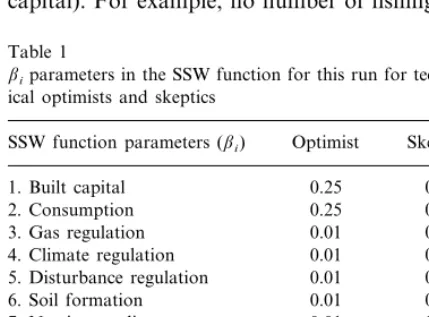
Table 1
iiparameters in the SSW function for this run for technolog-ical optimists and skeptics
Skeptic Optimist
SSW function parameters (ii)
1. Built capital 0.25 0.01
0.01
2. Consumption 0.25
0.05 0.01
3. Gas regulation
0.01
4. Climate regulation 0.05
5. Disturbance regulation 0.01 0.05
6. Soil formation 0.01 0.05
0.01
7. Nutrient cycling 0.05
0.01 0.05
8. Waste treatment
0.10 0.04
9. Recreational and cultural
0.35
10. Knowledge 0.10
2.00
11. Social capital 2.00
12. Waste −0.01 −0.50
−0.20
R.Boumans et al./Ecological Economics41 (2002) 529 – 560
540
capital, natural capital is capable of reproduction on its own with no human intervention. Thanks to the steady inflow of solar energy, it is possible to invest in renewable natural capital simply by using it up slower than it replenishes itself. It is also possible to actively invest in natural capital through ecological restoration, or to cultivate nat-ural capital with inputs of human, social and built capital. Within GUMBO, we invest goods and services in natural capital by reducing
con-sumption and/or direct investment via ecosystem
protection and restoration efforts.
2.7. Social capital
Social capital refers to the institutions, relation-ships, and norms that shape the quality and quantity of a society’s social interactions. Social capital is not just the sum of the institutions that underpin human society; it is the glue that holds
them together (http://www.worldbank.org/
poverty/scapital/whatsc.htm). Social capital re-duces transaction costs via cooperation and makes social and economic interactions possible (Costanza et al., 2001). It is thus an essential element in virtually all economic production, but that is only a part of the benefit it provides as it contributes directly to SSW. Humans are innately social creatures, and human relationships, trust and community are essential components of our SSW. While social capital can depreciate, it does not wear out through use. Indeed, it would seem that using social capital probably increases it, while neglecting it leads to its decay. However, it is also likely that building excess social capital within a group (bonding) can make it more difficult to establish social capital between groups (bridging) (Putnam, 2000). While seemingly im-material, social capital cannot, of course, exist without people, human contact, and appropriate infrastructure, all of which require material in-puts.
2.8. Human capital
Human capital consists of both quantity and quality of technology, knowledge and labor. As a
critical factor in the quality of labor, health is also a component of human capital. Production of any sort is impossible without labor and knowledge. Human capital in the form of ac-quired knowledge, skills and physical health fur-ther contributes to our SSW. An education, it has been said, makes your mind a better place to spend your leisure time. Skills and knowledge instill pride and status, and offer greater opportu-nities for less dangerous, more fulfilling employ-ment. And few would deny that health plays an important role in SSW.
In GUMBO, human technology is represented simply as the overall stock of human knowledge. As such, human capital can depreciate if not used, or it can be stored in various formats. Each of these formats, of course, requires material and energy to create and maintain, and hence requires continual investment in order not to depreciate. Future generations must also be trained in how to access and use this stored information. In
addi-tion, as new knowledge accumulates, older
knowledge often becomes obsolete, which is also a form of depreciation.
2.9. Built capital
Built capital and labor have traditionally re-ceived the greatest attention in economic analysis. No explanation is necessary concerning how built capital contributes to GWP and how it requires resources for creation and maintenance. While built capital also contributes directly to SSW (the sole purpose of any aesthetic architectural embel-lishments, for example), it may play a less impor-tant role than is often assumed (Frank, 1999). Built capital continues to play a major role, how-ever, in the depletion of resources, and in the current economic system, ownership of built capi-tal strongly influences the distribution of wealth. Of all the capitals, investment in built capital places the most demands on natural resources. Built capital depreciates by physically falling apart, or else as the result of new technologies making existing infrastructure obsolete.
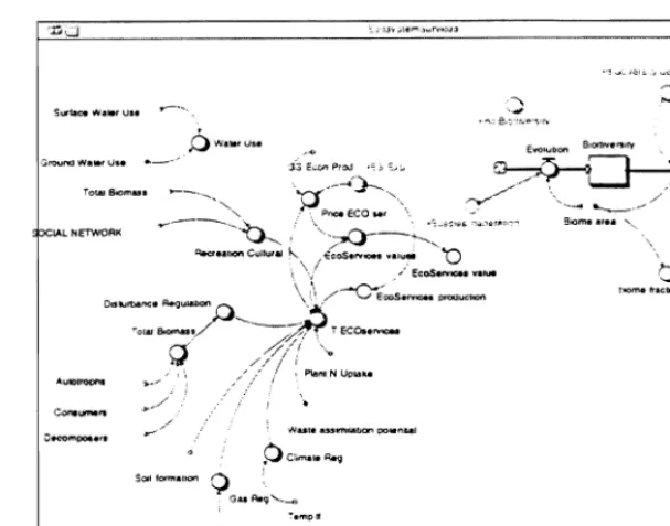
Fig. 7. STELLA diagram of the Ecosystems services sector.
within the anthroposphere even though they make different contributions to each. In GUMBO, ac-cumulated waste reduces the output of both GWP and SSW. Consumption contributes to SSW. Hu-man, social and built capital stocks spontaneously depreciate, while natural capital is renewable and has the potential for self-maintenance. Aggregated economic goods and services (GWP) can be in-vested in maintaining or creating any of the four capitals, or can be consumed. Investment in hu-man, social or built capital requires a fixed amount of GWP and of raw materials, though it is possible to allow raw material demands to change with changing technology. Rates of invest-ment in each type of capital are control variables in the model. Consumption depreciates instantly into waste, and social, human and built capital become waste as they depreciate over time. Waste absorption capacity is an ecosystem service, and if the flow of waste is greater than the absorption capacity, waste accumulates. Waste accumulation (i.e. pollution) directly affects the ability of natu-ral capital to spontaneously reproduce, and can even cause it to spontaneously degrade. It also decreases production of GWP and SSW.
2.10. Ecosystem ser6ices
The 17 ecosystem services listed in Costanza et al. (1997a) have been aggregated somewhat in GUMBO and some were not included. Seven classes of ecosystem services are included in GUMBO (Fig. 7) and are briefly described below. A more complete classification and description of ecosystem services and functions is available in de Groot et al. (this volume). In what follows we briefly describe how each class of service is in-cluded in GUMBO.
2.10.1. Gas regulation
Gas regulation refers to the regulation of atmo-spheric chemical composition (Costanza et al., 1997a). In GUMBO, this ecosystem service is primarily associated with the changes in the global C cycle — exchanges of carbon within the biosphere and primary productivity of the bio-sphere terrestrial and ocean biomes. The exchange of C is simulated as processes such as terrestrial
respiration, fossil fuel extraction, degassing,
R.Boumans et al./Ecological Economics41 (2002) 529 – 560
542
2.10.2. Climate regulation
This service is defined as the regulation of global temperature, precipitation, and other biologically mediated climatic processes at global or local levels (Costanza et al., 1997a). In GUMBO, climate regulation is associated with variations in global temperature from year to year. A global biome energy pool determines global average tempera-ture. An inflow of solar radiation to the Earth and an outflow of radiation from the Earth to space controls this energy pool, and the energy pool is in turn affected by the extent of biome area, their albedo capacity and by the atmospheric C pool.
2.10.3. Disturbance regulation
This service is described as an ecosystem’s capac-itance, damping and resilience in response to envi-ronmental fluctuations (Costanza et al., 1997a). In the GUMBO model, it is measured as the biome’s yearly change of total biomass (autotrophs, con-sumers and decomposers). The lower the variability in biomass, the greater the systems’ disturbance regulation service.
2.10.4. Soil formation
Soil formation results from the weathering of rock material and of the accumulation of organic matter (de Groot et al., 2002). In GUMBO, the process of soil formation is closely related to rates of decomposition (Schlesinger, 1997), thereby ac-counting for different rates of organic matter accumulation in different biomes. As autotrophs and consumers die, a pool of dead organic matter accumulates, and from this pool a flux of soil formation is generated in each biome.
2.10.5. Nutrient cycling
This service refers to the storage, cycling, pro-cessing and acquisition of nutrients within the global system (Costanza et al., 1997a). In GUMBO, Nitrogen is used as a proxy for all other nutrients, and plant uptake of N serves as a proxy for nutrient cycling. Plant N uptake is represented as an inflow of nutrients into the soil nutrient pool associated with each biome’s gross primary produc-tion, soil formation and biomass nutrient content. The soil nutrient pool also is influenced by atmo-spheric exchanges, weathering of rock material and fertilizer application.
2.10.6. Waste assimilation
This service refers to nature’s ability to recover mobile nutrients, and remove or breakdown excess xenic nutrients and compounds (Costanza et al., 1997a). In GUMBO, this is modeled as the product of waste stock and either waste assimilation rate or waste assimilation potential — the model chooses the lowest value from the two. In each time step assimilation potential is represented as total assim-ilation capacity relative to the current amount of waste.
2.10.7. Recreational and cultural
These services hinge on an ecosystem’s ability to provide for recreational activities such as eco-tourism and sport fishing as well as cultural activ-ities like worship and aesthetic appreciation (Costanza et al., 1997a). In the GUMBO model, recreational and cultural activities are positively related to total biomass amounts and the density of the social network, and negatively related to human population stocks. Hence, while the recre-ational and cultural activities service increases with increasing social network density and biomass, it decreases with increasing population.
2.11. ‘Prices’ of ecosystem ser6ices: marginal products as a measure of 6alue
While future versions of the GUMBO model will include a variety of methodologies for calcu-lating ecosystem values,3 the current version
cal-3For example, the ‘simplest’ approach to pricing ecosystem
culates the marginal product of ecosystem ser-vices in both the model’s production and welfare functions. The rationale is simple. We calculate the impact of an incremental change in an ecosystem service on total output (either produc-tion of goods and services or of welfare). For example, if an additional unit of ‘climate stabil-ity’ (measured as reduced variability around a mean temperature) increases global output by $3 million, then climate stability must be worth $3 million per unit at the margin under current conditions. We will refer to these estimates of marginal product as ecosystem service prices. Conditions for calculating ‘theoretically correct’ prices using this approach include optimal allo-cation of all resources, no externalities, and no public goods. However, we are not interested in theoretical prices in some fictitious ‘optimal’ world, but rather in what the world would be willing to pay for an extra unit of that service under actual conditions in the current time pe-riod, given the existing allocation of other re-sources — and this is precisely what the marginal contribution of an ecosystem service to global production or social welfare tells us. In addition, GUMBO is a global model in which externali-ties and property rights (and hence the public good issue) are irrelevant with respect to prices. Further, within the model, we know resource stocks, and deterministic model equations are equivalent to complete knowledge concerning system-wide impacts of resource use. Hence, while the assumptions necessary for the marginal analysis approach to pricing rarely hold in the real world, they do approximately hold in the world of the GUMBO model (which is one of the main reasons for constructing the model in the first place).
Another important point is that the appropri-ate price for ecosystem services is the current time marginal product of the service, not includ-ing the value of the given service in future time periods. We make an important distinction be-tween environmental goods that are produced from ecosystem structure and ecosystem services that result from ecosystem function. Without ecosystem structure there is, of course, no
ecosystem function, but the two components of natural capital have quite different physical and economic properties and must be treated sepa-rately. Ecosystem goods are in the form of stocks and flows: a stock of trees generates a flow of wood products, a stock of fish generates a flow of fish protein, and a stock of grass erates a flow of fodder. These goods are in gen-eral both rival (if one person benefits from the good, another cannot) and excludable (it is pos-sible to exclude people from benefiting from them), and in the absence of negative externali-ties from their use, could be suitably allocated by market forces. Ecosystem services are in the form of funds and services: the stocks found in a forest (ecosystem structure) interact to gener-ate the services of climgener-ate regulation, gas regula-tion and water regularegula-tion (ecosystem funcregula-tion). Services cannot accumulate into stocks or funds, so in calculating the price for a service, it would be a mistake to consider costs or benefits derived from that service in future periods. In the future we will use GUMBO to value both natural capital stocks and funds, and in this case will need to account for flows and services in future periods. Note also that most ecosystem services are both non-rival and non-excludable and hence they cannot be efficiently allocated by unregulated market forces. Waste absorption ca-pacity is an important exception, as it is rival, and can be made excludable.
R.Boumans et al./Ecological Economics41 (2002) 529 – 560
544
to price, and change this one by a small
incre-ment.4 The measured change in the value of the
output will be equal to the price of the increment of the variable in question. With the latter ap-proach, we are free to use the most appropriate function to model a particular process. In the current version of the model, we have taken the simpler approach of mathematically approximat-ing first derivatives.
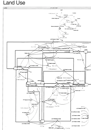
2.12. Land use
Eleven land (and water) use/cover types (or
biomes) are included in GUMBO (Open Ocean, Coastal Ocean, Forests, Grasslands, Wetlands, Lakes/Rivers, Deserts, Tundra, Ice/rock, Crop-lands, and Urban). Land use changes in GUMBO (Fig. 8) are driven by human population and GWP changes (from the anthroposphere), con-strained by the remaining area of each biome. Population is partitioned into urban and rural components.
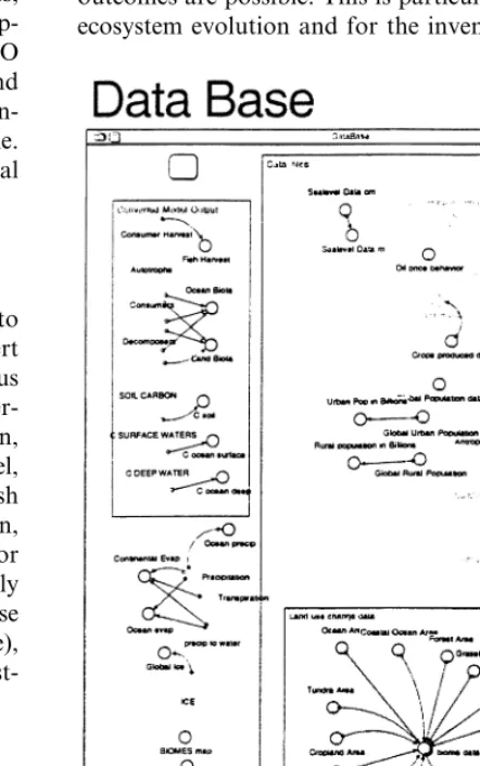
2.13. Data base
A separate sector is included in GUMBO to store the calibration data for the model, convert units as necessary, and do other miscellaneous conversions (Fig. 9). Global data includes:
aver-age temperature, atmospheric CO2concentration,
anthropogenic CO2production, average sea level,
GWP, human population, oil production, fish
harvest, food production, forest production,
metals and minerals production, and land use for each of the 11 biomes. Our plan is to ultimately link the model to an integrated on-line data base that we are creating (see Villa et al., this volume), which will allow continuing recalibration and test-ing of the model.
2.14. Limitations and ca6eats
Like any model, GUMBO only represents a simplified description of the world and has the
same general limitations shared by all global mod-els. Because ‘simplification is the essence of model building’, there will always be issues that remain outside the purview of the model (Meadows and Meadows, 1975, p. 17). For example, we remain largely ignorant of precisely how ecosystem struc-ture generates ecosystem services, and must in-stead rely on the best accepted and most plausible explanations present in the literature to model these complex relationships (see de Groot et al., this volume). Some of the changes important to GUMBO are characterized by pure uncertainty — we are ignorant not only of the probabilities of various outcomes, but we do not even know what outcomes are possible. This is particularly true for ecosystem evolution and for the invention of new
Fig. 9. STELLA diagram of the Data Base sector.
4To do this efficiently, we would feed the output of the
R.Boumans et al./Ecological Economics41 (2002) 529 – 560
546
human technologies, both of which are critical factors determining the impact of human action on ecosystem services. As we describe later, these uncertainties are handled using alternative future scenarios that allow the implications of alternative assumptions to be explored. Another serious chal-lenge involves investments in productive capacity within the economic sub-system. Most global models have greatly simplified economic produc-tion within the model by either leaving out price-investment feedback loops (Meadows et al., 1972, 1992), or by treating economic production as exogenous to the system (Rotmans and de Vries, 1997). In GUMBO, relative rates of investment are currently treated as exogenous control vari-ables manipulated by the model user. In addition, the functional forms we have chosen for both the GWP and SSW functions (see Section 2.5) are relatively simplistic and the variable coefficients are somewhat subjective. However, a major strength of the GUMBO model is that users can readily manipulate these functions and variables and observe the resulting impacts on the model output.
3. Results
In this section, we describe both the preliminary calibration results for the model and the results of a series of scenarios. These results are summarized in Figs. 10 – 15. The model was run starting in 1900 for 200 years at a time step of 1 year. Each figure shows a selection of related variables over the historical period from 1900 to 2000, and con-tinuing over the future period from 2000 to 2100. Time series of available calibration data are plot-ted on the appropriate figures for direct visual comparison with the model results. One can see from inspection of these figures that the model has been calibrated to agree quite well with the full range of available historical data, including
land use, global temperature, atmospheric CO2,
sea level, fossil fuel extraction, human population, and GWP. It should be noted that these results are not ‘forced’ in any way by exogenous vari-ables, but are the results of the internal dynamics of the model. Because it is an integrated global
model, all the variables are endogenous except solar energy inputs, which are assumed in this version to be constant over time.
Table 2 shows the results of some statistical tests of the fit between the model and the data. We had quantitative time-series data on a total of 14 variables. For each variable, Table 2 shows the results of a linear regression with the GUMBO model as the independent variable and data series as the dependent variable. Table 2 shows the R2,
F value for the regression equation, degree of
freedom (model, data), intercept (9S.D.) and
slope (9S.D.). TheR2values for all 14 variables
are very high, ranging from 0.64 for global tem-perature to 0.98 for human population, GWP,
and forest area. The average R2 over the 14
variables was 0.922. All F values for the
regres-sions were highly significant (PB0.0001), indicat-ing that the model explained a significant amount of the variation in the data. But the regression equations do not check that the relative magni-tudes of the model and data match. In terms of the regression equations, the slope should be equal to 1 and the intercept equal to 0. We used the method suggested by Dent and Blackie (DBK, Dent and Blackie, 1979) to test the joint hypothe-sis that the regression’s slope is statistically
indis-tinguishable from 1 and the intercept is
statistically indistinguishable from zero. Table 2 reports the F values, respective significance levels
(*** indicates PB0.0001) and associated degrees
of freedom (model, data) for this test. Eight of the 14 variables passed this rather severe test of the model’s fit with the data, and one can see from inspection of Table 2 that the other six variables have slopes and intercepts that, while not statisti-cally indistinguishable from 1 and zero, are still rather close.
R.Boumans et al./Ecological Economics41 (2002) 529 – 560
548
R.Boumans et al./Ecological Economics41 (2002) 529 – 560
550
R.Boumans et al./Ecological Economics41 (2002) 529 – 560
552
Table 2
Results of regression and Dent and Blackie (DBK) tests for the 14 model variables for which historical data were available Regression
R2 DBK test
Fitted variable
F(regression) DOF Intercept9S.D. Slope9S.D. F(DBK) DOF 2061.2 1,33 −9889116
1. Forest area 0.98 1.290.03 1.851 2,32
2. Grassland area 0.97 1035.1 1,33 −2169125 1.190.03 0.984 2,32 3. Wetland area 0.93 437.7 1,33 −92923 1.290.06 0.978 2,32
6022.1 1,33 −148972
0.95 1.190.04
4. Desert area 26.239*** 2,32
0.88
5. Tundra area 236.7 1,33 −106963 1.190.07 0.036 2,32
365.1 1,33 182992
6. Ice rock area 0.92 0.990.05 0.051 2,32
1085.0 1,33 8.8933
0.97 1.190.03
7. Cropland area 0.230 2,32
0.92
8. Urban area 413.1 1,33 −297935 1.690.08 19.251*** 2,32
6873.0 1,99 598
9. Atmospheric carbon 0.98 1.090.01 5.583*** 2,98
4319.9 1,97 0.04590.048
0.98 1.090.01
10. Fossil fuel prod. 105 401.000*** 2,96
179.7 1,98 −5.391.9
11. Global temperature 0.64 1.290.09 8092.000*** 2,97
488.7 1,100 −0.0190.003
0.83 1.090.04
12. Sea level 151 686.000*** 2,99
13. Human population 0.98 126597.6 1,100 0.1490.03 1.090.01 7827.550*** 2,99 5459.2 1,100 4.0990.20
0.98 0.990.01
14. Gross World Product 109.041*** 2,99
For each variable, the regression results are reported first:R2,Fvalue for the regression, degrees of freedom (model, data), intercept,
and slope (9S.D.). AllFvalues for the regressions were highly significant. For the DBK test, theFvalue (*** indicates highly significant), followed by the degrees of freedom (model, data) are given. See text for more details.
variables are interdependent. Calibrations for any variable affect all the other variables, and this imposes an overall consistency check on the model.
As far as model ‘validation’ is concerned, we plan
to assemble additional time-series data for
variables in the model other than the 14 reported in Table 2. We can then test the fit of the model to these variables before any additional calibration is performed as a validity check.
3.1. Scenarios
A series of five scenarios are also plotted on Figs. 10 – 15. These scenarios include a base case (using the ‘best fit’ values of the model parameters over the historical period) and four alternative scenar-ios. These four alternatives are the result of two variations (a technologically optimistic and a skep-tical set) concerning assumptions about key parameters in the model, arrayed against two variations (a technologically optimistic and a skep-tical set) of policy settings concerning the rates of investment in the four types of capital (natural, social, human, and built). They correspond to the four scenarios laid out in Costanza (2000). These
assumptions and policies are laid out in Table 3. If one pursues a set of technologically optimistic policies (higher rates of consumption and invest-ment in built capital, lower investinvest-ment in human, social and natural capital) and the real state of the world corresponds to the optimistic parameter assumption set (new alternative energy comes on line, etc.) then one ends up in the ‘Star Trek’ (ST) scenario. If one pursues technologically optimistic policies and the real state of the world corresponds to the skeptical parameter assumption set (no new energy forms come on line, etc.) then one ends up in the ‘Mad Max’ (MM) scenario. If one pursues a set of technologically skeptical policies (lower rates of consumption and investment in built cap-ital, higher rates of investment in human, social and natural capital) and the real state of the world corresponds to the optimistic parameter assump-tion set then one ends up in the ‘Big Government’ (BG) scenario. Finally, if one pursues technologi-cally skeptical policies and the real state of the world corresponds to the skeptical parameter as-sumption set then one ends up in the ‘EcoTopia’ (ET) scenario.
R.Boumans et al./Ecological Economics41 (2002) 529 – 560
556
ing at a user determined date. For this set of scenario runs, the start date was 2003 and the rate of introduction was 10% per year.
The GUMBO model contains 234 state vari-ables, 930 variables total, and 1715 parameters. Figs. 10 – 15 show a small subset of some of the more interesting and relevant output. Fig. 10 shows some of the key biophysical variables, including average global temperature, atmospheric carbon, sea level, and fossil fuel extraction. All of these reproduce historical behavior extremely well. The base case projection for global temperature in 2100 is about 3.5 °C above the current temperature, consistent with the latest IPCC projections. In general, the ST and BG scenarios lead to higher
global temperatures, CO2, sea level, waste, and
fossil fuel extraction than the base case, while ET and MM are generally lower than the base case in these same variables. The alternative energy plot is a key one. Alternative energy includes all alterna-tives to fossil fuel, including renewable energy sources such as solar, wind, and biomass, but also any as yet undiscovered or unperfected energy sources such as nuclear fusion (hot or cold) or very advanced solar collectors. The ST and BG scenar-ios assume that alternative energy is a huge new resource that comes on line fairly quickly after 2003, while the ET and BG scenarios assume that alternative energy is limited to the currently known renewable alternatives and that their supply is ultimately somewhat limited. Total energy is the sum of fossil and alternative energy. The BG scenario assumes higher rates of investment in knowledge creation (i.e. through research and de-velopment) and thus leads to higher alternative and total energy than the ST scenario.
Fig. 11 shows land use for eight of the 11 biomes (lakes/rivers, open ocean, and coastal ocean areas do not change significantly). Data sets are from FAO for the period from 1961 to 1994. The model calibrates quite well to historical land use changes at the global level, with only grasslands, croplands, and urban showing significant differences between the five scenarios. Grasslands are highest in MM and ET because they are converted to croplands at a much lower rate. Croplands are correspondingly higher in BG and ST and lower in ET and MM than the base case. Urban is slightly higher than the base
case in BG and ST, and slightly lower in ET and MM.
Fig. 12 shows types of human-made capital, including human population and knowledge (to-gether forming human capital), built capital, and social capital (as measured by the strength of social networks). The human population is significantly higher in both ST and BG, peaking at about 20 billion. Population declines in all scenarios are a result of decreasing human fertility which is linked to increased knowledge, not to increasing mortality (Lutz et al., 2001). ST and MM peak at about 7 billion, while the base case peaks at about 12 billion. Knowledge is highest in BG (due to in-creased investment in government supported R&D) and lowest in MM. But knowledge per capita is highest in ET and lowest in ST, due to the relative rates of change in population and knowledge in these scenarios. Built capital is highest in ST and lowest in ET, but built capital per capita is highest in MM, intermediate in ET, and lowest in BG. Social capital is highest in BG and lowest in MM, with ET not very different than the base case. But social capital per capita is significantly higher in ET than in the other scenarios due to increased invest-ment in social capital and lower population.
Fig. 13 shows the seven ecosystem services in-cluded in the model in physical units, and the total value of all ecosystem services (prices times quan-tities). The value of global ecosystem services based on this approach are shown to be about 180 Trillion $US in the year 2000. This compares to a GWP of about 40 Trillion $US in the year 2000 (Fig. 15), indicating that ecosystem services are about 4.5 times as valuable as GWP in the model in the year 2000. This compares to a factor of about 1.8 estimated using static, partial, analysis in Costanza et al. (1997a). In all of the future scenar-ios, the value of ecosystem services and GWP roughly parallel each other. Ecosystem services are estimated to be most valuable in ST and BG, due to larger populations and greater relative scarcity, as is evident from the increased prices of the services (as measured by their marginal products), which are shown in Fig. 14.
per capita is similar, but in these cases MM is significantly lower than the other scenarios in both total welfare and welfare per capita. An interesting measure of economic efficiency we have calculated in the model is welfare per GWP, based on the idea that a really efficient economy would produce the maximum amount of welfare for the minimum GWP, rather than simple maximizing GWP. According to this measure, ET performs much better than any of the other scenarios or the base case.
4. Discussion and conclusions
As stated earlier, our main objective in creating the GUMBO model was not to accurately predict the future, but to provide simulation capabilities and a knowledge base to facilitate integrated partic-ipation in modeling. We created a computational and data base framework to aid in the discussion and design of a sustainable future that includes the dynamics of human well-being. It should be noted that this is ‘version 1.0’ of the model. It will undergo substantial changes and improvements as we con-tinue to develop it, and the conclusions offered here can only be thought of as ‘preliminary’. Neverthe-less, we can reach some important conclusions from the work so far, including:
To our knowledge, no other global models
have yet achieved the level of dynamic integra-tion between the biophysical earth system and the human socioeconomic system incorporated in GUMBO. This is an important first step.
Preliminary calibration results across a broad
range of variables show very good agreement with historical data. This builds confidence in the model and also constrains future scenarios. We produced a range of scenarios that repre-sent what we thought were reasonable rates of change of key parameters and investment poli-cies, and these bracketed a range of future possibilities that can serve as a basis for further discussions, assessments, and improvements. Users are free to change these parameters fur-ther and observe the results.
Assessing global sustainability can only be
done using a dynamic integrated model of the
type we have created in GUMBO. But one is still left with decisions about what to sustain (i.e. GWP, welfare, welfare per capita, etc.) GUMBO allows these decisions to be made explicitly and in the context of the complex world system. It allows both desirable and sustainable futures to be examined.
Ecosystem services are highly integrated into
the model, both in terms of the biophysical functioning of the earth system and in the provision of human welfare. Both their physi-cal and value dynamics are shown to be quite complex.
The overall value of ecosystem services, in
terms of their relative contribution to both the production and welfare functions, is shown to be significantly higher than GWP (4.5 times in this preliminary version of the model).
‘Technologically skeptical’ investment policies
are shown to have the best chance (given un-certainty about key parameters) of achieving high and sustainable welfare per capita. This means increased relative rates of investment in knowledge, social capital, and natural capital, and reduced relative rates of consumption and investment in built capital.
5. Future work
R.Boumans et al./Ecological Economics41 (2002) 529 – 560
558
capital is unique in that its capacity to regenerate is determined in part by the current stock, so the marginal value of the stock must also account for the additional stock that will regenerate from the additional incremental unit. In the GUMBO model and in reality, if renewable natural capital stocks fall below a certain level, they risk hitting an ecological threshold of spontaneous decline. Ideally, the value of an incremental unit of forest stock should include the reduced risk of reaching this threshold (see Limburg et al., 2002, this vol-ume). In the real world, of course, we do not know where such thresholds lie.
The basic problem in this case is to maximize the equation
ISW=&
0
SSW(HK(t), SK(t), BK(t), NK(t))
e−ltdt
where ISW is intergenerational sustainable wel-fare, (SSW(·) is the sustainable social welfare
function from the GUMBO model, and l is the
discount rate, which will be discussed in greater detail below. An analogous equation applies to the production of goods and services. In both cases, of course, the maximization must be done subject to the laws of motion for all arguments of SSW(·). The solution to this problem provides us with the time path for optimal resource use, from which it would be quite simple to calculate mar-ginal productivity of ecological resources and hence values.
The enormous number of variables in the GUMBO model (and in the real world) make it impractical, if not impossible, to use analytical techniques to solve for an optimum. In addition, with so many variables it is virtually certain that there are many local optima for the model, and seeking a global optimum would probably be both futile and pointless. We are in the process of developing programs that will be able to find a number of optima in the GUMBO model for very long time horizons, and calculate shadow prices for each of these optima. Obviously, different local optima are likely to produce different prices and values for ecological resources, so we will present prices as a range, not as an exact number.
Dynamic optimization problems with infinite time horizons are notoriously sensitive to the choice of a discount rate, yet there is little consen-sus on a ‘correct’ rate, or even whether discount-ing is appropriate for intergenerational analysis. For example, in analyses of global warming, Cline (1992) argues for a rate in the region of 1.5%,
while a study by Nordhaus (1994) uses 6%5Solow
admits that discount rates may not be appropriate for intergenerational issues (Solow, 1974). Indeed, a commonly heard justification for positive dis-count rates is that they are a ‘mathematical neces-sity’ (e.g. Arrow et al., 2000, p. 1402; citing Koopmans). This is a case of the methodology determining the problem instead of vice versa.
The typical justification for intertemporal dis-counting is the marginal opportunity cost of capi-tal. While this certainly makes sense at the scale of a businessman considering a 20-year invest-ment, scaling issues arise when extrapolating this rationale to a global, infinite time horizon model. For a small-scale investment the relevant discount rate is the marginal opportunity cost of capital. Presumably, however, the opportunity cost of money changes depending on the level of invest-ment. In the GUMBO model, we are looking at all investments. Therefore, we are concerned with the average opportunity cost of capital, not sim-ply the marginal opportunity cost. Further, we are examining all capital types and not just financial capital. Thus, the relevant discount rate for a given year relative to the previous year should be the average opportunity cost of total capital, which is essentially the rate of growth of the entire system.
It certainly makes sense that growth rates form the basis for intertemporal discounting. Financial capital only provides returns because it can be invested to generate more production in the fu-ture. Financial capital has no value itself, but simply entitles someone to a share of the real wealth. If financial capital received positive re-turns, but there was no growth in production of goods and services, then there would simply be more money chasing the same amount of goods
5Though in the Nordhaus model the rate drops to 3% in the
(i.e. inflation) or else there would have to a re-distribution of real wealth towards the holders of financial capital. In fact, a richer future com-bined with the diminishing marginal value of wealth is another frequent justification for dis-counting.
What happens then when we look at an infi-nite time horizon? The appropriate discount rate over time is the average rate of growth of total capital over time. The GUMBO model is based on a finite planet in which infinite material growth is impossible. Eventually, therefore, we must either approach some sort of steady state, in which the growth rate becomes zero, or else experience negative growth. Unless we experi-ence negative growth rates in the future, the av-erage rate of growth will only asymptotically approach zero as time approaches infinity. If
we allow l to change through time and set it
equal to the average growth rate of the system, as long as a future generation is better off than the present one, values in that generation will be appropriately discounted. If the growth in the future becomes negative for long enough that the future is worse off than the present, then this approach would allow future genera-tions to receive a greater weight than the present one.
This is a radical departure from traditional approaches to discounting, and is not compat-ible with typical dynamic optimization models. However, this approach is driven by theory and the sense of ethical obligations to future genera-tions, and not by the demands of a particular methodology. An appropriate discount rate out-lined here will not impose such unacceptable costs. The GUMBO model specifically includes investment and output (of both goods and ser-vices and welfare) and thus allows us to calcu-late the actual average opportunity cost for total capital, both within and between time periods. Thus, we can endogenously calculate the appro-priate discount rate in the GUMBO model. We will use GUMBO to test the hypothesis that an intertemporal discount rate based on the average rate of growth of the system guarantees
sustain-ability, and that discount rates higher than that will cause the system to crash.
Acknowledgements
This work was conducted as part of the ‘Value of the World’s Ecosystem Services and Natural Capital: Toward a Dynamic, Integrated Approach’ Working Group supported by the National Center for Ecological Analysis and Synthesis, a Center funded by NSF (Grant
cDEB-0072909), the University of California,
and the Santa Barbara campus. Additional sup-port was also provided for a Postdoctoral Asso-ciate (Matthew Wilson) in the Group. The participants met during the weeks of June 1 – 5, 1998, June 1 – 6, 1999, and June 11 – 15, 2000 to perform the major parts of the synthesis activi-ties. We thank Steve Farber, Matthias Ruth, Lin Ostrom, Sven Jørgensen, and Paula Antunes for valuable input and helpful comments on ear-lier drafts. Correspondence and requests for ma-terials should be addressed to Roelof Boumans
(e-mail: [email protected]).
References
Arrow, K., Daily, G., Dasgupta, P., Levin, S., Ma¨ler, K-G., Maskin, E., Starrett, D., Sterner, T., Tietenberg, T., 2000. Managing ecosystem resources. Environmental Science and Technology 34, 1401 – 1406.
Bairam, E., 1994. Homogeneous and Nonhomogeneous Pro-duction Functions. Ashgate, Aldershot, Avebury, Brookfield, p. 146.
Berkes, F., Folke, C., 1994. Investing in cultural capital for sustainable use of natural capital. In: Jansson, A.M., Ham-mer, M., Folke, C., Costanza, R. (Eds.), Investing in Natural Capital: The Ecological Economics Approach to Sustainability. Island Press, Washington DC, pp. 128 – 149. Cline, W., 1992. The Economics of Global Warming. Institute
for International Economics, Washington, DC, p. 399. Costanza, R., d’Arge, R., de Groot, R., Farber, S., Grasso,
M., Hannon, B., Naeem, S., Limburg, K., Paruelo, J., O’Neill, R.V., Raskin, R., Sutton, P., van den Belt, M., 1997a. The value of the world’s ecosystem services and natural capital. Nature 387, 253 – 260.
R.Boumans et al./Ecological Economics41 (2002) 529 – 560
560
Costanza, R., Low, B., Ostrom, E., Wilson, J. (Eds.), 2001. Institutions, Ecosystems, and Sustainability. Lewis/CRC Press, Boca Raton, FL, p. 270.
Daily, G. (Ed.), 1997. Nature’s Services: Societal Dependence on Natural Ecosystems. Island Press, Washington, D.C. de Groot, R.S., Wilson, M.A., Boumans, R., 2002. A typology
for the classification description and valuation of ecosys-tem functions, goods and services. Ecological Economics 41, 393 – 408.
Dent, J.B., Blackie, M.J., 1979. Systems Simulation in Agricul-ture. Applied Science Publishers, London.
Forrester, J., 1971. World Dynamics. MIT Press, Cambridge, MA.
Frank, R.H., 1999. Luxury Fever: Why Money Fails to Satisfy in an Era of Excess. Free Press, New York, p. 326. Houghton, R.A., Boone, R.D., Fruci, J.R., Hobbie, J.E.,
Melillo, J.M., Palm, C.A., Peterson, B.J., Shaver, G.R., Woodwell, G.M., Moore, B., Skole, D.L., Myers, N., 1987. The flux of carbon from terrestrial ecosystems to the atmosphere in 1980 due to changes in land use: geo-graphic distribution of the global flux. Tellus 39B, 122 – 139.
IPCC, Climate Change, 1992. The Supplementary Report to the IPCC scientific assessment, Cambridge University Press, Cambridge, UK, 1992.
IPCC, 1995. Impacts, adaptations, and mitigation of climate change: scientific-technical analyses: contribution of work-ing group II to the second assessment report of the Inter-governmental Panel on Climate Change, Cambridge University Press, Cambridge, UK, 1995.
IPCC, 2001. Summary for Policymakers: A report of Working Group I of the Intergovernmental Panel on Climate Change. (http://www.ipcc.ch/)
Limburg, K., O’Neill, R.V., Costanza, R., Farber, S., 2002.
Complex Systems and Valuation. Ecological Economics (this volume).
Lutz, W., Sanderson, W., Scherbov, S., 2001. The end of world population growth. Nature 412, 543 – 545.
Meadows, D.H., 1985. Charting the way the world works. Technology Review 55 – 56.
Meadows, D.H., Meadows, D.L., Randers, J., Behrens, W.W., 1972. The Limits to Growth. Universe, New York. Meadows, D.L., Meadows, D.H., 1975. A summary of limits
to growth: its critics and its challenge.Beyond Growth— Essays on Alternati6e Futures. Yale University: School of Forestry and Environmental Studies Bulletin No. 88, New Haven: Yale University, pp. 3 – 23.
Meadows, D.H., Meadows, D.L., Randers, J., 1992. Beyond the Limits: Confronting Global Collapse, Envisioning a Sustainable Future. Chelsea Green, Post Mills, Vermont. Nordhaus, W.D., 1994. Managing the Global Commons: The
Economics of Climate Change. The MIT press, Cam-bridge, MA, p. 213.
Patterson, M., 2002. Ecological production based pricing of ecosystem services. Ecological Economics (this volume). Putnam, R.D., 2000. Bowling Alone: The Collapse and
Re-vival of American Community. Simon and Schuster, New York.
Rotmans, J., de Vries, B., 1997. Perspectives on Global Change. The Targets Approach. Cambridge University Press, Cambridge, UK.
Serageldin, I., 1996. Sustainability and the Wealth of Nations: First Steps in an Ongoing Journey. Environmentally Sus-tainable Development Studies and Monograph Series No. 5, World Bank, Washington DC.