Electron-Impact Ionization of Boronfluorides BFx (x=1, 2 & 3)

140

Copyright © 2017. Vandana Publications. All Rights Reserved.

Volume-7, Issue-5, September-October 2017

International Journal of Engineering and Management Research

Page Number: 140-146

Face Recognition using Fractal Dimensions (FD) based Feature

Gayatri Soni1, Surendra Vishwakarma2

1

M.E. Computer Science, PIT Bhopal, (M.P), INDIA

2

Guide, M.E. Computer Science, PIT Bhopal, (M.P), INDIA

ABSTRACT

Face recognition uses are constantly gaining demands because of their requirements human authentication, access controller and surveillance systems. The developers are continuously working to make the system more precise and quicker this paper presents a face recognition system which uses fractal features/component for feature vector formation &then classified using the Support Vector Machine (SVM). Finally the proposed technique is implemented and comprehensively analyzed to test its performance we also

compared it with Artificial Neural Network (ANN)

classification method.

Keywords-- Fractal Dimensions (FD), Face Recognition, Support Vector Machine (SVM), Artificial Neural Network (ANN)

I.

INTRODUCTION

Increasing security demands are forcing the scientists and researchers to develop more advanced security systems one of them is biometric security system. This system is particularly preferred because of its proven natural uniqueness and user has no need to carry additional devices like cares, remote etc. The biometric security systems refers to the identification of humans by their characteristics or traits. Biometrics is used in computer science as a form of identification and access control [1]. It is also used to identify individuals in groups that are under surveillance. One of the biometric identification is done by the face of the person, this method has several application from online (person surveillance) to offline (scanned image identification) etc. The face recognition system has its own advantage over other biometric methods that it can be detected from much more distance without need of special sensors or scanning devices. There are several methods proposed so far for the face recognition system using different feature extraction techniques or different training approaches or different classification approaches to improve the efficiency of the system. The rest of the paper is arrange

as the second section presents a short review of the work done so far, the third section presents the details of Fractal and conclusion in sixth and seven sections Dimensions used in the algorithm, the fourth section presents theory behind SVM.

The proposed algorithm is discussed in fifth section followed by experimental analysis respectively.

II.

RELATED WORK

141

Copyright © 2017. Vandana Publications. All Rights Reserved.

morph able models. In preliminary experiments we show the potential of our approach regarding pose and illumination invariance. A Global versus Component based Approach for Face Recognition with Support Vector Machines is presented by Bernd Heisele, Purdy Ho, Tomaso Poggio [6]. They present a component based method and two global methods for face recognition and evaluate them with respect to robustness against pose changes. In the component system they first locate facial components, extract them and combine them into a single feature vector which is classified by a Support Vector Machine (SVM). The two global systems recognize faces by classifying a single feature vector consisting of the gray values of the whole face image. The component system clearly outperformed both global systems on all tests. Yongmin Li, Shaogang Gong, Jamie Sherrah, Heather Liddell [7] presented face detection across multiple views (frontal view, owing to the significant non -linear variation caused by rotation in depth, occlusion and self-shadowing). In their approach the view sphere is separated into several small segments. On each segment, a face detector is constructed. They explicitly estimate the pose ofan image regardless of whether or not it is a face. A pose estimator is constructed using Support Vector Regression. The pose information is used to choose the appropriate face detector to determine if it is a face. With this pose-estimation based method, considerable computational efficiency is achieved. Meanwhile, the detection accuracy is also improved since each detector is constructed on a small range of views. Rectangle Features based method is presented by Qiong Wang, Jingyu Yang, and Wankou Yang [8] presents an efficient approach to achieve accurate face detection in still gray level images. Characteristics of intensity and symmetry in eye region are used as robust cues to find possible eye pairs. Three rectangle features are developed to measure the intensity relations and symmetry. According to the eye-pair-like regions which have been found, the corresponding square image patches are considered to be face candidates, and then all the candidates are verified by using SVM. Finally, all the faces in the image are detected.

III.

FRACTAL FEATURE EXTRACTION

A fractal dataset is known by its characteristic of being self-similar. This means that the dataset has roughly the same properties for a wide variation in scale or size, i.e., parts of any size of the fractal are similar (exactly or statistically)to the whole fractal.

Figure 1: Recursive construction of the Sierpinsky triangle [12].

This can further explained as follows. Consider a bounded set 𝐴𝐴 in Euclidean 𝑛𝑛dimensionalspace. The set is said to be self-similar when 𝐴𝐴is the union of 𝑁𝑁 , distinct (no overlapping) copies of itself each of which is similar to 𝐴𝐴 scaled down by a ratio 𝑟𝑟. Fractal dimension 𝐷𝐷 of 𝐴𝐴 can be derived from the relation [10].

1 =𝑁𝑁𝑟𝑟𝑟𝑟𝐷𝐷,𝑜𝑜𝑟𝑟 𝐷𝐷=log(𝑁𝑁𝑟𝑟)

log�1_𝑟𝑟� , … … … . . (1)

However, natural scenes practically do not exhibit deterministic self-similarity. Instead, they exhibit some statistical self-similarity. Thus, if a scene is scaled down by a ratio r in all n dimensions, then it becomes statistically identical to the original one, so that (1) is satisfied.

Since it is difficult to compute 𝐷𝐷 using (3) directly. Hence approximate methods are used in this proposal we are using the Differential Box-Counting (DBC) Approach because of its computational simplicity. The working of DBC can be explained as follows: as we have a basic equation of FD presented in equation (1).

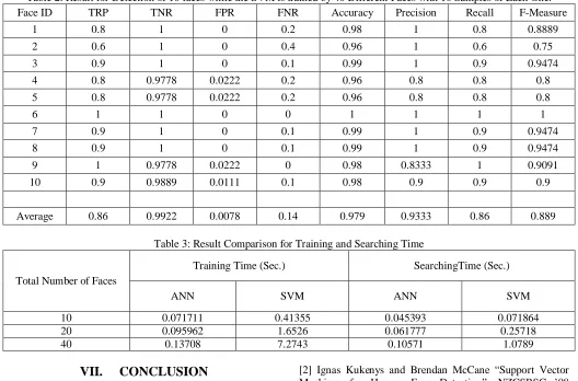
Figure 2: Sketch of determination of the number of boxes by the DBC method [11].

142

Copyright © 2017. Vandana Publications. All Rights Reserved.

Consider that the image of size 𝑀𝑀×𝑀𝑀 pixels has been scaled down to a size 𝑠𝑠×𝑠𝑠 where 𝑀𝑀

2 ≥ 𝑠𝑠> 1 and 𝑠𝑠 is an integer. Then we have an estimate of 𝑟𝑟= 𝑠𝑠/𝑀𝑀 . Now considering the image as a 3-D space with (𝑥𝑥,𝑦𝑦) denoting 2-D position and the third coordinate (𝑧𝑧) denoting gray level. The (𝑥𝑥,𝑦𝑦) space is partitioned into grids of size 𝑠𝑠×𝑠𝑠. Oneach grid there is a column of boxes of size 𝑠𝑠×𝑠𝑠 ×𝑠𝑠′. If the total number of gray levels is 𝐺𝐺then𝐺𝐺

𝑠𝑠′ =𝑀𝑀_𝑠𝑠 . For example,

see Fig. (2), where 𝑠𝑠=𝑠𝑠’ = 3. Assign numbers 1, 2, . .. to the boxes as shown. Let the minimum and maximum gray level of the image in the (𝑖𝑖,𝑗𝑗)𝑡𝑡ℎ grid fall in box number 𝑘𝑘 and 𝑙𝑙, respectively. The contribution of 𝑁𝑁_𝑟𝑟, in (𝑖𝑖,𝑗𝑗)𝑡𝑡ℎ grid.

𝑛𝑛𝑟𝑟(𝑖𝑖,𝑗𝑗) =𝑙𝑙 − 𝑘𝑘+ 1, … … … … . (2)

For example, in Fig. (3), 𝑛𝑛_𝑟𝑟(𝑖𝑖,𝑗𝑗) = 3−2 + 1. (Although in this figure, for simplicity, smooth image surface is taken, but in reality it will be digital image surface.) Because of the differential nature of computing𝑛𝑛_𝑟𝑟, it is named as the differential box-counting (DBC) approach. Taking contributions from all grids, we have

𝑁𝑁𝑟𝑟=� 𝑛𝑛𝑟𝑟(𝑖𝑖,𝑗𝑗) 𝑖𝑖,𝑗𝑗

, … … … . . (3)

𝑁𝑁𝑟𝑟, is counted for different values of 𝑟𝑟, i.e., different values

of 𝑠𝑠. Then using (1), we can estimate 𝐷𝐷, the fractal dimension, from the least square linear fit of 𝑙𝑙𝑜𝑜𝑙𝑙(𝑁𝑁_𝑟𝑟) against 𝑙𝑙𝑜𝑜𝑙𝑙(1/𝑟𝑟).

Next, we form a two dimensional matrix 𝐹𝐹𝐷𝐷_{𝑐𝑐𝑜𝑜𝑐𝑐𝑐𝑐}of size (𝑀𝑀×𝑀𝑀) ×𝑑𝑑.Thatis, 𝐹𝐹𝐷𝐷_{𝑐𝑐𝑜𝑜𝑐𝑐𝑐𝑐} = [𝑐𝑐₁,𝑐𝑐₂,𝑐𝑐₃, …𝑐𝑐_{𝑀𝑀×𝑀𝑀}], where each element𝑐𝑐_𝑖𝑖is a vector of size 𝑑𝑑 (total scales) with and each element in is related to the pixel at location (𝑖𝑖,𝑗𝑗). The final value of 𝐹𝐹𝐷𝐷_{𝑐𝑐𝑖𝑖𝑛𝑛𝑓𝑓𝑙𝑙} is computed as the fractal slope of the least square linearregression line by [9]:

𝐹𝐹𝐷𝐷𝑐𝑐𝑖𝑖𝑛𝑛𝑓𝑓𝑙𝑙(𝑖𝑖,𝑗𝑗) =𝑆𝑆𝑣𝑣(𝑖𝑖,_𝑆𝑆 𝑗𝑗)

𝑟𝑟 , … … … . . (4)

Where 𝑆𝑆_𝑟𝑟and 𝑆𝑆_𝑣𝑣are the sums of squares as follows:

𝑆𝑆𝑟𝑟= � (log(𝑟𝑟))2−�∑ log(𝑟𝑟) 𝑠𝑠𝑐𝑐𝑓𝑓𝑙𝑙𝑐𝑐 𝑠𝑠𝑡𝑡𝑜𝑜𝑡𝑡𝑓𝑓𝑙𝑙−1

𝑟𝑟=1 �

2

𝑠𝑠𝑐𝑐𝑓𝑓𝑙𝑙𝑐𝑐𝑠𝑠𝑡𝑡𝑜𝑜𝑡𝑡𝑓𝑓𝑙𝑙 −1 𝑠𝑠𝑐𝑐𝑓𝑓𝑙𝑙𝑐𝑐 𝑠𝑠𝑡𝑡𝑜𝑜𝑡𝑡𝑓𝑓𝑙𝑙 −1

𝑟𝑟=1

, … (5)

𝑆𝑆𝑣𝑣(𝑖𝑖,𝑗𝑗)

= � log(𝑟𝑟)�𝑐𝑐(𝑖𝑖,𝑗𝑗)�

𝑠𝑠𝑐𝑐𝑓𝑓𝑙𝑙𝑐𝑐 𝑠𝑠𝑡𝑡𝑜𝑜𝑡𝑡𝑓𝑓𝑙𝑙−1

𝑟𝑟=1

−�∑ log(𝑟𝑟)

𝑠𝑠𝑐𝑐𝑓𝑓𝑙𝑙𝑐𝑐 𝑠𝑠𝑡𝑡𝑜𝑜𝑡𝑡𝑓𝑓𝑙𝑙−1

𝑟𝑟=1 ��∑𝑠𝑠𝑐𝑐𝑓𝑓𝑙𝑙𝑐𝑐 𝑠𝑠𝑟𝑟=1 𝑡𝑡𝑜𝑜𝑡𝑡𝑓𝑓𝑙𝑙−1𝑐𝑐(𝑖𝑖,𝑗𝑗),𝑟𝑟�

𝑠𝑠𝑐𝑐𝑓𝑓𝑙𝑙𝑐𝑐𝑠𝑠𝑡𝑡𝑜𝑜𝑡𝑡𝑓𝑓𝑙𝑙 −1 , … (6)

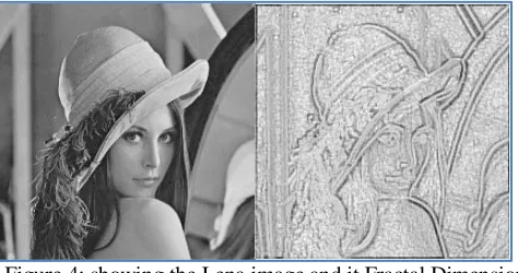
Figure 4: showing the Lena image and it Fractal Dimension Image.

The transformation process to convert face images to FD image as illustrated in Figure. 4.

IV.

SUPPORT VECTOR MACHINE (SVM)

Support Vector Machines (SVMs) have developed from Statistical Learning Theory [6]. They have been widely applied to fields such as character, handwriting digit and text recognition, and more recently to satellite image classification. SVMs, like ANN and other nonparametric classifiers have a reputation for being robust. SVMs function by nonlinearly projecting the training data in the input space to a feature space of higher dimension by use of a kernel function. This results in a linearly separable dataset that can be separated by a linear classifier. This process enables the classification of datasets which are usually nonlinearly separable in the input space. The functions used to project the data from input space to feature space are called kernels (or kernel machines), examples of which include polynomial, Gaussian (more commonly referred to as radial basis functions) and quadratic functions. By their nature SVMs are intrinsically binary classifiers however there are strategies by which they can be adapted to multiclass tasks. But in our case we not need multiclass classification.

4.1 SVM CLASSIFICATION

143

Copyright © 2017. Vandana Publications. All Rights Reserved.

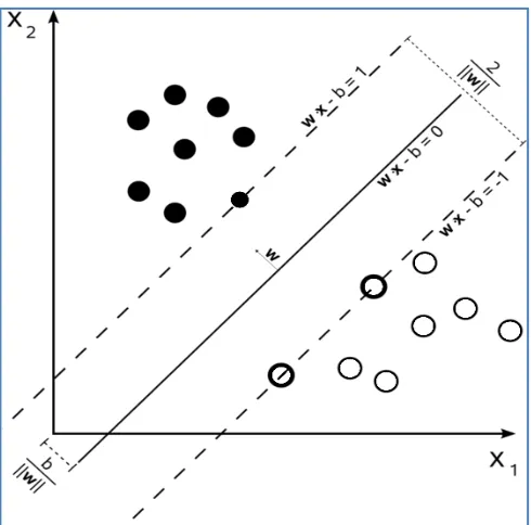
Figure 5: Maximum-margin hyper-plane and margins for an SVM trained with samples from two classes. Samples on the

margin (dashed line) are called the support vectors.

𝑦𝑦𝑖𝑖(〈𝑤𝑤.𝑥𝑥𝑖𝑖〉+𝑏𝑏)≥1,𝑖𝑖= 1 …𝑛𝑛, … . (7)

Where the hyper-plane is denoted by a vector of weights 𝒘𝒘and a bias term𝒃𝒃. The optimal separating hyper-plane, when classes have equal loss-functions, maximizes the margin between the hyper-plane and the closest samples of classes. The margin is given by

𝑑𝑑(𝑤𝑤,𝑏𝑏) = min_𝑥𝑥 𝑖𝑖,𝑦𝑦𝑖𝑖=1

|〈𝒘𝒘.𝑥𝑥𝑖𝑖〉+𝑏𝑏|

‖𝒘𝒘‖ + min𝑥𝑥𝑖𝑖,𝑦𝑦𝑖𝑖=−1

�〈𝒘𝒘.𝑥𝑥𝑗𝑗〉+𝑏𝑏�

‖𝒘𝒘‖ =_{‖𝒘𝒘‖}2 … … . . (8)

The optimal separating hyper-plane can now be solved by maximizing (8) subject to (7). The solution can be found using the method of Lagrange multipliers. The objective is now to minimize the Lagrangian

𝐿𝐿𝑝𝑝(𝑤𝑤,𝑏𝑏,𝑓𝑓) =1₂‖𝒘𝒘‖2− � 𝛼𝛼𝑖𝑖𝑦𝑦𝑖𝑖(〈𝒘𝒘.𝒙𝒙𝒊𝒊〉+𝑏𝑏) 𝑙𝑙

𝑖𝑖=1

+� 𝛼𝛼𝑖𝑖 𝑙𝑙

𝑖𝑖=1

… … … … . (9)

and requires that the partial derivatives of 𝒘𝒘and 𝒃𝒃be zero. In (9), 𝜶𝜶_𝒊𝒊is nonnegative Lagrange multipliers. Partial

derivatives propagate to constraints 𝑤𝑤=∑ 𝛼𝛼_{𝑖𝑖 𝑖𝑖}𝑦𝑦_𝑖𝑖𝑥𝑥_𝑖𝑖 𝑓𝑓𝑛𝑛𝑑𝑑 ∑ 𝛼𝛼_{𝑖𝑖 𝑖𝑖}𝑦𝑦_𝑖𝑖 = 0. Substituting

𝒘𝒘into (9) gives the dual form

𝐿𝐿𝑑𝑑(𝑤𝑤,𝑏𝑏,𝑓𝑓) =� 𝛼𝛼𝑖𝑖 𝑙𝑙

𝑖𝑖=1

−1₂� 𝛼𝛼𝑖𝑖𝛼𝛼𝑗𝑗𝑦𝑦𝑖𝑖 𝑙𝑙

𝑖𝑖,𝑗𝑗=1

𝑦𝑦𝑗𝑗〈𝑥𝑥𝑖𝑖.𝑥𝑥𝑗𝑗〉… . . (10)

Which is not anymore an explicit function of 𝒘𝒘or 𝒃𝒃. The optimal hyper-plane can be found by maximizing (10) subject to ∑ 𝛼𝛼_{𝑖𝑖 𝑖𝑖}𝑦𝑦_𝑖𝑖 = 0 and all Lagrange multipliers are nonnegative. However, in most real world situations classes are not linearly separable and it is not possible to find a linear hyper-plane that would satisfy (7) for all𝒊𝒊 = 𝟏𝟏. . .𝒏𝒏. In these cases a classification problem can be made linearly separable by using a nonlinear mapping into the feature space where classes are linearly separable. The condition for perfect classification can now be written as

𝑦𝑦𝑖𝑖�〈𝑤𝑤.∅�𝑥𝑥𝑗𝑗�〉+𝑏𝑏� ≥1,𝑖𝑖= 1, … . ,𝑛𝑛, … … (11)

Where𝜱𝜱 is the mapping into the feature space. Note that the feature mapping may change the dimension of the feature vector. The problem now is how to find a suitable mapping 𝜱𝜱 to the space where classes are linearly separable. It turns out that it is not required to know the mapping explicitly as can be seen by writing (11) in the dual form

𝑦𝑦𝑖𝑖�� 𝛼𝛼𝑖𝑖𝑦𝑦𝑖𝑖〈∅�𝑥𝑥𝑗𝑗�.∅(𝑥𝑥𝑖𝑖)〉 𝑙𝑙

𝑗𝑗=1

�+𝑏𝑏 ≥1,𝑖𝑖= 1, … ,𝑛𝑛… … . (12)

and replacing the inner product in (12) with a suitable kernel function 𝑘𝑘�𝑥𝑥_𝑗𝑗,𝑥𝑥_𝑖𝑖�=�∅�𝑥𝑥_𝑗𝑗�,∅(𝑥𝑥_𝑖𝑖)�. This form arises from the same procedure as was done in the linearly separable case that is, writing the Lagrangian of (12), solving partial derivatives, and substituting them back into the Lagrangian. Using a kernel trick, we can remove the explicit calculation of the mapping Φ and need to only solve the Lagrangian (11) in dual form, where the inner product �𝑥𝑥_𝑗𝑗,𝑥𝑥_𝑖𝑖�has been transposed with the kernel function in nonlinearly separable cases. In the solution of the Lagrangian, all data points with nonzero (and nonnegative) Lagrange multipliers are called support vectors (SV).

Often the hyper-plane that separates the training data perfectly would be very complex and would not generalize well to external data since data generally includes some noise and outliers. Therefore, we should allow some violation in (7) and (12). This is done with the nonnegative slack variable ζ

The slack variable is adjusted by the regularization constant C, which determines the tradeoff between complexity and the generalization properties of the classifier. This limits the Lagrange multipliers in the dual objective function (10) to the range 0 ≤ α

i

𝑦𝑦𝑖𝑖�〈𝑤𝑤.∅�𝑥𝑥𝑗𝑗�〉+𝑏𝑏� ≥1−,𝑖𝑖= 1, … . ,𝑛𝑛, … … (13)

144

Copyright © 2017. Vandana Publications. All Rights Reserved.

derived from mappings to the feature space satisfies the conditions for the kernel function.

The choice of a Kernel depends on the problem at hand because it depends on what we are trying to model. The SVM gives the following advantages over neural networks or other AI methods (link for more details http://www.svms.org).

SVM training always finds a global minimum, and their simple geometric interpretation provides fertile ground for further investigation.

Most often Gaussian kernels are used, when the resulted SVM corresponds to an RBF network with Gaussian radial basis functions. As the SVM approach “automatically” solves the network complexity problem, the size of the hidden layer is obtained as the result of the QP procedure. Hidden neurons and support vectors correspond to each other, so the center problems of the RBF network is also solved, as the support vectors serve as the basis function centers.

Classical learning systems like neural networks suffer from their theoretical weakness, e.g. back-propagation usually converges only to locally optimal solutions. Here SVMs can provide a significant improvement.

The absence of local minima from the above algorithms marks a major departure from traditional systems such as neural networks.

SVMs have been developed in the reverse order to the development of neural networks (NNs). SVMs evolved from the sound theory to the implementation and experiments, while the NNs followed more heuristic path, from applications and extensive experimentation to the theory.

V.

PROPOSED ALGORITHM

The proposed algorithm can be described in following steps.

1. Perform the log transformation on the original image. 2.Compute the 𝐹𝐹𝐷𝐷_{𝑐𝑐𝑜𝑜𝑐𝑐𝑐𝑐} matrix for 10 different scales or 𝑠𝑠𝑐𝑐𝑓𝑓𝑙𝑙𝑐𝑐𝑠𝑠_{𝑡𝑡𝑜𝑜𝑡𝑡𝑓𝑓𝑙𝑙} = 11 as presented in section 3.

3. Now compute the𝐹𝐹𝐷𝐷_{𝑡𝑡𝑜𝑜𝑡𝑡𝑓𝑓𝑙𝑙}from the 𝐹𝐹𝐷𝐷_{𝑐𝑐𝑜𝑜𝑐𝑐𝑐𝑐}as presented in section 3

4. Feature vectors are formed by forming the row matrix of coefficients of 𝐹𝐹𝐷𝐷_{𝑡𝑡𝑜𝑜𝑡𝑡𝑓𝑓𝑙𝑙} as follows:

𝐹𝐹𝐹𝐹(𝑖𝑖) =�𝐹𝐹𝐷𝐷𝑡𝑡𝑜𝑜𝑡𝑡𝑓𝑓𝑙𝑙(𝑖𝑖), 𝑖𝑖𝑐𝑐 𝐹𝐹𝐷𝐷𝑡𝑡𝑜𝑜𝑡𝑡𝑓𝑓𝑙𝑙(𝑖𝑖) >𝑡𝑡ℎ

0, 𝑜𝑜𝑡𝑡ℎ𝑐𝑐𝑟𝑟𝑤𝑤𝑖𝑖𝑠𝑠𝑐𝑐

5. These vectors are created for all classes of faces.

6. These vectors are used to train the 𝑁𝑁 ∗(𝑁𝑁 −1)/2 (𝑁𝑁 is the number of classes or different faces) SVM classifiers as we used one against one method.

7. For detection purpose the input image vectors are calculated in same way as during training and then it is applied on each classifier.

8. Finally the decision is mode on the basis of majority of class returned by N*(N-1)/2 classifiers.

VI.

SIMULATION RESULTS

We used the ORL database for testing of our algorithm. The ORL database contains 40 different faces with 10 samples of each face. The accuracy of the algorithm is tested for different number of faces, samples and vector length.

The comparison of the proposed method with Artificial Neural Network based method shows that the proposed method outperforms the ANN.

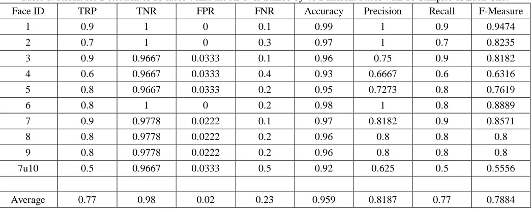
Table 1: Result for Detection of 10 faces while the ANN is trained by 40 Different Faces with 10 Samples of Each One.

Face ID TRP TNR FPR FNR Accuracy Precision Recall F-Measure

1 0.9 1 0 0.1 0.99 1 0.9 0.9474

2 0.7 1 0 0.3 0.97 1 0.7 0.8235

3 0.9 0.9667 0.0333 0.1 0.96 0.75 0.9 0.8182

4 0.6 0.9667 0.0333 0.4 0.93 0.6667 0.6 0.6316

5 0.8 0.9667 0.0333 0.2 0.95 0.7273 0.8 0.7619

6 0.8 1 0 0.2 0.98 1 0.8 0.8889

7 0.9 0.9778 0.0222 0.1 0.97 0.8182 0.9 0.8571

8 0.8 0.9778 0.0222 0.2 0.96 0.8 0.8 0.8

9 0.8 0.9778 0.0222 0.2 0.96 0.8 0.8 0.8

7u10 0.5 0.9667 0.0333 0.5 0.92 0.625 0.5 0.5556

145

Copyright © 2017. Vandana Publications. All Rights Reserved.

Table 2: Result for Detection of 10 faces while the SVM is trained by 40 Different Faces with 10 Samples of Each One.

Face ID TRP TNR FPR FNR Accuracy Precision Recall F-Measure

1 0.8 1 0 0.2 0.98 1 0.8 0.8889

2 0.6 1 0 0.4 0.96 1 0.6 0.75

3 0.9 1 0 0.1 0.99 1 0.9 0.9474

4 0.8 0.9778 0.0222 0.2 0.96 0.8 0.8 0.8

5 0.8 0.9778 0.0222 0.2 0.96 0.8 0.8 0.8

6 1 1 0 0 1 1 1 1

7 0.9 1 0 0.1 0.99 1 0.9 0.9474

8 0.9 1 0 0.1 0.99 1 0.9 0.9474

9 1 0.9778 0.0222 0 0.98 0.8333 1 0.9091

10 0.9 0.9889 0.0111 0.1 0.98 0.9 0.9 0.9

Average 0.86 0.9922 0.0078 0.14 0.979 0.9333 0.86 0.889

Table 3: Result Comparison for Training and Searching Time

Total Number of Faces

Training Time (Sec.) SearchingTime (Sec.)

ANN SVM ANN SVM

10 0.071711 0.41355 0.045393 0.071864

20 0.095962 1.6526 0.061777 0.25718

40 0.13708 7.2743 0.10571 1.0789

VII. CONCLUSION

This paper presents a Fractal Dimension based feature extraction approach in combination with Support Vector Machine (SVM) for the classification phase, the results are also compared with Artificial Neural Network (ANN)classifier. For the detailed analysis wide facial variations has been considered by taking the ORL database for the conducted experiments. The experimental results indicate that the fractal dimensions provides a good method for feature extraction for face recognition system as the results shows the average accuracy up to 97.4%. Considering the comparison between the SVM and NN the results reveals that the SVM method performs better than ANN when compared for recognition accuracy but when compared for training and detection time the neural network out performs the SVM. However the SVM presently tested with only linear kernel function hence the results can be further improved by using different kernel functions such as Quadratic, Polynomial, and RBF etc. we presently leave this work for future implementations.

REFERENCES

[1] "Biometrics: Overview", Biometrics.cse.msu.edu. 6 September 2007. Retrieved 2012-06-10

[2] Ignas Kukenys and Brendan McCane “Support Vector Machines for Human Face Detection”, NZCSRSC ’08 Christchurch New Zealand.

[3] Jixiong Wang (jameswang) “CSCI 1950F Face Recognition Using Support Vector Machine: Report”, Spring 2011, May 24, 2011.

[4] Antony Lam & Christian R. Shelton “Face Recognition and Alignment using Support Vector Machines”, 2008 IE. [5] Jennifer Huang, Volker Blanz and Bernd Heisele “Face Recognition Using Component-Based SVM Classification and Morphable Models”, SVM 2002, LNCS 2388, pp. 334– 341, 2002. Springer-Verlag Berlin Heidelberg 2002.

[6] Bernd Heisele, Purdy Ho and Tomaso Poggio “Face Recognition with Support Vector Machines: Global versus Component-based Approach”, Massachusetts Institute of Technology Center for Biological and Computational Learning Cambridge, MA 02142.

[7] Yongmin Li, Shaogang Gong, Jamie Sherrah and Heather Liddell “Support vector machine based multi-view face detection and recognition”, Image and Vision Computing 22 (2004) 413–427.

[8] Qiong Wang, Jingyu Yang, and Wankou Yang “Face Detection using Rectangle Features and SVM”, International Journal of Electrical and Computer Engineering 1:7 2006.

.

146

Copyright © 2017. Vandana Publications. All Rights Reserved.

Fractal Analysis”, IEEE Signal Processing Letters, Vol. 21, No. 12, December 2014.

[10] Nirupam Sarkar and B. B. Chaudhuri “An Efficient Differential Box-Counting Approach to Compute Fractal Dimension of Image”, IEEE Transactions On Systems, Man, And Cybernetics, Vol. 24, No. I. January 1994. [11] Jian Li, Qian Du, Caixin Sun “An improved box-counting method for image fractal dimension estimation”, Pattern Recognition Volume 42, Issue 11, November 2009, Pages 2460–2469.