An Easy-to-hard Learning Paradigm for Multiple Classes
and Multiple Labels
Weiwei Liu [email protected]
School of Computer Science and Engineering The University of New South Wales, Sydney NSW 2052, Australia
and
Centre for Artificial Intelligence FEIT, University of Technology Sydney NSW 2007, Australia
Ivor W. Tsang [email protected]
Centre for Artificial Intelligence FEIT, University of Technology Sydney NSW 2007, Australia
Klaus-Robert M¨uller [email protected]
Machine Learning Group, Computer Science Berlin Institute of Technology (TU Berlin) Marchstr 23, 10587 Berlin, Germany and
Max Planck Institute for Informatics Stuhlsatzenhausweg, 66123, Saarbrcken and
Department of Brain and Cognitive Engineering Korea University, Seoul 02841, Korea
Editor:Karsten Borgwardt
Abstract
Many applications, such as human action recognition and object detection, can be formu-lated as a multiclass classification problem. One-vs-rest (OVR) is one of the most widely used approaches for multiclass classification due to its simplicity and excellent performance. However, many confusing classes in such applications will degrade its results. For example,
hand clapandboxingare two confusing actions. Hand clapis easily misclassified asboxing, and vice versa. Therefore, precisely classifying confusing classes remains a challenging task. To obtain better performance for multiclass classifications that have confusing classes, we first develop a classifier chain model for multiclass classification (CCMC) to transfer class information between classifiers. Then, based on an analysis of our proposed model, we propose an easy-to-hard learning paradigm for multiclass classification to automatically identify easy and hard classes and then use the predictions from simpler classes to help solve harder classes. Similar to CCMC, the classifier chain (CC) model is also proposed by Read et al. (2009) to capture the label dependency for multi-label classification. How-ever, CC does not consider the order of difficulty of the labels and achieves degenerated performance when there are many confusing labels. Therefore, it is non-trivial to learn the
c
appropriate label order for CC. Motivated by our analysis for CCMC, we also propose the easy-to-hard learning paradigm for multi-label classification to automatically identify easy and hard labels, and then use the predictions from simpler labels to help solve harder la-bels. We also demonstrate that our proposed strategy can be successfully applied to a wide range of applications, such as ordinal classification and relationship prediction. Extensive empirical studies validate our analysis and the effectiveness of our proposed easy-to-hard learning strategies.
Keywords: Multiclass Classification, Multi-label Classification, Classifier Chain, Easy-to-hard Learning Paradigm
1. Introduction
Many applications can be formulated as a multiclass classification problem. For example, human action recognition aims to classify videos into different categories of human action. In the KTH data set (Sch¨uldt et al., 2004), for example, there are six types of human action:
walk, jog, run, hand wave,hand clap and boxing. These actions can be classified into two main categories: leg movements (walk,jog andrun) and hand movements (hand wave,hand clap andboxing). It is easy to differentiate between leg and hand movements, such aswalk
and hand wave, but actions within leg or hand movements, such as hand clap and boxing, are easily confused. Hand clap is easily misclassified as boxing, and vice versa. Confusing classes are ubiquitous in real world applications, especially for data sets with many classes. For example, there are many confusing classes in the ALOI data set from the LIBSVM website1, which contains 1,000 classes. Therefore, precisely classifying multiclass data sets with confusing classes is a challenging task.
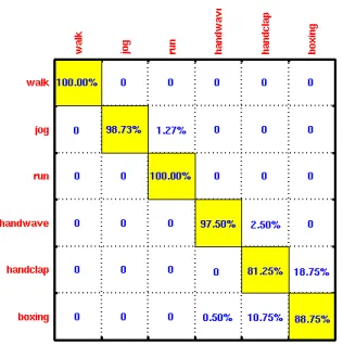
From the confusion matrix of one-vs-rest (OVR) on the KTH data set shown in Figure 1, we observe thatwalk is the easiest action to classify and hand clap is the hardest action to classify, as the walk action can be correctly identified by OVR whereas the percentage of
hand clap images that are misclassified as boxing is 22.5%. To achieve accurate prediction performance, according to Figure 1, we should classify walk first, followed by run,jog and
hand wave. Boxing andhand clapare the last two actions to classify. The motivation behind this paper is to solve classification tasks from easy to hard, and to use the predictions from simpler tasks to help solve the harder tasks.
To achieve our goal, a classifier chain model for multiclass classification (CCMC) is pro-posed to transfer class information between classifiers. Furthermore, we generalize CCMC over a random class order and provide a theoretical analysis of the generalization error for the proposed generalized model. Our results show that the upper bound of the general-ization error depends on the sum of the reciprocal of the square of the margin over the classes. Therefore, we conclude that class order does affect the performance of CCMC, and a globally optimal class order exists only when the minimization of the upper bound is achieved over this CCMC. Lastly, based on our results, we propose the easy-to-hard learning paradigm for multiclass classification to automatically identify easy and hard classes and then use the predictions from simpler classes to help solve harder classes.
Multi-label classification, where each instance can belong to multiple labels simultane-ously, has garnered significant attention from researchers as a result of its various
Figure 1: Confusion Matrix of OVR on the KTH Data Set. In the confusion matrix, the entry in the i-th row and j-th column is the percentage of images from action i that are misclassified as action j. Average classification accuracy rates for individual actions are listed along the diagonal, which is colored yellow.
tions, which range from document classification and gene function prediction, to automatic image annotation. For example, a document can be associated with a range of topics, such asSports,Finance and Education (Schapire and Singer, 2000); a gene belongs to the functions ofprotein synthesis,metabolism and transcription (Barutcuoglu et al., 2006); an image may have bothbeach and tree tags (Boutell et al., 2004).
Similar to CCMC, a classifier chain (CC) model is also proposed by Read et al. (2009) to capture the label dependency for multi-label classification. It also tries to use information from previous labels to help train the classifier for the next label. However, CC’s perfor-mance degenerates when there are many confusing labels, because the main drawback of CC is that it does not consider the order of difficulty of the labels. Therefore, it is non-trivial to learn the appropriate label order for CC.
Motivated by our analysis for CCMC, we first generalize CC over a random label order and provide the generalization error bound for the proposed generalized model. Then we propose the easy-to-hard learning paradigm for multi-label classification to automatically identify easy and hard labels. Lastly, we use the predictions from simpler labels to help solve harder labels. To learn the objective of our proposed easy-to-hard learning paradigms, it is very expensive to search overq! different class or label orders2, whereq denotes the number of classes or labels, which is computationally infeasible for a largeq. We thus propose a set of easy-to-hard learning algorithms to simplify the search process of the optimal learning sequence.
Experiments on a wide spectrum of data sets show that our proposed methods excel in all data sets for multi-label and multiclass classification problems. The results validate our analysis and the effectiveness of our proposed easy-to-hard learning algorithms. Lastly, we demonstrate that our proposed easy-to-hard learning strategies can be successfully applied
to a wide range of applications, such as ordinal classification (Chu and Ghahramani, 2005) and relationship prediction (Massa and Avesani, 2006).
We organize this paper as follows. Section 2 summarizes existing related works and problems. The easy-to-hard learning paradigm for multi-label and multiclass classification are proposed in Sections 3 and 4. Learning algorithms and time complexity analysis are described in Section 5. We present two applications in Section 6. Section 7 shows the comprehensive experimental results. The last section provides concluding remarks.
Notations: Assumext∈Rdis a real vector representing an input or instance (feature)
fort∈ {1,· · · , n}. ndenotes the number of training instances. Yt⊆ {λ1, λ2,· · ·, λq}is the
corresponding output (class or label). yt ∈ {0,1}q is used to represent the set Y
t, where
yt(j) = 1 if and only ifλj ∈ Yt. Note that, there is only one element inYtfor the multiclass
problem.
2. Related Work and Problems
2.1 Multiclass Classification
2.1.1 OVR and OVO
One-vs-rest (OVR) and one-vs-one (OVO) are two famous strategies for decomposing mul-ticlass classification problems into multiple binary classification problems. Hsu and Lin (2002), Rifkin and Klautau (2004), Demirkesen and Cherifi (2008) and Lapin et al. (2015, 2016) have already shown that OVR and OVO are successful schemes that are as accurate as more complicated approaches, such as error-correcting output coding (ECOC) (Dietterich and Bakiri, 1995), the tree-based method (Beygelzimer et al., 2009a,b; Bengio et al., 2010; Yang and Tsang, 2011; Liu and Tsang, 2016) and multi-class SVM (Weston and Watkins, 1999; Lapin et al., 2015, 2016).
OVR works as follows: a binary classifier is trained for each class λj, with all of the
instances in the j-th class having positive labels, and all other instances having negative labels. q binary classifiers are then trained on {xt,yt(1)}nt=1,· · ·,{xt,yt(q)}nt=1. The final output of OVR for each testing instance is the class that corresponds to the classifier with the highest output value. OVR ignores correlations between classes and each classifier is trained independently. OVO trains all possibleq(q−1)/2 binary classifiers from a training set ofq classes, where each classifier is trained on only two out ofq classes.
2.1.2 Rifkin and Klautau’s conjecture
OVR is a lower cost approach with many more applications than OVO. However, Rifkin and Klautau (2004), who conduct a thorough study on OVR, point out that the condition of OVR working as well as any other clever schemes is that the classes are independent - we do not necessarily expect instances from class “A” to be closer to those in class “B” than those in class “C”. They also speculate that an algorithm that exploits the relationship between classes could offer superior performance, and that this would remains an open problem. To the best of our knowledge, this problem has still not been well-addressed, which is why the present paper studies this problem to provide an answer.
2.2 Multi-label Classification
One popular strategy for multi-label classification is to reduce the original problem into many binary classification problems. Many works have followed this strategy. For example, binary relevance (BR) (Tsoumakas et al., 2010) is a simple approach for multi-label learning which independently trains a binary classifier for each label. Recently, Chen and Lin (2012); Liu and Tsang (2015a,b); Zhang and Zhou (2014); Gong et al. (2017); Liu and Tsang (2017) have shown that multi-label learning methods that explicitly capture label dependency will usually achieve better prediction performance. Therefore, modeling label dependency is one of the major challenges in multi-label classification problems.
To capture label dependency, Hsu et al. (2009) first use the compressed sensing technique to handle multi-label classification problems. They project the original label space into a low dimensional label space. A regression model is then trained on each transformed label. Lastly, multi-labels are recovered from the regression output, which usually involves solving a quadratic programming problem (Hsu et al., 2009). Many works have been developed in this way (Zhang and Schneider, 2011, 2012; Tai and Lin, 2012). Such methods mainly aim to use different projection methods to transform the original label space into another effective label space. However, an expensive encoding and decoding procedure prevents these methods from being practical.
Another important approach attempts to exploit the different orders (first-order, second-order and high-second-order) of label correlations (Zhang and Zhang, 2010; Zhang and Zhou, 2014). Following this way, some works try to provide a probabilistic interpretation for label corre-lations. For example, Guo and Gu (2011) model the label correlations using a conditional dependency network; PCC (Dembczynski et al., 2010) exploits a high-order Markov Chain model to capture the correlations between the labels and provide an accurate probabilistic interpretation of classifier chain (CC) (Read et al., 2009). Some other works (Kang et al., 2006; Read et al., 2009; Huang and Zhou, 2012) focus on modeling the label correlations in a deterministic way. Among them, the CC model is one of the most popular methods due to its simplicity and promising experimental results (Read et al., 2009).
because different classifier chains involve different classifiers trained on different training sets. Thus, to reduce the influence of the label order, Read et al. (2009) propose the ensemble of classifier chains (ECC) to average the multi-label predictions of CC over a set of random ordering chains. Since the performance of CC is sensitive to the choice of label, there is another important question: Is there any globally optimal classifier chain which can achieve the optimal prediction performance for CC? If yes, how can the globally optimal classifier chain be found? This paper studies this problem and provides an answer.
2.3 Curriculum Learning
Curriculum learning (Bengio et al., 2009) can be seen as a sequence of training criteria. Each training criterion in the sequence is associated with a different set of weights in the training examples, or more generally, in a re-weighting of the training distribution. Initially, the weights favor easier examples that can be learned most easily. The next training crite-rion involves a slight change in the weighting of examples that increases the probability of sampling slightly more difficult examples. Overall, curriculum learning aims to find easier examples. However, up to now, curriculum learning has not defined what easy examples mean, or equivalently, how to sort the examples into a sequence that illustrates the simpler concepts first.
Inspired by curriculum learning, this paper clearly defines easy and hard tasks and provides the strategy to learn easy and hard tasks. Our empirical studies verify that our method is able to automatically identify easy and hard tasks, and use the predictions of classifiers from easier tasks to train the classifier for harder tasks.
3. The Easy-to-hard Learning Paradigm for Multiclass Classification
3.1 Classifier Chain for Multiclass Classification
In multi-label classification, each instance can belong to multiple labels simultaneously, while multiclass classification classifies instances into one of more than two classes. There-fore, multiclass classification (Hsu and Lin, 2002) is a quite different learning task compared to multi-label classification (Zhang and Zhou, 2014). Many applications, such as human action recognition and object detection, can be formulated as a multiclass classification problem. However, many confusing classes in such applications will degrade the existing solver’s performance. For example, hand clap and boxing are two confusing actions. Hand clap is easily misclassified as boxing, and vice versa. Therefore, it is non-trivial to precisely classify confusing classes for multiclass classification.
To solve these issues, motivated by CC for multi-label classification, we propose a clas-sifier chain model for multiclass classification (CCMC) which aims to transfer class infor-mation between classifiers. CCMC trainsqbinary classifiershj (j∈ {1,· · ·, q}), with all of
the instances in thej-th class having positive labels, and all other instances having negative labels. Similar to CC, classifiers of CCMC are linked along a chain. CCMC works as follows: binary classifier h1 is first trained for class λ1, then the augmented vector {xt, h1(xt)}nt=1 is used as the input to train classifier h2 for class λ2. Similarly, xt augments all previous
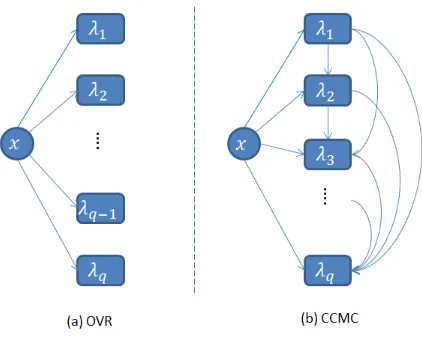
Figure 2: Schematic illustration of OVR and CCMC. A circle represents the input x. A rectangle represents class λi(t ∈ {1,· · · , q}). The starting point of the arrow
denotes the input to train the classifier for the class to which the arrow points.
Given a new testing instancex, classifierh1 in the chain is responsible for predicting the value for λ1 using input x. h2 predicts the value for λ2 taking x plus the predicted value of h1(x) as an input. Similarly, hj+1 predicts the value for λj+1 using x plus all previous prediction results fromh1,· · · , hj as the input. CCMC proceeds in this way until the value
of the last classλq has been predicted. Similar to OVR, the final output of CCMC for xis
the class that corresponds to the classifier with the highest output value. CCMC exploits the class dependence by passing class information between classifiers. Figure 2 illustrates the working scheme between OVR and CCMC.
3.2 Generalized Classifier Chain for Multiclass Classification
We generalize the CCMC model over a random class order, calledgeneralized classifier chain for multiclass classification (GCCMC). Assume that classes {λ1, λ2,· · ·, λq} are randomly
reordered as{ζ1, ζ2,· · ·, ζq}, whereζj =λk means class λk moves to position j fromk. In
the GCCMC model, classifiers are also linked along a chain where each classifier hj deals
with the binary classification problem for classζj (λk). GCCMC follows the same training
and testing procedures as CCMC, the only difference being the class order.
3.3 Analysis
Let X represent the input space. Both s and ¯s are m multiclass examples drawn inde-pendently according to an unknown distributionD. We denote logarithms to base 2 by log. IfS is a set,|S| denotes its cardinality. k · kmeans the l2 norm.
We begin with the definition of the fat shattering dimension.
Definition 1 (Kearns and Schapire (1990)) Let H be a set of real valued functions.
We say that a set of points P is γ-shattered by H relative to r = (rp)p∈P if there are real numbers rp indexed by p ∈ P such that for all binary vectors b indexed by P, there is a functionfb ∈ H satisfying
fb(p) = (
≥rp+γ if bp= 1
≤rp−γ otherwise
The fat shattering dimensionf at(γ)of the setHis a function from the positive real numbers to the integers which maps a valueγ to the size of the largestγ-shattered set, if this is finite, or infinity otherwise.
Assume that H is the real valued function class andh ∈ H. l(y, h(x)) denotes the loss function. The expected error of h is defined as erD[h] = E(x,y)∼D[l(y, h(x))], where (x, y)
drawn from the unknown distribution D. Here we select 0-1 loss function. So, erD[h] =
P(x,y)∼D(h(x)6=y). The empirical risk ers[h] is defined as ers[h] = 1n
n P
t=1
I yt6=h(xt)
.3 Suppose that N(,H,s) is the -covering number of H with respect to the l∞
pseudo-metric measuring the maximum discrepancy on the examples. The notion of the covering number can be referred to Appendix A. We introduce the following general corollary re-garding the bound of the covering number:
Corollary 2 (Shawe-Taylor et al. (1998)) LetHbe a class of functionsX→[a, b]and
D a distribution over X. Choose0< <1 and let d=f at(/4)≤em. Then
E(N(,H,s))≤2
4m(b−a)2
2
dlog(2em(b−a)/(d))
(1)
where the expectation E is over examples s∈Xm drawn according toDm.
We study the generalization error bound of the specified GCCMC with the speci-fied number of classes and margins. Let G be the set of classifiers of GCCMC, G = {h1, h2,· · ·, hq}. ers[G] denotes the fraction of the number of errors that GCCMC makes
on s. Define ˆx∈X× {0,1}, ˆhj(ˆx) =hj(x)(1−y(j))−hj(x)y(j).
We introduce the following proposition:
Proposition 3 If an instance x ∈ X is misclassified by a GCCMC model, then ∃hj ∈
G,ˆhj(ˆx)≥0.
Proof For multiclass problem, assume that an instance x belongs to class ζi: y(i) = 1,
y(g) = 0(∀g∈ {1,2,· · · , q}, g6=i), and that it is misclassified asζj. Suppose that classifier
hj ∈Greports the highest confidence score for this instance: hj(x).
3. The expressionI yt6=h(xt)
Case 1: hj(x)≥0. In this case, ˆhj(ˆx) =hj(x)(1−y(j))−hj(x)y(j) =hj(x)≥0.
Case 2: hj(xt) < 0. In this case, all classifiers will output negative real numbers as
the result of hj reporting the highest confidence score. Thus, ˆhi(ˆx) = hi(x)(1−y(i))−
hi(x)y(i) =−hi(x)≥0.
Lemma 4 Given a specified GCCMC model with q classes and with marginsγ1, γ2,· · ·, γq
for each class satisfyingki=f at(γi/8), wheref at is continuous from the right. If GCCMC has correctly classified m multiclass examples s generated independently according to the unknown (but fixed) distribution D and ¯s is a set of another m multiclass examples, then we can bound the following probability to be less than δ: P2m{s¯s : ∃ a GCCMC model, it correctly classifies s, fraction of ¯s misclassified > (m, q, δ)} < δ, where (m, q, δ) =
1
m(Qlog(32m) + log
2q
δ) andQ= Pq
i=1kilog(8emki ).
Proof (of Lemma 4). Suppose thatGis a GCCMC model withq classes and with margins
γ1, γ2,· · ·, γq, the probability event in Lemma 4 can be described as
A={s¯s:∃G, ki=f at(γi/8), ers[G] = 0, er¯s[G]> }.
Let ˆsand ˆ¯sdenote two different set ofmmulticlass examples, which are drawn i.i.d. from the distributionD×{0,1}. Applying the definition ofˆx, ˆhand Proposition 3, the event can also be written as A = {ˆsˆ¯s : ∃G,γˆi = γi/2, ki =f at(ˆγi/4), ers[G] = 0, ri =maxtˆhi(ˆxt),2ˆγi =
−ri,|{yˆ ∈ ˆ¯s : ∃hi ∈ G,ˆhi(yˆ) ≥ 2ˆγi +ri}| > m}. Here, −maxtˆhi(ˆxt) means the minimal
value of |hi(x)| which represents the margin for class ζi, so 2ˆγi =−ri. Letγki =min{γ
0 :
f at(γ0/4)≤ki}, soγki ≤γˆ
i, we define the following function:
π(ˆh) =
0 if ˆh≥0 −2γki if ˆh≤ −2γki ˆ
h otherwise
soπ(ˆh)∈[−2γki,0]. Let π( ˆG) ={π(ˆh) :h∈G}. Let Bki
ˆ
sˆ¯s represent the minimalγki-cover set ofπ( ˆG) in the pseudo-metric dˆsˆ¯s. We have
that for any hi ∈ G, there exists ˜f ∈ Bˆksˆ¯si, |π(ˆhi(zˆ))−π( ˜f(ˆz))| < γki, for all ˆz ∈ ˆsˆ¯s. For all ˆx ∈ ˆs, by the definition of ri, ˆhi(ˆx) ≤ ri = −2ˆγi, and γki ≤ ˆγ
i, ˆh
i(ˆx) ≤ −2γki,
π(ˆhi(ˆx)) =−2γki, soπ( ˜f(xˆ))<−2γki +γki =−γki. However, there are at leastmpoints
ˆ
y ∈ˆ¯s such that ˆhi(ˆy) ≥0, so π( ˜f(yˆ))> −γki > maxtπ( ˜f(xˆt)). Since π only reduces the separation between output values, we conclude that the inequality ˜f(ˆy)> maxtf˜(ˆxt) holds.
Moreover, the m points in ˆ¯s with the largest ˜f values must remain for the inequality to hold. By the permutation argument, at most 2−m of the sequences obtained by swapping corresponding points satisfy the conditions for fixed ˜f.
As for any hi ∈G, there exists ˜f ∈Bˆks¯sˆi, so there are|Bˆskˆ¯si|possibilities of ˜f that satisfy
the inequality for ki. Note that |Bˆskˆ¯si| is a positive integer which is usually bigger than 1,
and by the union bound, we obtain the following inequality:
Since every set of points γ-shattered by π( ˆG) can be γ-shattered by ˆG, so f atπ( ˆG)(γ) ≤ f atGˆ(γ), where ˆG={ˆh:h∈G}. Hence, by Corollary 2 (setting [a, b] to [−2γki,0], toγki and m to 2m),
E(|Bki ˆ
sˆ¯s|) =E(N(γki, π( ˆG),ˆsˆ¯s))≤2(32m)
dlog(8emd ) where d= f atπ( ˆG)(γki/4) ≤f atGˆ(γki/4)≤ ki. Thus E(|B
ki
ˆsˆ¯s|) ≤ 2(32m)
kilog(8emki )
, and we obtain
P(A)≤(E(|Bsˆk1ˆ¯s|)× · · · ×E(|Bkq ˆsˆ¯s|))2
−m ≤
q Y
i=1
2(32m)kilog(8kiem)
= 2q(32m)Q
whereQ=Pqi=1kilog(8kemi ). And so (E(|Bˆsk1sˆ¯|)× · · · ×E(|Bsˆkˆ¯sq|))2−m< δ provided
(m, q, δ)≥ 1 m
Qlog(32m) + log2
q
δ
as required.
Lemma 4 applies to a particular GCCMC model with a specified number of classes and a specified margin for each class. In practice, we will observe the margins after running the GCCMC model. Thus, we must bound the probabilities uniformly over all of the possible margins to obtain a practical bound. The generalization error bound of the multiclass classification problem using GCCMC is shown as follows:
Theorem 5 Suppose that random m multiclass examples can be correctly classified using a GCCMC model, and suppose this GCCMC model contains q classifiers with margins
γ1, γ2,· · ·, γq for each class. Then we can bound the generalization error with probability greater than 1−δ to be less than
130R2 m
Q0log(8em) log(32m) + log2(2m)
q
δ
whereQ0=Pqi=1 (γ1i)2 andRis the radius of a ball containing the support of the distribution.
Before proving Theorem 5, we state one key symmetrization lemma and Theorem 7.
Lemma 6 (Symmetrization) Let H be the real valued function class. s and ¯s are m
examples both drawn independently according to the unknown distribution D. If m2 ≥ 2, then
Ps(sup h∈H
|erD[h]−ers[h]| ≥) ≤ 2Ps¯s(sup h∈H
|er¯s[h]−ers[h]| ≥/2) (2) The proof of this lemma can be found in Appendix B.
Theorem 7 (Bartlett and Shawe-Taylor (1998)) Let H be restricted to points in a
ball of M dimensions of radiusR about the origin, then
f atH(γ)≤min nR2
γ2,M+ 1
o
Proof (of Theorem 5). We must bound the probabilities over different margins. We first use Lemma 6 to bound the probability of error in terms of the probability of the discrepancy between the performance on two halves of a double example. Then we combine this result with Lemma 4. We must consider all possible patterns of ki’s for ζi. The largest value of
ki is m. Thus, for fixed q, we can bound the number of possibilities by mq. Hence, there
aremq of applications of Lemma 4.
Let ci={γ1, γ2,· · · , γq} denote thei-th combination of margins varied in{1,· · · , m}q.
G denotes a set of GCCMC models. The generalization error of G can be represented as
erD[G] anders[G] is 0, whereG∈ G. The uniform convergence bound of the generalization
error is
Ps(sup
G∈G
|erD[G]−ers[G]| ≥)
Applying Lemma 6,
Ps(sup
G∈G
|erD[G]−ers[G]| ≥)≤2Ps¯s(sup
G∈G
|er¯s[G]−ers[G]| ≥/2)
LetJci ={s¯s:∃a GCCMC modelGwithqclasses and with marginsci:ki =f at(γ
i/8), er
s[G] =
0, er¯s[G]≥/2}. Clearly,
Ps¯s(sup
G∈G
|er¯s[G]−ers[G]| ≥/2)≤Pm
qm
q
[
i=1 Jci
As ki still satisfies ki =f at(γi/8), Lemma 4 can still be applied to each case of Pm
q (Jci). Letδk=δ/mq. Applying Lemma 4 (replacing δ by δk/2), we get:
Pmq(Jci)< δk/2
where (m, k, δk/2) ≥ 2/m(Qlog(32m) + log2×2
q
δk ) and Q =
Pq
i=1kilog(4kemi ). It suffices
to show by the union bound that Pmq(Smi=1q Jci) ≤
Pmq
i=1Pm q
(Jci) < δk/2×m
q = δ/2.
Applying Lemma 6,
Ps(sup
G∈G
|erD[G]−ers[G]| ≥)≤2Ps¯s(sup
G∈G
|er¯s[G]−ers[G]| ≥/2)
≤2Pmq
m
q
[
i=1 Jci
< δ
Thus, Ps(supG∈G|erD[G]−ers[G]| ≤ ) ≥1−δ. Let R be the radius of a ball containing
the support of the distribution. Applying Theorem 7, we getki =f at(γi/8)≤65R2/(γi)2.
Note that we have replaced the constant 82 = 64 by 65 in order to ensure the continuity from the right required for the application of Lemma 4. We have upperbounded log(8em/ki)
by log(8em). Thus,
erD[G]≤2/m
Qlog(32m) + log2(2m)
q
δ
≤ 130R 2 m
Q0log(8em) log(32m) + log2(2m)
q
δ
whereQ0 =Pqi=1(γ1i)2.
Given the training data size and the number of classes, Theorem 5 reveals an important factor in reducing the generalization error bound for the GCCMC model: the minimization of the sum of the reciprocal of the square of the margin over the classes. Thus, we obtain the following Corollary:
Corollary 8 (Globally Optimal Classifier Chain for Multiclass Classification) Suppose
that random m multiclass examples with q classes can be correctly classified using a GC-CMC model, this GCGC-CMC model is the globally optimal classifier chain if and only if the minimization of Q0 in Theorem 5 is achieved over this classifier chain.
Based on Corollary 8, we propose the following easy-to-hard learning paradigm for multiclass classification problems.
Definition 9 (Easy-to-hard Learning Paradigm for Multiclass Classification) The
easy-to-hard learning paradigm for multiclass classification problem is to minimize Q0 in Theorem 5. By minimizingQ0, we can automatically identify easy and hard classes.
Remark. Classes with a larger margin are easier to identify than those with a smaller margin. Thus, the intuitive idea of the easy-to-hard learning paradigm is to identify the class with a larger margin first, followed by ones with a smaller margin.
Discussion of Rifkin and Klautau’s Conjecture. Rifkin and Klautau (2004)
spec-ulate that an algorithm which exploits the relationship between classes can offer superior performance, and this remains an open problem. Theoretically, Corollary 10 provides an affirmative answer to Rifkin and Klautau (2004)’s conjecture based on Theorem 5:
Corollary 10 By exploiting the relationship between classes, our proposed GCCMC model is able to achieve a lower generalization error bound. Furthermore, our proposed easy-to-hard learning paradigm can optimize the performance of GCCMC.
Motivated by the above analysis, we derive the following easy-to-hard learning paradigm for multi-label classification.
4. The Easy-to-hard Learning Paradigm for Multi-label Classification
4.1 Classifier Chain for Multi-label Classification
Similar to CCMC, theclassifier chain(CC) model (Read et al., 2009) is proposed to trainq
binary classifiershj (j∈ {1,· · ·, q}) for multi-label problems. Classifiers are linked along a
chain where each classifierhj deals with the binary classification problem for labelλj. The
Different classifier chains involve different classifiers learned on different training sets and thus the order of the chain itself clearly affects the prediction performance. To solve the issue of selecting a chain order for CC, Read et al. (2009) propose the extension of CC, called ensembled classifier chain (ECC), to average the multi-label predictions of CC over a set of random chain ordering. ECC first randomly reorders the labels {λ1, λ2,· · ·, λq}
many times. Then, CC is applied to the reordered labels for each time and the performance of CC is averaged over those times to obtain the final prediction performance.
4.2 Generalized Classifier Chain for Multi-label Classification
We generalize the CC model over a random label order, called generalized classifier chain
(GCC) model. Assume the labels{λ1, λ2,· · ·, λq}are randomly reordered as{ζ1, ζ2,· · · , ζq},
where ζj =λk means label λk moves to position j from k. In the GCC model, classifiers
are also linked along a chain where each classifier hj deals with the binary classification
problem for label ζj (λk). GCC follows the same training and testing procedures as CC,
while the only difference is the label order. In the GCC model, for input xt, yt(j) = 1 if
and only if ζj ∈ Yt.
4.3 Analysis
Motivated by our analysis in Section 3, we analyze the generalization error bound of the multi-label classification problem using GCC.
Let X represent the input space. Both s and ¯s are m multi-label examples drawn independently according to an unknown distribution D.
We first study the generalization error bound of the specified GCC with the specified number of labels and margins. LetGbe the set of classifiers of GCC,G={h1, h2,· · · , hq}.
ers[G] denotes the fraction of the number of errors that GCC makes on s. Define xˆ ∈ X× {0,1}, ˆhj(ˆx) =hj(x)(1−y(j))−hj(x)y(j).
We introduce the following proposition:
Proposition 11 If an instance x ∈ X is misclassified by a GCC model, then ∃hj ∈
G,ˆhj(ˆx)≥0.
Proof For multi-label problem, it is easy to verify that if an instance x∈X is correctly classified byhj, then ˆhj(ˆx)<0, otherwise, ˆhj(ˆx)≥0.
Lemma 12 Given a specified GCC model with q labels and with margins γ1, γ2,· · ·, γq
for each label satisfying ki = f at(γi/8), where f at is continuous from the right. If GCC has correctly classified m multi-labeled examples sgenerated independently according to the unknown (but fixed) distribution D and ¯s is a set of another m multi-labeled examples, then we can bound the following probability to be less than δ: P2m{s¯s : ∃ a GCC model, it correctly classifies s, fraction of ¯s misclassified > (m, q, δ)} < δ, where (m, q, δ) =
1
m(Qlog(32m) + log
2q
δ) andQ= Pq
i=1kilog( 8em
ki ).
Based on Lemma 12, we can bound the probabilities uniformly over all of the possible margins to obtain a practical bound. The generalization error bound of the multi-label classification problem using GCC is shown as follows:
Theorem 13 Suppose that random m multi-labeled examples can be correctly classified
using a GCC model, and suppose this GCC model contains q classifiers with margins
γ1, γ2,· · ·, γq for each label. Then we can bound the generalization error with probability greater than 1−δ to be less than
130R2 m
Q0log(8em) log(32m) + log2(2m)
q
δ
whereQ0=Pqi=1 (γ1i)2 andRis the radius of a ball containing the support of the distribution.
The proof can be adapted from the proof for Theorem 5.
Theorem 13 reveals an important factor in reducing the generalization error bound for the GCC model: the minimization of the sum of the reciprocal of the square of the margin over the labels, given the training data size and the number of labels. Thus, we obtain the following Corollary:
Corollary 14 (Globally Optimal Classifier Chain for Multi-label Classification)
Suppose that randomm multi-labeled examples withq labels can be correctly classified using a GCC model, this GCC model is the globally optimal classifier chain if and only if the minimization of Q0 in Theorem 13 is achieved over this classifier chain.
Based on Corollary 14, we propose the following easy-to-hard learning paradigm for multi-label classification.
Definition 15 (Easy-to-hard Learning Paradigm for Multi-label Classification) The
easy-to-hard learning paradigm for multi-label classification problem is to minimize Q0 in Theorem 13. By minimizing Q0, we can automatically identify easy and hard labels.
Discussion of Label’s Relationship. Recently, many works, such as Read et al.
(2009) and Guo and Schuurmans (2011), have conducted extensive experiments to show that multi-label learning methods which explicitly capture the label’s relationship will usually achieve better prediction performance. However, to the best of our knowledge, very few works study the reasons behind these promising empirical results. Based on Theorem 13, Corollary 16 provides theoretical support for this problem:
Corollary 16 By exploiting the relationship between labels, our proposed GCC model is able to achieve a lower generalization error bound. Furthermore, our proposed easy-to-hard learning paradigm can optimize the performance of GCC.
5. Easy-to-hard Learning Algorithm
In this section, we propose some simple easy-to-hard learning algorithms. To clearly state the algorithms, we redefine the margins with class or label order information. Given class or label setM={λ1, λ2,· · · , λq}. Letoi(1≤oi ≤q) denote the order ofλi in the GCCMC
or GCC model, γoi
i represents the margin for λi, with previous oi−1 classes or labels as
the augmented input. If oi = 1, then γi1 represents the margin for λi, without augmented
input. Then Q0 is redefined as Q0 =Pqi=1 1 (γioi)2.
5.1 Dynamic Programming Algorithm
To simplify the search algorithm mentioned before, we propose the CCMC-DP and CC-DP algorithm to find the globally optimal CCMC and CC, respectively. Note that Q0 =
Pq i=1(γoi1
i )2
= 1
(γqoq)2 +
· · ·+ 1 (γkok+1+1)2 +
Pk j=1 (γoj1
j )2
, we explore the idea of dynamic
pro-gramming (DP) to iteratively optimizeQ0 over a subset ofMwith the length of 1,2,· · ·, q. Lastly, we obtain the optimalQ0overM. Assumei∈ {1,· · ·, q}. LetV(i, η) be the optimal
Q0 over a subset ofMwith the length of η(1≤η≤q), where the class or label order ends by λi. Miη represents the corresponding class or label set for V(i, η). When η =q,V(i, q)
is the optimal Q0 overM, where the class or label order ends by λi. The DP equation is
written as:
V(i, η+ 1) = min
j6=i,λi6∈Mjη
(
1
(γiη+1)2 +V(j, η)
)
(4)
where γiη+1 is the margin for λi, with Mjη as the augmented input. The initial
condi-tion of DP is: V(i,1) = (γ11
i)2
and M1
i = {λi}. The optimal Q0 over M can be
ob-tained by solving mini∈{1,···,q}V(i, q). Assume that the training time of linear SVM takes
O(nd). The CCMC-DP or CC-DP algorithm is shown as the following bottom-up proce-dure: from the bottom, we first compute V(i,1) = (γ11
i)2
, which takes O(nd). Then we
compute V(i,2) = minj6=i,λi6∈M1
j{ 1 (γ2
i)2
+V(j,1)}, which requires at most O(qnd), and set
Mi2=Mj1∪ {λi}. Similarly, it takes at most O(q2nd) time complexity to calculate V(i, q).
Lastly, we iteratively solve this DP equation, and use mini∈{1,···,q}V(i, q) to obtain the
optimal solution, which requires at most O(q3nd) time complexity.
Theorem 17 (Correctness of DP) Q0 can be minimized by CCMC-DP or CC-DP, which
means this Algorithm can find the globally optimal CCMC or CC.
The proof can be found in Appendix C.
5.2 Greedy Algorithm
We propose the CCMC-Greedy and CC-Greedy algorithm to find a locally optimal CCMC and CC, respectively. To save time, we construct only one classifier chain with the locally optimal class or label order. If the maximum margin can be achieved over this class or label, without augmented input, we select this class or label from {λ1, λ2,· · · , λq} as the
from the remaining classes or labels as the second class or label, if the maximum margin can be achieved over this class or label with ζ1 as the augmented input. We continue in this way until the last class or label has been selected. CCMC-Greedy and CC-Greedy take O(q2nd) time, respectively. We show the details of the CC-Greedy algorithm in Appendix D.
5.3 Fast Greedy Algorithm
In multiclass problems, CCMC-DP and CCMC-Greedy are intractable for data sets with a large number of classes. To further speed up the CCMC-Greedy algorithm, we propose fast greedy algorithm (CCMC-FG), which scales linearly with q, to greedily optimize the order of the top ω classes. Similar to CCMC-Greedy, if the maximum margin can be achieved over this class without augmented input, we select this class from {λ1, λ2,· · ·, λq} as the
first class. The first class is denoted by ζ1. Then we select the class from the remaining classes as the second class, if the maximum margin can be achieved over this class with prediction values of the classifier trained for class ζ1 as the augmented input. We continue in this way until the ω class has been selected. Lastly, we use the remaining q−ω classes to form the classifier chain. CCMC-FG takesO(qωnd) time.
Remark. CCMC-Greedy converges to the locally optimal CCMC, while CCMC-FG
finds the topω locally optimal class order.
5.4 Tree-Based Algorithm
For multi-label problem, CC-DP and CC-Greedy are very time-consuming for data sets with many labels. We propose Tree-DP and Tree-Greedy algorithms to further speed up CC-DP and CC-Greedy, respectively, which scale linearly with q. We create a tree recursively in a top-down manner.
Assume that {xt,yt}nt=1 is the input data for the root node. Suppose that the label set {λ1, λ2,· · · , λq}in the root node is randomly split into two subsets with about the same size
for left and right child nodes: lef tset={λ1,· · · , λq/2} and rightset={λq/2+1,· · ·, λq}. A
training example can be considered annotated withlef tset and rightset if it is annotated with at least one of the labels inlef tsetandrightset, respectively. In this way,lef tsetand
rightset can be seen as two labels. Then, in the root node, we train the CC with lef tset
and rightset as two labels using CC-DP or CC-Greedy. After that, left and right child nodes only keep the examples that are annotated with lef tset and rightset, respectively. This approach recurses into each child node that contains more than a single label.
Starting from the root node, we use the trained CC classifier on this node for prediction and we follow the recursive process. Finally, this process may lead to the prediction of some labels corresponding to some leaves. We provide the following corollary pertaining to the Tree-DP.
Corollary 18 After building a tree using the Tree-DP algorithm, we can find the globally optimal CC in each decision node of the tree.
For each internal node, we only deal with two labels, thus the training time of Tree-DP and Tree-Greedy only takeO(8nd) andO(4nd), respectively. The number of internal nodes in such a tree is equal toq−1. In total, Tree-DP and Tree-Greedy takeO(8(q−1)nd) and O(4(q −1)nd) training time, respectively. Assume that the testing instance goes along ι
paths in our tree during the testing procedure and the depth of the tree is log(q). In each decision node, we take O(d) time for testing. Totally, the testing time for Tree-DP and Tree-Greedy isO(ιlog(q)d).
6. Applications
This section shows that our framework can be used for various applications, such as ordinal classification and relationship prediction.
6.1 Ordinal Classification
Many practical applications involve situations exhibiting an order among the different categories. For example, a user rates movies by giving them grades based on quality. These grades represent the ranking information. For example, grade classes are ordered as
D < C < B < A. This is a learning task for predicting ordinal classes, referred to as ordinal classification (Seah et al., 2012).
Several algorithms and methods have been developed to deal with ordinal classification, such as SVM techniques (Shashua and Levin, 2002), binary decomposition (Destercke and Yang, 2014), Gaussian processes (Chu and Ghahramani, 2005) and monotone functions (Tehrani et al., 2012). However, all these methods do not capture and use correlated information between ordinal classes. To achieve this goal, we transform ordinal classification into multiclass classification and then apply CCMC for ordinal classification.
Consider an ordinal classification problem with q ordered categories. We denote these categories as Yt⊆ {λ1, λ2,· · · , λq} to keep the known ordering information. yt∈ {0,1}q is
used to represent the set Yt, where yt(j) = 1 if and only if λj ∈ Yt, and there is only one
element in Yt for the ordinal classification problem. So, we transform ordinal classification
into a multiclass classification problems. Then, we apply CCMC for ordinal classification as follows: the binary classifier h1 is first trained for the ordinal class λ1, then the augmented vector{xt, h1(xt)}nt=1is used as the input to train classifierh2for ordinal classλ2. Similarly,
xtaugments all previous prediction values of h1,· · ·, hj as the input to train classifier hj+1 for ordinal class λj+1. CCMC proceeds in this way until the last classifier hq for ordinal
classλq has been trained.
6.2 Relationship Prediction
Relationship prediction problems in the online review website Epinions (Massa and Avesani, 2006) attempt to predict whether people trust or distrust others based on their reviews. Such social networks can be modeled as a signed network where trust/distrust are modeled as positive/negative edges between entities (Leskovec et al., 2010). The problem then becomes predicting unknown relationship between any two users given the network.
for relationship prediction. Recently, Chiang et al. (2015) achieve state-of-the-art perfor-mance by incorporating the feature information of users. Based on feature information, we provide new insight into the design of relationship prediction algorithms. Specifically, we first transform relationship prediction into a multi-label classification problem by consider-ing trust/distrust as positive/negative labels. Then, we apply our proposed easy-to-hard learning strategy to solve relationship prediction tasks.
Relationship prediction is represented as a graph with the adjacency matrixR∈ {0,1}n×n, which denotes relationships between users as follows:
Rij =
1, if user iand userj have positive relationship; 0, if useriand user j have negative relationship
We assume that useriand userihave a positive relationship. The attribute information of userican be extracted as the input or instance (feature)xi, and thei-th row vector ofRcan
be used as labelyi. So, we transform relationship prediction into a multi-label classification problem. Then, CC model can be used to deal with the transformed problems, and we can apply our proposed easy-to-hard learning strategy to solve relationship prediction tasks.
7. Experiment
In this section, we perform experimental studies on a number of real world data sets to eval-uate the performance of our proposed algorithms for multiclass and multi-label classification problems. To perform a fair comparison, we use the same linear classification/regression package LIBLINEAR (Fan et al., 2008) with L2-regularized square hinge loss (primal) to train the classifiers for all methods and use the default parameter settings in LIBLINEAR. All experiments are conducted on a workstation with a 3.4GHZ Intel CPU and 32GB main memory running on a Linux platform.
7.1 Experiment on Multiclass Classification
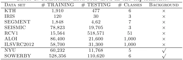
In this subsection, we first demonstrate our motivation on the recognition of human action (Sch¨uldt et al., 2004). We then consider a variety of benchmark multiclass data sets with-out background from the LIBSVM website4 to evaluate the performance of the proposed algorithms for multiclass classification. Lastly, we conduct experiments on two multiclass data sets with background collected from Silberman et al. (2012) and He et al. (2004). The training/testing partition is either predefined or the data is randomly split into 80% train-ing and 20% testtrain-ing. The statistics of each data set are reported in Table 1. We compare our algorithms with some baseline methods: OVO, OVR, ECOC (Dietterich and Bakiri, 1995) and Top-kSVM (Lapin et al., 2015, 2016). The library for ECOC is from Pedregosa et al. (2011) and the size of code for ECOC is selected using 5-fold cross validation over the range{2,10,30,50}. Top-kSVM (Lapin et al., 2015, 2016) is one of the state-of-the-art generalized multiclass SVM for top-k error optimization. The code is provided by their authors. Following the similar parameter settings in Lapin et al. (2015, 2016) for Top-k
SVM,k is selected using 5-fold cross validation over the range{1,3,5,10}.
Table 1: Multiclass data sets used in the experiments. Data set # TRAINING # TESTING # Classes Background
KTH 1,910 477 6 ×
IRIS 120 30 3 ×
SEGMENT 1,848 4,62 7 ×
SEISMIC 78,823 19,705 3 ×
RCV1 15,564 518,571 51 ×
ALOI 86,400 21,600 1,000 ×
ILSVRC2012 58,700 31,300 1,000 ×
NYU 60,232 11,768 5 √
SOWERBY 528,356 110,620 6
√
Table 2: Testing error rate (in %) on the KTH data set.
OVO OVR ECOC Top-kSVM CCMC CCMC-Greedy CCMC-DP
8.81 8.18 7.73 8.13 7.34 6.29 5.66
7.1.1 Human action recognition
We first validate our methods by recognizing complex human actions on the KTH data set Sch¨uldt et al. (2004). KTH contains six types of human action: walk,jog,run,hand wave,
hand clapandboxing. The confusion matrix of OVR on the KTH data set is shown in Figure 1. From Figure 1, we can see that it is easy to identifywalk from other actions, whereas it is difficult to distinguish betweenboxing andhand clap. This observation is consistent with commonsense. Our model aims to classify classes from simple to hard; the classifier of the hard actions will benefit significantly from the prediction of the simple actions.
The testing error rates of the different methods are shown in Table 2. The order of actions identified by CCMC-Greedy is: run, hand wave, walk, jog, boxing and hand clap. CCMC-DP finds the action order: walk,run,jog, hand wave,boxing and hand clap. From these results, we observe that:
• For the KTH data set, our methods achieve a better prediction performance than OVO, OVR, ECOC and Top-k SVM, which verifies that our model effectively uses the predictions of previous classifiers to improve the performance of OVR.
• CCMC-Greedy and CCMC-DP improve CCMC, which also verifies our motivation: we should classify the classes from easy to hard. The order of actions (from easy to hard) found by CCMC-Greedy and CCMC-DP are consistent with the confusion matrix, which demonstrates that our model can automatically identify easy and hard classes, and use the predictions of classifiers from easier classes to train the classifier for harder classes.
Figure 3: Confusion Matrix of CCMC-DP on the KTH Data Set.
7.1.2 Results without background data
We compare OVO, OVR and ECOC with our algorithms on the benchmark data sets without background. The classification results for our methods and baseline approaches on the IRIS, SEGMENT, SEISMIC and RCV1 data sets are reported in Table 3. Based on these results, we make the following observations.
• Our results show that OVR and OVO perform as accurate as ECOC and Top-k
SVM, which is consistent with the empirical results in Rifkin and Klautau (2004), Demirkesen and Cherifi (2008) and Lapin et al. (2015, 2016).
• CCMC consistently improves the prediction performance of OVR and other baselines on all data sets. The results verify Rifkin and Klautau (2004)’s conjecture: an algo-rithm which exploits the relationship between classes can offer superior performance.
• When OVO outperforms OVR on certain data sets such as SEISMIC and SEGMENT, our methods are able to achieve superior prediction performance to OVO on these data sets.
• CCMC-Greedy is better than CCMC, and CCMC-DP outperforms CCMC-Greedy and CCMC. The results validate our theoretical analysis: i) Class order affects the performance of CCMC. ii) CCMC-DP is able to find the globally optimal CCMC which achieves the best prediction performance compared to CCMC-Greedy and CCMC. iii) The CCMC-Greedy algorithm achieves comparable prediction performance with CCMC-DP.
We also evaluate the performance of our fast greedy algorithm on the ALOI data set, which contains 1,000 classes. Here, ω is set to 10, 30, 50 and 100. The classification results and training time are reported in Table 4, from which we can see that CCMC-FG outperforms CCMC and improves the prediction performance of OVR, ECOC and Top-k
Table 3: Testing error rate (in %) on data sets without background.
CCMC-Data set OVO OVR ECOC Top-kSVM CCMC Greedy DP
IRIS 10.00 10.00 8.67 10.33 3.33 3.33 3.33
SEGMENT 5.63 7.14 7.08 7.06 6.28 5.63 5.19
SEISMIC 27.92 29.87 27.62 28.19 26.85 26.50 26.48
RCV1 11.09 11.90 11.83 11.98 11.78 11.71 11.68
Table 4: Testing error rate (in %) and training time (in second) on the ALOI data set.
Method Testing Error Training Time
OVO 6.88 14,748s
OVR 13.69 1,559s
ECOC 10.31 85,316s
Top-kSVM 9.4 65s
CCMC 5.46 12,715s
CCMC-FG(ω= 10) 5.27 16,327s
CCMC-FG(ω= 30) 5.08 31,886s
CCMC-FG(ω= 50) 4.94 67,582s
CCMC-FG(ω= 100) 4.78 163,891s
7.1.3 Results with background data
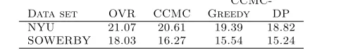
The OVO, ECOC and Top-k SVM approaches cannot be directly applied to background data. Table 5 shows the classification results for our methods and OVR on the NYU and SOWERBY data sets. From the results of Table 5, we can see that:
• CCMC consistently outperforms OVR.
• CCMC-Greedy achieves better prediction performance than CCMC and is comparable to CCMC-DP.
• CCMC-DP improves the prediction performance of OVR on the data sets with back-ground by 3%.
7.1.4 Training time
This section studies the training time of the proposed methods and baselines on all data sets. The results are shown in Tables 4 and 6. From these results, we can see that:
• Top-kSVM is much faster than other methods on the ALOI data set with 1000 classes.
• Compared to OVR, CCMC maintains the training time over an acceptable threshold, while CCMC consistently improves OVR.
Table 5: Testing error rate (in %) on data sets with background.
CCMC-Data set OVR CCMC Greedy DP
NYU 21.07 20.61 19.39 18.82
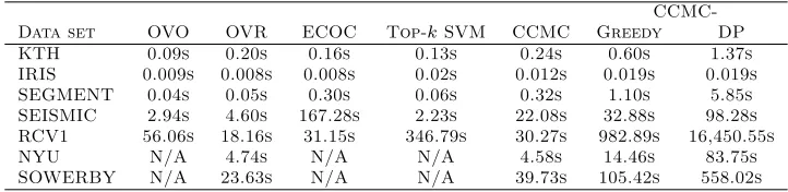
Table 6: Training time (in second).
CCMC-Data set OVO OVR ECOC Top-kSVM CCMC Greedy DP
KTH 0.09s 0.20s 0.16s 0.13s 0.24s 0.60s 1.37s
IRIS 0.009s 0.008s 0.008s 0.02s 0.012s 0.019s 0.019s
SEGMENT 0.04s 0.05s 0.30s 0.06s 0.32s 1.10s 5.85s
SEISMIC 2.94s 4.60s 167.28s 2.23s 22.08s 32.88s 98.28s
RCV1 56.06s 18.16s 31.15s 346.79s 30.27s 982.89s 16,450.55s
NYU N/A 4.74s N/A N/A 4.58s 14.46s 83.75s
SOWERBY N/A 23.63s N/A N/A 39.73s 105.42s 558.02s
• CCMC-Greedy is much faster than CCMC-DP.
• With the increasing value ofω, the training time of CCMC-FG rises, but the prediction performance of CCMC-FG becomes better. ω can be set according to the time and accuracy requirements of applications.
The testing time of the proposed methods is similar to OVR. Although the training time of the proposed approaches is slower than OVR, the time required to test is of more importance than the time required to train for many applications.
7.1.5 Comparisons with deep learning methods
ADIOS (Ciss´e et al., 2016) is a state-of-the-art deep learning architecture for solving multiple class and label tasks. Unlike traditional deep learning methods that use a flat output layer, ADIOS aims to capture the complex dependency between labels/classes to improve deep learning methods. Their approach is to split the label/class set into two subsets, G1 and G2, such that given G1, the labels/classes inG2 are independent. Our strategy to leverage label/class dependency is very different from that of ADIOS, as shown in Figure 2, we use a classifier chain model for multi-class classification and find the optimal class ordering. After that, we use the predictions of classifiers from easier classes to train the classifiers for harder classes. As such, the assumptions and constraints used in ADOIS are not applicable in our model.
This subsection conducts the experiments on the ILSVRC2012 data set5. It con-tains 1,000 object categories (Liu et al., 2017). Due to the limit of computational re-sources, we randomly sample 58,700 training instances and 31,300 testing instances from the ILSVRC2012 data set. We use the source code provided by the authors of ADIOS with default parameters. According to Ciss´e et al. (2016), we use one hidden layer with 1024 rectified linear units (ReLUs) (Glorot et al., 2011) between inputs and G1, and another 512-dimensional ReLUs between the hidden layer before G1 and G2 as well as direct con-nections betweenG1 andG2. We also compare with VGG (Simonyan and Zisserman, 2014) and residual nets (ResNet) (He et al., 2016). Both VGG and ResNet use a flat output layer, in which do not model the dependency between the classes(Ciss´e et al., 2016), so the rich structure information among classes is missing in VGG and ResNet. We use the source code provided by the respective authors with default parameters. Following He et al. (2016), we use the 34-layer residual nets due to the limit of computational resources, and also extract
Table 7: Testing error rate (in %) of VGG, ResNet-34, ADIOS and CCMC-FG on the ILSVRC2012 data set.
Method VGG ResNet-34 ADIOS CCMC-FG+VGG features CCMC-FG+ResNet features
Testing Error 23.95 21.51 21.28
23.98 (ω= 10) 21.85 (ω= 10) 22.67 (ω= 30) 20.11 (ω= 30) 20.73 (ω= 50) 19.84 (ω= 50)
2048-dimensional features by the ResNet-34. According to Simonyan and Zisserman (2014), we extract 4096-dimensional features from the 16-layer of the VGG. Here,ωis set to 10, 30 and 50 for our method.
The classification results are reported in Table 7. From this table, we can observe that
• ADIOS outperforms VGG and ResNet-34, which verifies ADIOS’s claim: existing deep learning approaches do not take into account the often unknown but nevertheless rich relationships between classes, this knowledge about the rich class structure (and other deep structure in data) is sometime referred to as dark knowledge (e.g. by Hinton et al. (2015) and Ba and Caruana (2014)).
• Without the restriction of the assumptions and constraints used in ADOIS, our method achieves better performance than ADIOS with the increasing value ofω.
• CCMC-FG with ResNet features obtains better performance than CCMC-FG with VGG features, which demonstrates that our proposed method can be further improved based on better features.
• Based on the deep learning features, CCMC-FG consistently improves VGG and ResNet-34 with the increasing value of ω. The results validate our analysis and the better ordering of classes obtains the better performance. Note that the above men-tioned results were obtained using 58,700 training data points. We conclude that with limited data, the usage of structure information is helpful. We conjecture that this advantage may ultimately vanish as more and more data becomes available for training.
7.2 Experiment on Multi-label Classification
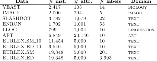
We conduct experiments on ten real-world multi-label data sets with various domains from three websites.678 The EURLEX SM and EURLEX ED data sets are preprocessed accord-ing to the experimental settaccord-ings in Dembczynski et al. (2010) and Zhang and Schneider (2012). The statistics of data sets are presented in Table 8. We compare our algorithms with some baseline methods: BR, CC, ECC, CCA (Zhang and Schneider, 2011) and MMOC (Zhang and Schneider, 2012). ECC is averaged over several CC predictions with random
6. http://mulan.sourceforge.net
7. http://meka.sourceforge.net/#datasets
Table 8: Multi-label data sets used in the experiments.
Data # inst. # attr. # labels Domain
YEAST 2,417 103 14 biology
IMAGE 2,000 294 5 image
SLASHDOT 3,782 1,079 22 text
ENRON 1,702 1,001 53 text
LLOG 799 1,004 10 linguistics
ART 6,849 23,146 10 art
EURLEX SM 10 11,454 5,000 10 text
EURLEX ED 10 6,540 5,000 10 text
EURLEX SM 19,348 5,000 201 text
EURLEX ED 19,348 5,000 3,993 text
order and the ensemble size in ECC is set to 10 according to Dembczynski et al. (2010); Read et al. (2009). In our experiment, the running time of PCC and EPCC (Dembczynski et al., 2010) on most data sets, like SLASHDOT and ART, takes more than one week. From the results in Dembczynski et al. (2010), ECC is comparable with EPCC and outperforms PCC, so we do not consider PCC and EPCC here. CCA and MMOC are two state-of-the-art encoding-decoding (Hsu et al., 2009) methods. We cannot get the results of CCA and MMOC on ART , EURLEX SM 10 and EURLEX ED 10 data sets in one week.
We consider the following evaluation measurements Mao et al. (2013) to measure the prediction performance of all methods fairly:
• Example-F1: computes the F-1 score for all the labels of each testing example and then takes the average of the F-1 score.
• Macro-F1: calculates the F-1 score for each label and then takes the average of the F-1 score.
• Micro-F1: computes true positives, true negatives, false positives and false negatives over all labels, and then calculates an overall F-1 score.
The larger the value of those measurements, the better the performance. We perform 5-fold cross-validation on each data set and report the mean and standard error of each evaluation measurement.
7.2.1 Small-scale results
Three measurement results for CC-Greedy, CC-DP and baseline approaches in respect to the different small-scale data sets are reported in Tables 9, 10 and 11. We conduct the pairwise t-test at a 5% significance level to show that our methods perform significantly better than the compared methods. From the results, we can see that:
Table 9: Results of Example-F1 on the various small-scale data sets (mean ± standard deviation). The best results are in bold. Numbers in square brackets indicate the rank. “-” denotes the training time is more than one week.
Data set BR CC ECC CCA MMOC CC-Greedy CC-DP
YEAST 0.6076±0.02[6] 0.5850±0.03[7] 0.6096±0.02[5] 0.6109±0.02[4] 0.6132±0.02[3] 0.6144±0.02[1] 0.6135±0.02[2] IMAGE 0.5247±0.03[7] 0.5991±0.02[1] 0.5947±0.02[4] 0.5947±0.01[4] 0.5960±0.01[3] 0.5939±0.02[6] 0.5976±0.02[2] SLASHDOT 0.4898±0.02[6] 0.5246±0.03[4] 0.5123±0.03[5] 0.5260±0.02[3] 0.4895±0.02[7] 0.5266±0.02[2] 0.5268±0.02[1] ENRON 0.4792±0.02[7] 0.4799±0.01[6] 0.4848±0.01[4] 0.4812±0.02[5] 0.4940±0.02[1] 0.4894±0.02[2] 0.4880±0.02[3] LLOG 0.3138±0.02[6] 0.3219±0.03[4] 0.3223±0.03[3] 0.2978±0.03[7] 0.3153±0.03[5] 0.3269±0.02[2] 0.3298±0.03[1] ART 0.4840±0.02[5] 0.5013±0.02[4] 0.5070±0.02[3] - - 0.5131±0.02[2] 0.5135±0.02[1] EURLEX SM 10 0.8594±0.00[5] 0.8609±0.00[1] 0.8606±0.00[3] - - 0.8600±0.00[4] 0.8609±0.00[1] EURLEX ED 10 0.7170±0.01[5] 0.7176±0.01[4] 0.7183±0.01[2] - - 0.7183±0.01[2] 0.7190±0.01[1]
Average Rank 5.88 3.88 3.63 4.60 3.80 2.63 1.50
Table 10: Results of Macro-F1 on the various small-scale data sets (mean ±standard de-viation). The best results are in bold. Numbers in square brackets indicate the rank. “-” denotes the training time is more than one week.
Data set BR CC ECC CCA MMOC CC-Greedy CC-DP
YEAST 0.3543±0.01[4] 0.3993±0.03[1] 0.3763±0.02[2] 0.3496±0.02[5] 0.3431±0.02[7] 0.3441±0.02[6] 0.3596±0.02[3] IMAGE 0.5852±0.01[7] 0.6013±0.02[1] 0.5988±0.01[4] 0.6010±0.01[2] 0.5975±0.01[6] 0.5987±0.02[5] 0.6010±0.01[2] SLASHDOT 0.3416±0.01[4] 0.3485±0.02[2] 0.3331±0.01[7] 0.3512±0.02[1] 0.3334±0.01[6] 0.3431±0.01[3] 0.3408±0.01[5] ENRON 0.2089±0.02[2] 0.2066±0.02[5] 0.2088±0.02[3] 0.1594±0.03[6] 0.1539±0.02[7]0.2090±0.02[1] 0.2082±0.02[4] LLOG 0.3452±0.03[2] 0.3428±0.03[4] 0.3425±0.04[5] 0.3189±0.04[7] 0.3303±0.04[6] 0.3448±0.03[3] 0.3471±0.04[1] ART 0.4836±0.01[4] 0.4816±0.01[5] 0.4851±0.02[3] - - 0.4876±0.01[2] 0.4884±0.02[1] EURLEX SM 10 0.8546±0.00[5] 0.8558±0.00[2] 0.8554±0.00[3] - - 0.8550±0.00[4] 0.8559±0.00[1] EURLEX ED 10 0.7201±0.01[5] 0.7202±0.01[4] 0.7205±0.01[3] - - 0.7208±0.01[2] 0.7217±0.01[1]
Average Rank 4.13 3.00 3.75 4.20 6.40 3.25 2.25
• CC improves on the performance of BR, however, it underperforms compared to ECC. This result verifies the answer to our first question stated in Section 2.2: the label order does affect the performance of CC; ECC, which averages over several CC predictions with random order, improves the performance of CC.
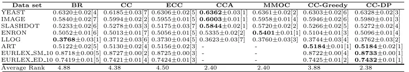
Table 11: Results of Micro-F1 on the various small-scale data sets (mean ± standard de-viation). The best results are in bold. Numbers in square brackets indicate the rank. “-” denotes the training time is more than one week.
Data set BR CC ECC CCA MMOC CC-Greedy CC-DP
YEAST 0.6320±0.02[4] 0.6185±0.03[7] 0.6306±0.02[5]0.6362±0.03[1] 0.6361±0.02[2] 0.6303±0.02[6] 0.6328±0.02[3] IMAGE 0.5840±0.02[7] 0.5994±0.02[2] 0.5955±0.01[5]0.6003±0.01[1] 0.5958±0.01[4] 0.5946±0.02[6] 0.5980±0.01[3] SLASHDOT 0.5233±0.02[6] 0.5278±0.03[3] 0.5175±0.03[7]0.5844±0.02[1] 0.5720±0.02[2] 0.5266±0.02[5] 0.5272±0.02[4] ENRON 0.5052±0.01[6] 0.5013±0.01[7] 0.5056±0.01[5] 0.5335±0.02[2] 0.5401±0.01[1] 0.5104±0.01[3] 0.5096±0.01[4] LLOG 0.3768±0.03[1] 0.3712±0.03[6] 0.3730±0.04[5] 0.3623±0.03[7] 0.3760±0.03[3] 0.3744±0.03[4] 0.3762±0.03[2] ART 0.5122±0.02[5] 0.5130±0.02[4] 0.5156±0.02[3] - - 0.5184±0.01[1]0.5184±0.02[1] EURLEX SM 10 0.8718±0.00[5] 0.8727±0.00[2] 0.8725±0.00[3] - - 0.8722±0.00[4] 0.8733±0.00[1] EURLEX ED 10 0.7419±0.01[5] 0.7421±0.01[4] 0.7424±0.01[3] - - 0.7425±0.01[2] 0.7432±0.01[1]
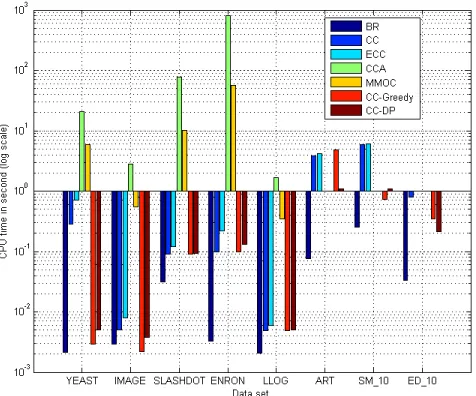
Figure 4: Training time (in second) of all methods on the small-scale data sets. EU-RLEX SM 10 and EUEU-RLEX ED 10 are abbreviated to SM 10 and ED 10.
Figure 5: Testing time (in second) of all methods on the small-scale data sets. EU-RLEX SM 10 and EUEU-RLEX ED 10 are abbreviated to SM 10 and ED 10.
• Our proposed CC-DP and CC-Greedy algorithms are successful on most data sets. This empirical result verifies the effectiveness of our easy-to-hard learning strategies, and we provide an answer to the last two questions stated in Section 2.2: a globally optimal CC exists and CC-DP is able to find the globally optimal CC that achieves the best prediction performance. The CC-Greedy algorithm achieves comparable prediction performance with CC-DP.
Figures 4 and 5 show the training and testing time of CC-Greedy, CC-DP and the baseline methods on the small-scale data sets, respectively. According to these two figures, we can see that:
• Our proposed algorithms are much faster than CCA and MMOC in terms of both training and testing time.
• CC-Greedy and CC-DP achieve comparable testing time with BR, CC and ECC. Though the training time of our algorithms are slower than BR, CC and ECC, our extensive empirical studies show that our algorithms achieve superior prediction per-formance than those baselines.
• The CC-Greedy algorithm is much faster than CC-DP in terms of training time, and it achieves comparable prediction performance with CC-DP.
7.2.2 Large-scale results
This subsection studies the performance of Tree-Greedy, Tree-DP and other baselines on the EURLEX SM and EURLEX ED data sets with many labels. We cannot get the results of CCA and MMOC on EURLEX SM and EURLEX ED data sets in one week. And we also cannot get the results of ECC on EURLEX ED data set in one week. The prediction performance of Tree-Greedy, Tree-DP and the baselines are reported in Tables 12, 13 and 14. We conduct the pairwise t-test at a 5% significance level to show that our methods perform significantly better than the compared methods. From the results, we can see that: our proposed Tree-Greedy and Tree-DP algorithms consistently outperform BR, CC and ECC on the data sets with many labels.
The training and testing time of Tree-Greedy, Tree-DP and the baselines on the EU-RLEX SM and EUEU-RLEX ED data sets are shown in Figure 6. According to this figure, we can observe that compared to BR, CC and ECC, our algorithms maintain the testing time over an acceptable threshold, while our methods are much faster than the baselines in terms of training time.
7.3 Experiment on Ordinal Classification
This subsection conducts experiments on four ordinal data sets with various domains from website9. The statistics of these data sets are presented in Table 15. We compare our algorithm with some baseline methods: SVM (Shashua and Levin, 2002), MAP (Chu and Ghahramani, 2005), EP (Chu and Ghahramani, 2005) and BD (Destercke and Yang, 2014).
Table 12: Results of Example-F1 on EURLEX SM and EURLEX ED data sets (mean ± standard deviation). The best results are in bold. Numbers in square brackets indicate the rank. “-” denotes the training time is more than one week.
Data set BR CC ECC Tree-Greedy Tree-DP
EURLEX SM 0.6970±0.02[5] 0.7233±0.01[4] 0.7263±0.01[3]0.7292±0.01[2] 0.7301±0.01[1] EURLEX ED 0.4345±0.03[4] 0.4528±0.02[3] - 0.4550±0.01[2] 0.4563±0.01[1]
Average Rank 4.5 3.5 3 2 1
Table 13: Results of Macro-F1 on EURLEX SM and EURLEX ED data sets (mean± stan-dard deviation). The best results are in bold. Numbers in square brackets indi-cate the rank. “-” denotes the training time is more than one week.
Data set BR CC ECC Tree-Greedy Tree-DP
EURLEX SM 0.4777±0.02[5] 0.4785±0.02[4] 0.4800±0.02[3]0.4817±0.01[2] 0.4834±0.01[1] EURLEX ED 0.1660±0.01[4] 0.1812±0.00[3] - 0.1844±0.00[2] 0.1848±0.00[1]
Average Rank 4.5 3.5 3 2 1
The results are shown in Table 16. From this table, we can see that our proposed CCMC-DP outperforms the other baselines on all data sets, which verifies that our method is able to capture and use the correlated information between ordinal classes, and boost the performance of ordinal classification problems.
7.4 Experiment on Relationship Prediction
This subsection conducts experiments on the Epinions data set (Massa and Avesani, 2006). According to Chiang et al. (2015), we collect 10,000 users and 41 features in this data set. We compare our proposed Tree-DP algorithm with some popular methods: IMC (Jain and Dhillon, 2013), MF-ALS (Hsieh et al., 2012), HOC-3 (Chiang et al., 2014), HOC-5 (Chiang et al., 2014) and DirtyIMC (Chiang et al., 2015). We perform 5-fold cross-validation on this data set and report the mean and standard error of Example-F1. The results are shown in Table 17. From this table, we can see that 1) DirtyIMC outperforms the other baselines, which verifies the effectiveness of using feature information and is consistent with the empirical results in Chiang et al. (2015). 2) Our proposed Tree-DP algorithm is able to achieve the best accuracy among all baselines, which demonstrates the superior performance of the easy-to-hard learning strategy.
8. Conclusion
Table 14: Results of Micro-F1 on EURLEX SM and EURLEX ED data sets (mean± stan-dard deviation). The best results are in bold. Numbers in square brackets indi-cate the rank. “-” denotes the training time is more than one week.
Data set BR CC ECC Tree-Greedy Tree-DP
EURLEX SM 0.7321±0.01[5] 0.7422±0.02[3] 0.7363±0.01[4]0.7440±0.01[2] 0.7454±0.01[1] EURLEX ED 0.4200±0.01[4] 0.4477±0.01[3] - 0.4527±0.00[2] 0.4549±0.00[1]
Average Rank 4.5 3 4 2 1
Figure 6: Training and testing time (in second) of BR, CC, ECC, Tree-Greedy and Tree-DP on EURLEX SM and EURLEX ED data sets.
multiclass classification (CCMC) to transfer class information between classifiers. Then, we generalize the CCMC model over a random class order and provide a theoretical analysis of the generalization error for the proposed generalized model. Our results show that the upper bound of the generalization error depends on the sum of the reciprocal of the square of the margin over the classes. Based on our results, we propose the easy-to-hard learning paradigm for multiclass classification to automatically identify easy and hard classes and then use the predictions from simpler classes to help solve harder classes.