A Random Matrix Analysis and Improvement of Semi-Supervised Learning for Large Dimensional Data

A Random Matrix Analysis and Improvement of

Semi-Supervised Learning for Large Dimensional Data

Xiaoyi Mai [email protected]

Romain Couillet [email protected]

CentraleSup´elec

Universit´e Paris-Saclay

Laboratoire des Signaux et Syst`emes 3 rue Joliot Curie, 91192 Gif-Sur-Yvette

Editor:Nicolas Vayatis

Abstract

This article provides an original understanding of the behavior of a class of graph-oriented semi-supervised learning algorithms in the limit of large and numerous data. It is demon-strated that the intuition at the root of these methods collapses in this limit and that, as a result, most of them become inconsistent. Corrective measures and a new data-driven parametrization scheme are proposed along with a theoretical analysis of the asymptotic performances of the resulting approach. A surprisingly close behavior between theoretical performances on Gaussian mixture models and on real data sets is also illustrated through-out the article, thereby suggesting the importance of the proposed analysis for dealing with practical data. As a result, significant performance gains are observed on practical data classification using the proposed parametrization.

Keywords: semi-supervised learning, kernel methods, random matrix theory, high di-mensional statistics

1. Introduction

Semi-supervised learning consists in classification schemes combining few labelled and nu-merous unlabelled data. With the advent of the big-data paradigm, where supervised learning implies the impossible pre-labelling of sometimes millions of samples, these so-far marginal methods are attracting a renewed attention. Its appeal also draws on its provid-ing an alternative to unsupervised learnprovid-ing which excludes the possibility to exploit known data. We refer to Chapelle et al. (2006) for an overview.

An important subset of semi-supervised learning methods concerns graph-based ap-proaches. In these, one considers data instances x1,· · · , xn ∈ Rp as vertices on a graph with edge weights Wij encoding their similarity, which is usually defined through a kernel

function f, as with radial kernels of the type Wij =f(kxi−xjk2/p) which we shall focus

on in this article. The motivation follows from one’s expectation that two instances with a strong edge weight tend to belong to the same class and thus vertices of a common class tend to aggregate. Standard methods for recovering the classes of the unlabelled data then consist in various random walk (Jaakkola and Szummer, 2002) or label propagation (Zhu and Ghahramani, 2002) algorithms on the graph which softly allocate “scores” for each

c

node to belong to a particular class. These scores are then compared for each class in order to obtain a hard decision on the individual unlabelled node class. A popular, and widely recognized as highly performing, example is the PageRank approach (Avrachenkov et al., 2011).

Many of these algorithms also have the particularity of having a closed-form and quite interrelated expression for their stationary points. These stationary points are also often found to coincide with the solutions to optimization problems under constraints, indepen-dently established. This is notably the case of Zhu et al. (2003) under equality constraints for the labelled nodes or of Belkin et al. (2004) where a relaxation approach is used instead to allow for modifications of the value of labelled nodes – this ensuring that erroneously labelled data or poorly informative labelled data do not hinder the algorithm performance. As is often the case in graph-related optimization, a proper choice of the matrix represen-tative of the inter-data affinity is at the core of scientific research and debates and mainly defines the differences between any two schemes. In particular, Joachims et al. (2003) sug-gests the use of a standard Laplacian representative, where Zhou et al. (2004) advises for a normalized Laplacian approach. These individual choices correspondingly lead to different versions of the label propagation methods on the graph, as discussed in Avrachenkov et al. (2011).

There also exists another branch of manifold based semi-supervised learning (Belkin and Niyogi, 2004; Goldberg et al., 2009; Moscovich et al., 2016). In contrast to the methods discussed in this paper, these approaches involve a step of manifold learning, which plays a decisive role in the success of the learning task. While there exist many articles pro-viding theoretical analyses for such methods (Wasserman and Lafferty, 2008; Bickel et al., 2007; Moscovich et al., 2016; Globerson et al., 2017), a comprehensive comparison to the graph-based methods presently discussed is beyond current analytical reach. This being said, while the Gaussian-mixture data model under study in the present article violates the manifold assumption, given appropriate feature (kernel function) mapping, there ex-ists a low dimensional manifold where data demonstrate a clustering behavior, as shown by Couillet and Benaych-Georges (2015); as such, when the classes are very well sepa-rated and sufficient data are available to estimate the manifold, manifold-based methods in this setting should lead to competitive performance. While clearly out of our present scope, future investigations might allow for a comparative study of manifold versus graph approaches. Another recent line of alternative works consider SSL from a graph signal pro-cessing perspective (Narang et al., 2013a,b; Gadde et al., 2014; Anis et al., 2015), where the classification scores are viewed as smooth signals on the similarity graph and the learning task then consists in recovering a bandlimited (understood in the graph Fourier transform domain) graph signal from its known sample values.

and proposes instead to derive, for the first time to the best of the authors’ knowledge, theoretical results on the performance of the aforementioned algorithms in the large n, p

limit for a certain class of statistically distributed data x1, . . . , xn ∈ Rp. Precisely due to the large data assumption, as we shall observe, most of the intuition leading up to the aforementioned algorithms collapse as n, p→ ∞ at a similar rate, and we shall prove that few algorithms remain consistent in this regime.

Specifically, recall that the idea behind graph-based semi-supervised learning is to exploit the similarity between data points and thus expect a clustering behavior of close-by data nodes. In the large data assumption (i.e., p 1), this similarity-based approach suffers a curse of dimensionality. As the span of Rp grows exponentially with the data dimension

p, when p is large, the data points xi (if not too structured) are in general so sparsely

distributed that their pairwise distances tend to be similar regardless of their belonging to the same class or not. The Gaussian mixture model that we define in Subsection 3 and will work on is a telling example of this phenomenon; as we show, in a regime where the classes ought to be separable (even by unsupervised methods as shown by Couillet and Benaych-Georges 2015), the normalized distancekxi−xjk/

√

pof two random different data instances

xi and xj generated from this model converges to a constantirrespective of the class of xi

and xj in the Gaussian mixture and, consequently, the similarity defined byWij =f(kxi−

xjk2/p) is asymptotically the same for all pairs of data instances. This behavior should

therefore invalidate the intuition behind semi-supervised classification, hence likely render graph-based methods ineffective. As a direct consequence, the scores are flat in the sense that they have the same asymptotic values, irrespective of the class. Nonetheless, we will show that sensible classification on data sets generated from this model can still be achieved provided that appropriate amendments to the classification algorithms are enforced, due to the small fluctuations around these flat asymptotic limit of scores. This flat limit is reminiscent of the work by Nadler et al. (2009) where the authors show that the scores indeed share the same limit, irrespective of the class, in the presence of infinitely many unlabelled samples but for p ≥ 2 fixed. Yet, despite the scores flatness, the authors experimentally observed non-trivial classification in binary tasks thanks to the small difference between scores; they however did not provide any theoretical support for such behavior, for they analysis failed to recover the small fluctuations.

Inspired by Avrachenkov et al. (2011), we generalize here the algorithm proposed in Zhu et al. (2003) by introducing a normalization parameter α in the cost function in order to design a large class of regularized affinity-based methods, among which are found the tradi-tional Laplacian- and normalized Laplacian-based algorithms. The generalized optimization framework is presented in Section 2.

The main contribution of the present work is to provide a quantitative performance study of the generalized graph-based semi-supervised algorithm for large dimensional Gaussian-mixture data and radial kernels, technically following the random matrix approach de-veloped by Couillet and Benaych-Georges (2015). Our main findings are summarized as follows:

to be classified into the class with most labelled nodes; we propose a normalization update of the standard algorithms to correct this limitation.

• Once the aforementioned bias corrected, the choice of the affinity matrix (and thus of the parameter α) strongly impacts the performances; most importantly, within our framework, both standard Laplacian (α = 0 here) and normalized Laplacian-based (α = −1₂) methods, although widely discussed in the literature, fail in the large dimensional data regime. Of the family of algorithms discussed above, only the PageRank approach (α=−1) is shown to provide asymptotically acceptable results.

• The scores of belonging to each class attributed to individual nodes by the algorithms are shown to asymptotically follow aGaussian distribution with mean and covariance depending on the statistical properties of classes, the ratio of labelled versus unlabelled data, and the value of the first derivatives of the kernel function at the limiting value

τ of 1_pkxi −xjk2 (which we recall is irrespective of the genuine classes of xi, xj).

This last finding notably allows one to predict the asymptotic performances of the semi-supervised learning algorithms.

• From the latter result, three main outcomes unfold:

– when three classes or more are considered, there exist Gaussian mixture models for which classification is shown to be impossible;

– despite PageRank’s consistency, we further justify that the choice α = −1 is not in general optimal. For the case of 2-class learning, we provide a method to approach the optimal value ofα; this method is demonstrated on real data sets to convey sometimes dramatic improvements in correct classification rates.

– for a 2-class learning task, necessary and sufficient conditions for asymptotic consistency are: f0(τ) < 0, f00(τ) > 0 and f00(τ)f(τ) > f0(τ)2; in particular, Gaussian kernels, failing to meet the last condition, cannot deal with the large dimensional version of the “concentric spheres” task.

Throughout the article, theoretical results and related discussions are confirmed and illustrated with simulations on Gaussian-mixture data as well as the popular MNIST data (LeCun et al., 1998), which serves as a comparison for our theoretical study on real world data sets. The consistent match of our theoretical findings on MNIST data, despite their departing from the very large dimensional and Gaussian-mixture assumption, suggests that our results have a certain robustness to these assumptions and can be applied to a larger range of data. We indeed believe that, while only the limiting behavior of Gaussian mixture inputs is characterized in this article (mostly for technical reasons), the analysis reveals certain properties inherent to graph-based SSL methods, which extend well beyond the Gaussian hypothesis.

Notations: δb_a is a binary function taking the value of 1 if a=b or that of 0 if not. 1n

is the column vector of ones of size n,In then×nidentity matrix. The norm k · kis the

Euclidean norm for vectors and the operator norm for matrices. The operator diag(v) = diag{va}ka=1 is the diagonal matrix havingv1, . . . , vk as its ordered diagonal elements. O(·)

variable x ≡ xn and un ≥ 0, we write x = O(un) if for any η > 0 and D > 0, we have

nDP(x ≥ nηun) → 0. When multidimensional objects are concerned, for a vector (or a

diagonal matrix)v, v = O(un) means the maximum entry in absolute value is O(un) and

for a square matrixM,M =O(un) means that the operator norm ofM isO(un).

2. Optimization Framework

Letx1, . . . , xn∈Rp be ndata vectors belonging to K classesC1, . . . ,CK. The class

associ-ation of the n[l] vectorsx1, . . . , xn[l] is known (these vectors will be referred to aslabelled),

while the class of the remaining n[u] vectors xn[l]+1, . . . , xn (n[l] +n[u] = n) is unknown

(these are referred to asunlabelled vectors). Within both labelled and unlabelled subsets, the data are organized in such a way that then[l]1 first vectorsx1, . . . , xn[l]1 belong to class C1,n[l]2subsequent vectors toC2, and so on, and similarly for then[u]1, n[u]2, . . .first vectors of the setxn[l]+1, . . . , xn. Note already that this ordering is for notational convenience and

shall not impact the generality of our results.

The affinity relation between the vectors x1, . . . , xnis measured from the weight matrix

W defined by

W ≡

f

1

pkxi−xjk

2

n

i,j=1

for some function f. The matrix W may be seen as the adjacency matrix of the n-node graph indexed by the vectorsx1, . . . , xn. We further denote byDthe diagonal matrix with

Dii≡di =Pnj=1Wij the degree of the node associated toxi.

We next define a score matrix F ∈_Rn×K with Fik representing the evaluated score for

xi to belong to Ck. In particular, following the conventions typically used in graph-based

semi-supervised learning (Chapelle et al., 2006), we shall affect a unit scoreFik = 1 ifxi is

a labelled data of class C_k and a null score for all Fik0 with k0 6=k. In order to attribute

classes to the unlabelled data, scores are first affected by means of the resolution of an optimization framework. We propose here

F = argmin_F∈Rn×k K

X

k=1

n

X

i,j=1

Wij

dα_iF_ik−dα_jF_jk

2

s.t. Fik=

(

1, ifxi ∈ Ck

0, otherwise,1≤i≤n[l],1≤k≤K (1) where α ∈ _R is a given parameter. The interest of this generic formulation is that it coincides with the standard Laplacian-based approach for α = 0 and with the normalized Laplacian-based approach forα=−1₂, both discussed in Section 1. Note importantly that Equation (1) is naturally motivated by the observation that large values ofWij enforce close

values for Fik and Fjk while small values for Wij allow for more freedom in the choice of

Fik and Fjk.

By denoting

F =

F[l]

F[u]

, W =

W[ll] W[lu]

W[ul] W[uu]

, and D=

D[l] 0 0 D[u]

with F_[l] ∈ _Rn[l]_{, W}

[ll] ∈ Rn[l]×n[l], D[l] ∈ Rn[l]×n[l], one easily finds (since the problem is a convex quadratic optimization with linear equality constraints) the solution to (1) is explicitly given by

F_[u]=Inu−D

−1−α

[u] W[uu]D[αu]

−1

D_[−_u1_]−αW_[ul]Dα_[l]F_[l]. (2) Once these scores are affected, a mere comparison between all scoresFi1, . . . , FiK for

unla-belled data xi (i.e., for i > n[l]) is performed to decide on its class, i.e., the allocated class index ˆCxi for vectorxi is given by

ˆ

Cxi =Cˆ_k for ˆk= argmax1≤k≤KFik.

Note in passing that the formulation (2) implies in particular that

F_[u]=D_[−_u1_]−αW_[uu]Dα_[u]F_[u]+D_[−_u1_]−αW_[ul]Dα_[l]F_[l] (3)

F_[l]={δxi∈Ck}1≤i≤n[l]

1≤k≤K

(4)

and thus the matrix F is a stationary point for the algorithm constituted of the updating rules (3) and (4) (when replacing the equal signs by affectations). In particular, forα=−1, the algorithm corresponds to the standard label propagation method found in the PageRank algorithm for semi-supervised learning as discussed in Avrachenkov et al. (2011), with the major difference that F[l] is systematically reset to its known value while in the study of Avrachenkov et al. (2011), F[l] is allowed to evolve (for reasons related to robustness to pre-labeling errors).

The technical objective of the article is to analyze the behavior of F[u] in the large n, p regime for a Gaussian mixture model for the data x1, . . . , xn. To this end, we shall first

need to design appropriate growth rate conditions for the Gaussian mixture statistics as

p → ∞ (in order to avoid trivializing the classification problem as p grows large) before proceeding to the evaluation of the behavior ofW,D, and thus F.

3. Model and Theoretical Results

3.1. Model and Assumptions

In the remainder of the article, we shall assume that the datax1, . . . , xnare extracted from

a Gaussian mixture model composed of K classes. Specifically, fork∈ {1, . . . , K},

xi ∈ Ck⇔xi∼ N(µk, Ck).

Consistently with the previous section, for eachk, there are nk instances of vectors of class

C_k, among which n[l]k are labelled andn[u]k are unlabelled.

As pointed out above, in the regime wheren, p→ ∞, special care must be taken to ensure that the classes C1, . . . ,CK, the statistics of which evolve with p, remain at a “somewhat

Assumption 1 (Growth Rate) As n → ∞, _np → c0 > 0 and

n[l]

n → c[l] > 0,

n[u]

n →

c_[u]>0. For each k, nk

n →ck>0, n[l]k

n →c[l]k>0, n[u]k

n →c[u]k >0. Besides,

1. Forµ◦ ,PK k=1

nk

nµk and µ

◦

k,µk−µ◦,kµ◦kk=O(1).

2. ForC◦ ,PK

k=1

nk

nCk and C

◦

k ,Ck−C◦,kCkk=O(1) and trCk◦ =O(

√ p).

3. Asn→ ∞, 2_ptrC◦ →τ 6= 0. 4. Asn→ ∞,α=O(1).

It will also be convenient in the following to define

tk≡

1

√ ptrC

◦ k

Tkk0 ≡ 1

ptrCkCk0

as well as the labelled-data centered notations

˜

µk≡µk− K

X

k0₌₁

n_[l]k0

n_[l] µk0

˜

Ck≡Ck− K

X

k0₌₁

n_[l]k0

n[l]

Ck0

˜

tk≡

1

√ ptr ˜Ck

˜

Tkk0 ≡

1

ptr ˜Ck

˜

Ck0.

A few comments on Assumption 1 are in order. First note that, unlike in the previous works (Nadler et al., 2009; Globerson et al., 2017) where the number of labelled datan_[l]and data dimension p are considered fixed and the number of unlabelled data n[u] is supposed to be infinite, we assume a regime where n[l], n[u] and p are simultaneously large. Letting

p large allows us to investigate SSL in the context of large dimensional data. Further imposing that n[l], n[u] grow at a controlled rate with respect to p (here at the same rate) allows for an exact characterization of the limiting SSL performances, as a function of the hyperparameters α, f and data statistics µk, Ck, in non-trivial classification scenarios

(i.e., when classification is neither asymptotically perfect nor impossible), instead of solely retrieving consistency bounds as a function of growth rates inp, n[l], n[u]. This in turn allows for possible means of precise parameter setting to reach optimal performances (which is not possible with results based on bounds). While it may be claimed that SSL in practice often handles scenarios where n[u] n[l], assuming that n[u], n[l] are of the same order but that

n_[l] is fixed while p, n_[u] grow large would demand a change in the statistical assumptions of the input data sets, which goes beyond the scope of the present investigation.

Item 3. of Assumption 1 is mostly a technical convenience that shall simplify our analysis, but our results naturally extend as long as both liminf and limsup of 2_ptrC◦ are away from zero or infinity. The necessity of Item 1. only appears through a detailed analysis of spectral properties of the weight matrixW for largen, p, carried out later in the article. As for Item 2., note that if trC_k◦=O(√p) were to be relaxed, it is easily seen that a mere (unsupervised) comparison of the values of kxik2 would asymptotically provide an almost surely perfect

classification.

As a by-product of imposing the growth constraints on the data to ensure non-trivial classification, Assumption 1 induces the following seemingly unsettling implication, easily justified by a simple concentration of measure argument

max 1≤i,j≤n

1

pkxi−xjk

2_−τ

a.s.

−→0 (5)

asp → ∞. Equation (5) is the cornerstone of our analysis and states that all vector pairs

xi, xj are essentially at the same distance from one another asp gets large, irrespective of

their classes. This striking result evidently is in sharp opposition to the very motivation for the optimization formulation (1) as discussed in the introduction. It thus immediately entails that the solution (2) to (1) is bound to produce asymptotically inconsistent results. We shall see that this is indeed the case for all but a short range of values ofα.

This being said, Equation (5) has an advantageous side as it allows for a Taylor expansion of Wij =f(1_pkxi−xjk2) around f(τ), provided f is sufficiently smooth around τ, which is

ensured by our subsequent assumption.

Assumption 2 (Kernel function) The functionf : R+→Ris three-times continuously

differentiable in a neighborhood ofτ.

Note that Assumption 2 does not constrain f aside from its local behavior around τ. In particular, we shall not restrict ourselves to matrices W arising from nonnegative definite kernels as standard machine learning theory would advise (Sch¨olkopf and Smola, 2002).

The core technical part of the article now consists in expanding W, and subsequently all terms intervening in (2), in a Taylor expansion of successive matrices ofnon-vanishing operator norm. Note indeed that the magnitude of the individual entries in the Taylor expansion of W needs not follow the magnitude of the operator norm of the resulting matrices;1 rather, great care must be taken to only retain those matrices of non-vanishing operator norm. These technical details call for advanced random matrix considerations and are discussed in the appendix and in Couillet and Benaych-Georges (2015).

We are now in position to introduce our main technical results.

3.2. Main Theoretical Results

In the course of this section, we provide in parallel a series of technical results under the proposed setting (notably under Assumption 1) along with simulation results both on a

2-class Gaussian mixture data model with µ1 = [4; 0p−1], µ2 = [0; 4; 0p−2], C1 = Ip and

{C2}i,j =.4|i−j|(1 + √3_p), as well as on real data sets, here images of eights and nines from

the MNIST database (LeCun et al., 1998), forf(t) = exp(−1

2t), i.e., the classical Gaussian (or heat) kernel. For reasons that shall become clear in the following discussion, these figures will depict the (size n) vectors

h F_[◦_u]i

·k ≡

F[u]

·k−

1

K

K

X

k0₌₁

F[u]

·k0

fork∈ {1,2}. Obviously, the decision rule on F_[◦_u] is the same as that on F[u].

Our first hinging result concerns the behavior of the score matrix F in the large n, p

regime, as per Assumption 1, and reads as follows.

Proposition 1 Let Assumptions 1–2 hold. Then, for i > n[l] (i.e., for xi an unlabelled

vector),

Fik =

n[l]k

n "

1 + (1 +α)f

0_(τ)

f(τ)

tk

√ p +zi

| {z }

O(n−12₎

+O(n−1)

#

(6)

where zi=O(n−

1

2) is a random variable, function of x_i, but independent of k.

The proof of Proposition 1 is given as an intermediary result of the proof of Theorem 5 in the appendix.

Proposition 1 provides a clear overview of the outcome of the semi-supervised learning algorithm. First note thatFik =c[l]k+O(n−

1

2). Therefore, irrespective ofx_i,F_ik is strongly

biased towards c[l]k. If the values n[l]1, . . . , n[l]k differ by O(n), this induces a systematic

asymptotic allocation of every xi to the class having largestc[l]k value. Figure 1 illustrates

this phenomenon, observed both on synthetic and real data sets, here for n_[l]1= 3n_[l]2. Gaussian mixture MNIST (8 and 9)

C1 C2

[F_[◦_u]]·1

[F_[◦_u]]·2

[F_[◦_u]]·1

[F_[◦_u]]·2

Figure 1: [F_[◦_u]]·1 and [F_[◦_u]]·2 for 2-class data, n= 1024,p= 784, nl/n= 1/16,n[u]1=n[u]2,

Pursuing the analysis of Proposition 1 by now assuming that n_[l]1 = . . . = n_[l]K, the comparison between Fi1, . . . , FiK next revolves around the term of order O(n−

1

2). Sincez_i

only depends onxi and not onk, it induces a constant offset to the vectorFi·, thereby not

intervening in the class allocation. On the opposite, the termtkis independent ofxibut may

vary with k, thereby possibly intervening in the class allocation, again an undesired effect. Figure 2 depicts the effect of various choices ofα for equal values of n[l]k. This deleterious

outcome can be avoided either by letting f0(τ) = O(n−12) or α = −1 +O(n− 1

2). But, as

discussed in the study of Couillet and Benaych-Georges (2015) and later in the article, the choice off such that f0(τ)'0, if sometimes of interest, is generally inappropriate.

The discussion above thus induces two important consequences to adapt the semi-supervised learning algorithm to large data.

1. The final comparison stepmust be made upon the normalized scores

ˆ

Fik≡

n

n_[l]kFik (7)

rather than upon the scoresFik directly.

2. The parameter α must be chosen in such a way that

α=−1 +O(n−12).

Under these two amendments of the algorithm, according to Proposition 1, the per-formance of the semi-supervised learning algorithm now relies upon terms of magnitude

O(n−1), which are so far left undefined. A thorough analysis of these terms allows for a com-plete understanding of the asymptotic behavior of the normalized scores ˆFi·= ( ˆFi1, . . . ,FˆiK),

as presented in our next result.

Theorem 2 Let Assumptions 1–2 hold. For i > n[l] (i.e., xi unlabelled) with xi ∈ Cb, let

ˆ

Fia be given by (7)with F defined in (2) and α=−1 +√β_p for β=O(1). Then,

pFˆi·=p(1 +zi)1K+Gi+oP(1) (8)

where zi = O(

√

p) is as in Proposition 1 and Gi ∼ N(mb,Σb), i > n[l], are independent with

[mb]a=−

2f0(τ)

f(τ) µ˜

T

aµ˜b+

f00(τ)

f(τ) −

f0(τ)2

f(τ)2

˜

ta˜tb+

2f00(τ)

f(τ) T˜ab+

β c_[l]

f0(τ)

f(τ)ta (9)

[Σb]a1a2 = 2

f00(τ)

f(τ) −

f0(τ)2

f(τ)2

2

Tbbta1ta2 + 4 f0(τ)2

f(τ)2

µ◦_aT₁Cbµ◦a2 +δa1a2 c0Tb,a1 c_[l]c_[l]a1

. (10)

Besides, there existsA ⊂σ({{x1, . . . , xn[l]}, p= 1,2, . . .})(theσ-field induced by the labelled variables) with P(A) = 1 over which (8) also holds conditionally to {{x1, . . . , xn[l]}, p =

Gaussian

m

ix

tu

re

[F_[◦_u]]·1

[F_[◦_u]]·2

[F_[◦_u]]·1

[F_[◦_u]]·2

[F_[◦_u]]·1

[F_[◦_u]]·2

MNIST

(8

and

9)

[F_[◦_u]]·1

[F_[◦_u]]·2

[F_[◦_u]]·1

[F_[◦_u]]·2

[F_[◦_u]]·1

[F_[◦_u]]·2

α=−3

2 α=−1 α=−

1 2

Figure 2: [F_[◦_u]]·1, [F_[◦_u]]·2 for 2-class data, n = 1024, p = 784, nl/n = 1/16, n[u]1 = n[u]2,

n[l]1=n[l]2, Gaussian kernel.

Note that the statistics of Gi are independent of the realization of x1, . . . , x[l] when α =

−1 +O(√1

p). This in fact no longer holds whenα is outside this regime, as pointed out by

Theorem 5 in the appendix which provides the asymptotic behavior of ˆFi· for all values of

α (and thus generalizes Theorem 2).

Since the ordering of the entries of ˆFi· is the same as that of ˆFi·−(1 +zi), Theorem 2

amounts to saying that the probability of correctly classifying unlabeled vectorsxigenuinely

belonging to class C_b is asymptotically given by the probability of [Gi]b being the maximal

element of Gi, which, as mentioned above, is the same whether conditioned or not on

x1, . . . , x[l]forα=−1 +O(√1_p). This is formulated in the following corollary.

Corollary 3 Let Assumptions 1–2 hold. Let i > n_[l] and α =−1 +√β

p. Then, under the

notations of Theorem 2,

P

xi→ Cb|xi ∈ Cb, x1,· · ·, xn[l]

−_P(xi → Cb|xi∈ Cb)→0

P(xi → Cb|xi∈ Cb)−P

[Gi]b>max

a6=b{[Gi]a}|xi ∈ Cb

In particular, forK = 2, and a6=b∈ {1,2},

P

[Gi]b>max

a6=b{[Gi]a}|xi ∈ Cb

= Φ(θa_b), withθ_ba≡ _p [mb]b−[mb]a

[Σb]bb+ [Σb]aa−2[Σb]ab

where Φ(u) = ₂1_πR_−∞u e−t 2

2dt is the Gaussian distribution function.

WithGibeing independent, Corollary 3 allows us to approach the empirical classification

accuracy as it is consistently estimated by the probability of correct classification given in the corollary. As with Theorem 2 which can be appended to Theorem 5 for a large set of values of

α, Corollary 3 is similarly generalized by Corollary 6 in the appendix. Using both corollaries, Figure 3 displays a comparison between simulated accuracies from various pairs of digits from the MNIST data against our theoretical results; to apply our results, a 2-class Gaussian mixture model is assumed with means and covariances equal to the empirical means and covariances of the individual digits, evaluated from the full 60 000-image MNIST database. It is quite interesting to observe that, despite the obvious inadequacy of a Gaussian mixture model for this image database, the theoretical predictions are in strong agreement with the practical performances. Also surprising is the strong adequacy of the theoretical prediction of Corollary 3 beyond the range of values ofα in the neighborhood of −1.

4. Consequences

4.1. Semi-Supervised Learning beyond Two Classes

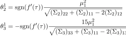
An immediate consequence of Corollary 3 is that, for K > 2, there exists a Gaussian mixture model for which the semi-supervised learning algorithms under study necessarily fail to classify at least one class. To see this, we consider K = 3 and let µ3 = 3µ2 = 6µ1,

C1=C2 =C3,n1=n2=n3,n[l]1=n[l]2 =n[l]3. First, it follows from Corollary 3 that, P(xi → C2|xi ∈ C2)≤P([Gi]2 >[Gi]1|xi ∈ C2) +o(1) = Φ(θ12) +o(1)

P(xi → C3|xi ∈ C3)≤P([Gi]3 >[Gi]1|xi ∈ C3) +o(1) = Φ(θ13) +o(1) Then, under Assumptions 1–2 and the notations of Corollary 3,

θ1₂ = sgn(f0(τ)) µ 2 1

p

(Σ2)22+ (Σ2)11−2(Σ2)12

θ1₃ =−sgn(f0(τ)) 15µ 2 1

p

(Σ3)33+ (Σ3)11−2(Σ3)13

so that f0(τ) <0 ⇒θ1₂ <0,f0(τ)>0⇒θ₃1 <0, while f0(τ) = 0⇒ θ1₂ =θ₃1 = 0. As such, the correct classification rate of elements of C₂ and C₃ cannot be simultaneously greater than 1₂, leading to necessarily inconsistent classifications.

It is nonetheless easy to check that this kind of inconsistency cannot occur ifµ1, µ2 and

0.6 0.8 1

2

√

p

Simulation Corollary 3 Corollary 6

0

.

6

0

.

8

1

2

√ p

Simulation

Corollary 3

Corollary 6

0.6 0.8 1

2

√

p

0

.

6

0

.

8

1

2

√ p

−1.4 −1.3 −1.2 −1.1 −1 −0.9 −0.8 −0.7 −0.6 0.6

0.8 1

2

√

p

α

−

1

.

4

−

1

.

3

−

1

.

2

−

1

.

1

−

1

−

0

.

9

−

0

.

8

−

0

.

7

−

0

.

6

0

.

6

0

.

8

1

2

√ p

α

Figure 3: Theoretical and empirical accuracy as a function of α for 2-class MNIST data (top: digits (0,1), middle: digits (1,7), bottom: digits (8,9)), n= 1024, p= 784,

n_[l]/n= 1/16, n_[u]1 =n_[u]2, Gaussian kernel. Averaged over 50 iterations.

some centered vectors ˜vk=vk−

PK

k0₌₁γ_k0v_k0 wherePK

k0₌₁γ_k0 = 1.2 Inconsistency occurs to

classkif there exista, b6=ksuch that ˜vT_kv˜b >v˜kT˜vk >v˜kTv˜a. To better understand the cause

of this inconsistency, let us consider two extreme scenarios: (i) the vk differ by ‘intensity’,

i.e., vk =rkv fork∈ {1,· · ·, K}, or (ii) thevkdiffer by ‘direction’, i.e,vk=v+uk with

or-thogonaluk’s. In scenario (i), letsmin = argmink∈{1,···,K}rkandsmax= argmaxk∈{1,···,K}rk;

then, fork 6={smin, smax}, min{v˜_kT˜vsmin,˜v

T

kv˜smax} <v˜

T

k˜vk<max{˜vTkv˜smin,v˜

T

kv˜smax} and

in-consistency is thus observed for classesk6={smin, smax}. Contrarily, in scenario (ii), for all 2. The third term of (9) can be seen in this way since for any two symmetric matricesA={aij}mi,j=1andB=

{bij}mi,j=1of same dimensions, trAB=

Pm

i,jaijbij=a T

vbvwithav= [a11,· · ·, a1m,· · ·, am1,· · ·, amm],

k=6 k0 ∈ {1,· · ·, K}, ˜vT_kv˜k≥v˜kTv˜k0 since ˜vT

kv˜k≥0 and ˜vkTv˜k0 ≤0. As such, inconsistency is

less likely to occur if the vk’s have very different directions.

4.2. Choice of f and Suboptimality of the Heat Kernel

As a consequence of the previous section, we shall from here on concentrate on the semi-supervised classification of K= 2 classes. In this case, it is easily seen that,

(K = 2) ∀a6=b∈ {1,2}, kµ˜bk2≥µ˜bTµ˜a, ˜t2b ≥˜ta˜tb, T˜bb≥T˜ab

with equalities respectively for µa = µb, ta = tb, and trCaCb = trCb2. This result, along

with Corollary 3, implies the necessity of the conditions

f0(τ)<0, f00(τ)f(τ)> f0(τ)2, f00(τ)>0

to fully discriminate Gaussian mixtures. As such, from Corollary 3, by letting α = −1, semi-supervised classification of K= 2 classes is always consistent under these conditions.

Since only the first three derivatives off are involved, one may design a simple kernel for any desired values of f0(τ),f00(τ)f(τ)−f0(τ)2 and f00(τ) with a second degree polynomial

f(t) = ax2 +bx+c in such a way that aτ +b = f0(τ), a(aτ2 +bτ +c)−(aτ +b)2 =

f00(τ)f(τ)−f0(τ)2 _{and a=f}00_{(τ), i.e.,}

a=f00(τ) b=f0(τ)−f00(τ)τ c= (f00(τ)f(τ)−f0(τ)τ2)/f00(τ).

Since τ can be consistently estimated in practice by (11) (see the discussion in Subsec-tion 5.1), so cana,b, andc.

A quite surprising outcome of the necessary conditions on the derivatives of f is that the widely used Gaussian (or heat) kernel f(t) = exp(−_2σt2), while fulfilling the condition f0(t) < 0 and f00(t) > 0 for all t (and thus f0(τ) < 0 and f00(τ) > 0), only satisfies

f00(t)f(t) =f0(t)2_{. This indicates that discrimination over t}

1, . . . , tK, under the conditions

of Assumption 1, is asymptotically not possible with a Gaussian kernel. This remark is illustrated in Figure 4 for a discriminative task between two centered isotropic Gaussian classes only differing by the trace of their covariance matrices. There, irrespective of the choice of the bandwidth σ, the Gaussian kernel leads to a constant 1/2 accuracy, where a mere second order polynomial kernel selected upon its derivatives at τ demonstrates good performances. Since p-dimensional isotropic Gaussian vectors tend to concentrate “close to” the surface of a sphere, this thus suggests that Gaussian kernels are not inappropriate to solve the large dimensional generalization of the “concentric spheres” task (for which they are very efficient in small dimensions). In passing, the right-hand side of Figure 4 confirms the need for f00(τ)f(τ)−f0(τ)2 to be positive (there |f0(τ)|<1) as an accuracy lower than 1/2 is obtained for f00(τ)f(τ)−f0(τ)2 <0.

Another interesting fact lies in the choice f0(τ) = 0 (while f00(τ) 6= 0). As already identified by Couillet and Benaych-Georges (2015) and further thoroughly investigated by Couillet and Kammoun (2016), ift1=t2(which can be enforced by normalizing the data set) and ˜Tbb>T˜ba for all a=6 b ∈ {1,2}, then Σb = 0 while [mb]b >[mb]a for allb6=a∈ {1,2}

Gaussian kernel Polynomial kernel of degree 2

f(t) = exp(−_2σt2) f(τ) =f00(τ) = 1

2−5 2−2 21 24 0.5

0.75 1

σ2

−1 0 1

0.5 0.75 1

f00(τ)f(τ)> f0(τ)2

f0(τ)

Figure 4: Empirical accuracy for 2-class Gaussian data with µ1 = µ2, C1 = Ip and C2 = (1 +√3

p)Ip,n= 1024,p= 784,nl/n= 1/16,n[u]1=n[u]2,n[l]1=n[l]2,α =−1.

claimed to ensure a “non-trivial” growth rate regime, asymptotically perfect classification may be achieved by choosing f such that f0(τ) = 0, under the aforementioned statistical conditions. One must nonetheless be careful that thisasymptotic result does not necessarily entail outstanding performances in practical finite dimensional scenarios. Indeed, note that taking f0(τ) = 0 discards the visibility of differing means µ1 6=µ2 (from the expression of [mb]a in Theorem 2); for finite n, p, cancelling the differences in means (often larger than

differences in covariances) may not be compensated for by the reduction in variance. Trials on MNIST particularly emphasize this remark.

4.3. Impact of Class Sizes

A final remark concerns the impact of c_[l] and c0 on the asymptotic performances. Note that c[l] and c0 only act upon the covariance Σb and precisely on its diagonal elements.

Both a reduction inc0 (by increasingn) and an increase inc[l] reduce the diagonal terms in the variance, thereby mechanically increasing the classification performances (if in addition [mb]b>[mb]a fora6=b). In the opposite case of few labeled data, i.e.,c[l]→0, the variance diverges and the performance tends to that of random classification, as shown in Figure 5.

5. Parameter Optimization in Practice

5.1. Estimation of τ

In previous sections, we have emphasized the importance of selecting the kernel functionf

so as to meet specific conditions on its derivatives at the quantity τ. In practice however,

2−10 2−9 2−8 2−7 2−6 2−5 2−4 2−3 2−2 2−1 0.6

0.8 1

Random guess

c[l]

Simulation

Theory (from Corollary 3)

Figure 5: Theoretical and empirical accuracy as a function ofc[l]for 2-class Gaussian data with µ2 = 2µ1 = [6,0,· · ·,0], C1 = Ip and {C2}i,j = .4|i−j|, p = 2048, c0 = 1,

n[u]1=n[u]2,n[l]1=n[l]2,α=−1, Gaussian kernel. Averaged over 50 iterations.

that

ˆ

τ ≡ 1

n(n−1)

n

X

i,j=1 1

pkxi−xjk

2 a.s.

−→τ. (11)

As a consequence, the results of Theorem 2 and subsequently of Corollary 3 hold verbatim with ˆτ in place ofτ. One thus only needs to design f in such as way that its derivatives at ˆ

τ meet the appropriate conditions.

5.2. Optimization of α

In Section 4.2, we have shown that the choice α=−1, along with an appropriate choice of

f, ensures the asymptotic consistency of semi-supervised learning forK = 2 classes, in the sense that non-trivial asymptotic accuracy (>0.5) can be achieved. This choice of α may however not be optimal in general. This subsection is devoted to the optimization of α so as to maximize the average precision, a criterion often used in absence of prior information to favor one class over the other. While not fully able to estimate the optimal α? of α, we shall discuss here a heuristic means to select a close-to-optimalα, subsequently denotedα0.

As per Theorem 2, α must be chosen as α=−1 + √β

p for some β =O(1). In order to

setβ =β? in such a way that the classification accuracy is maximized, Corollary 3 further suggests the need to estimate theθ_baterms which in turn requires the evaluation of a certain number of quantities appearing in the expressions ofmb and Σb. Most of these are however

not directly accessible from simple statistics of the data. Instead, we shall propose here a heuristic and simple method to retrieve a reasonable choice β0 forβ, which we claim is often close to optimal and sufficient for most needs.

To this end, first observe from (9) that the mappingsβ 7→[mb]a satisfy

d

dβ([mb]b−[mb]a) = f0(τ)

f(τ)c[l]

(tb−ta) =−

d

Hence, changes in β induce a simultaneous reduction and increase of either one of [mb]b−

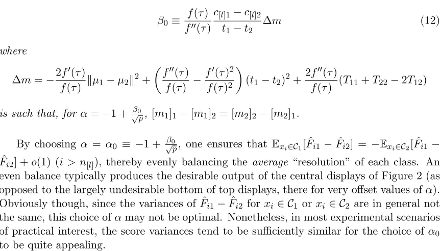
[mb]a and [ma]a−[ma]b. Placing ourselves again in the caseK= 2, we define β0 to be the value for which both differences (witha6=b∈ {1,2}) are the same, leading to the following Proposition–Definition.

Proposition 4 Let K= 2 and [mb]a be given by (9). Then

β0≡

f(τ)

f00_(τ)

c_[l]1−c_[l]2 t1−t2

∆m (12)

where

∆m=−2f

0_(τ)

f(τ) kµ1−µ2k 2₊

f00(τ)

f(τ) −

f0(τ)2

f(τ)2

(t1−t2)2+

2f00(τ)

f(τ) (T11+T22−2T12) is such that, forα=−1 +_√β0

p, [m1]1−[m1]2 = [m2]2−[m2]1.

By choosing α = α0 ≡ −1 + √β0_p, one ensures that Exi∈C1[ ˆFi1−Fˆi2] = −Exi∈C2[ ˆFi1−

ˆ

Fi2] +o(1) (i > n[l]), thereby evenly balancing the average “resolution” of each class. An even balance typically produces the desirable output of the central displays of Figure 2 (as opposed to the largely undesirable bottom of top displays, there for very offset values ofα). Obviously though, since the variances of ˆFi1−Fˆi2 forxi ∈ C1 orxi ∈ C2 are in general not the same, this choice ofαmay not be optimal. Nonetheless, in most experimental scenarios of practical interest, the score variances tend to be sufficiently similar for the choice ofα0 to be quite appealing.

This heuristic motivation made, note thatβ0is proportional toc[l]b−c[l]a. This indicates

that the more unbalanced is the labelled data set, the more deviated from zero is β0. In particular, for n_[l]1 =n_[l]2,α0 =−1. As we shall subsequently observe in simulations, this remark is of dramatic importance in practice where takingα=−1 (the PageRank method) in place of α=α0 leads to significant performance losses.

Of utmost importance here is the fact that, unlikeθa_b which are difficult to assess empir-ically, a consistent estimate of β0 can be obtained through a rather simple method, which we presently elaborate on.

While an estimate fortaandTabcan be obtained empirically from the labelled data

them-selves,kµ1−µ2k2is not directly accessible (note indeed that _n1

[l]a P

Caxi =µa+

1

n[l]a P

Cawi,

for some wi ∼ N(0, Ca), and the central limit theorem guarantees that k_n1

[l]a P

Cawik = O(1), the same order of magnitude as kµa−µbk). However, one may access an estimate

for ∆m by running two instances of the PageRank algorithm (α = −1), resulting in the method described in Algorithm 1. It is easily shown that, under Assumptions 1–2,

ˆ

β0−β0 a.s.

−→0.

Algorithm 1 Estimate ˆβ0 of β0. 1: Let ˆτ be given by (11). 2: Let

c

∆t= 1 2√p



 Pn[l]1

i,j=1kxi−xjk2

n[l]1(n[l]1−1)

− Pn[l]

i,j=n[l]1+1kxi−xjk

2

n[l]2(n[l]2−1)





3: Setα=−1 and define J ≡pPn

i=n[l]+1

ˆ

Fi1−Fˆi2.

4: Still for α =−1, reduce the set of labelled data to n0_[l]1 = n_[0_l]2 = min{n[l]1, n[l]2} and, with obvious notations, letJ0 ≡pPn

i=n0_[l]+1Fˆ

0

i1−Fˆi02. 5: Return ˆβ0≡

c[l]f(ˆτ)

f0_(ˆτ)

c

∆t J0_−J

n[u] .

snapshots of typical classification precision obtained from examples of n = 4096 images with c[l] = 1/16. As expected, the gain in performance is largest as |c[l]1−c[l]2| is large. More surprisingly, the performances obtained are impressively close to optimal. It should be noted though that simulations revealed more unstable estimates of ˆβ0 for smaller values of n.

Note that the method for estimating β0 provided in Algorithm 1 implicitly exploits the resolution of two equations (through the observation of J, J0 obtained for different values of n_[l]1, n_[l]2) to retrieve the value of ∆m defined in Proposition 4. Having access to ∆m further allows access to kµ1 −µ2k2, for instance by setting f so that f00(τ) = 0 and f00(τ)f(τ) = f0(τ)2. This in turn allows access to all terms intervening in [mb]a (as

per (9)), making it possible to choose f so to maximize the distances |[m1]1−[m1]2| and

|[m2]2−[m2]1|. However, in addition to the cumbersome aspect of the induced procedure (and the instability implied by multiple evaluations of the scores F under several settings forf and c[l]a), such operations also alter the values of the variances in (10) for which not

all terms are easily estimated. It thus seems more delicate to derive a simple method to optimizef in addition toα.

6. Concluding Remarks

This article is part of a series of works consisting in evaluating the performance of kernel-based machine learning methods in the large dimensional data regime (Couillet and Benaych-Georges, 2015; Liao and Couillet, 2017; Couillet and Kammoun, 2016). Relying on the derivations of Couillet and Benaych-Georges (2015) that provide a Taylor expansion of ra-dial kernel matrices around the limiting common value τ of 1_pkxi −xjk2 for i 6= j and

0.9 0.92 0.94 0.96 0.98 1

α=α?_(oracle)

α=−1 +_√βˆ0

p (Algorithm 1)

α=−1 (PageRank method)

0.8 0.85 0.9 0.95 1

2−4 2−3 2−2 2−1

0.8 0.85 0.9 0.95 1

c[l]1

Figure 6: Average precision varying with c_[l]1 for 2-class MNIST data (top: digits (0,1), middle: digits (1,7), bottom: digits (8,9)), n= 4096, p = 784, n[l]/n= 1/16,

n[u]1=n[u]2, Gaussian kernel.

expression at the core of the limiting performance assumes a different form. Of importance is the finding that, under a heat kernel assumption f(t) = exp(− t

2σ2), the studied

semi-supervised learning method fails to classify Gaussian mixtures of the type N(0, Ck) with

trC_k◦ =O(√p) and trCkCk0 −trC2

k = o(p), which unsupervised learning or LS-SVM are

able to do (Couillet and Benaych-Georges, 2015; Liao and Couillet, 2017). This paradox may deserve a more structural way of considering together methods on the spectrum from unsupervised to supervised learning.

The very fact that the kernel matrix W is essentially equivalent to the matrixf(τ)1n1Tn

natural behavior of kernels, essentially follows from the Gaussian mixture model we assumed as well as from the decision to compare vectors by means of a mere Euclidean distance. We believe that this simplistic (although widely used) method explains the strong coincidence between performances on the Gaussian mixture model and on real data sets. Indeed, as radial functions are not specially adapted to image vectors (as would be wavelet or convolu-tional filters), the kernel likely operates on first order statistics of the input vectors, hence similar to its action on a Gaussian-mixture data. It would be interesting to generalize our result, and for that matter the set of works (Couillet and Benaych-Georges, 2015; Liao and Couillet, 2017; Couillet and Kammoun, 2016), to more involved data-oriented kernels, so long that the data contain enough exploitable degrees of freedom.

It is also quite instructive to note that, from the proof of our main results, the terms re-maining after the expansion ofD−_[u1_]−αW_[uu]Dα_[u]appearing in (2) almost all vanish, strongly suggesting that similar results would be obtained if the inverse matrix in (2) were dis-carded altogether. This implies that the intra-unlabelled data kernel W_[uu] is of virtually no asymptotic use. Also, the remark of Section 4.3 according to which c[l] → 0 implies a vanishing classification rate suggests that even the (unsupervised) clustering performance obtained by Couillet and Benaych-Georges (2015) is not achieved, despite the presence of possibly numerous unlabelled data. This, we believe, is due to a mismatched scaling in the SSL problem definition. A promising avenue of investigation would consist in introducing appropriate scaling parameters in the label propagation method or the optimization (1) to ensure that W[uu] is effectively used in the algorithm. Early simulations do suggest that elementary amendments to (2) indeed result in possibly striking performance improvements.

These considerations are left to future works.

Acknowledgments

This work is supported by the ANR Project RMT4GRAPH (ANR-14-CE28-0006).

Appendix A. Preliminaries

We begin with some additional notations that will be useful in the proofs.

• Forxi∈ Ck,ωi ≡(xi−µk)/

√

p, and Ω≡[ω1,· · · , ωn]T

• jk∈Rn is the canonical vector of Ck, in the sense that its i-th element is 1 ifxi∈ Ck

or 0 otherwise. j_[l]k and j_[u]k are respectively the canonical vectors for labelled and unlabelled data ofCk.

• ψi≡ kωik2−E[kωik2],ψ≡[ψ1,· · ·, ψn]T and (ψ)2 ≡[(ψ1)2,· · · ,(ψn)2]T.

Theorem 5 Forxi ∈ Cb an unlabelled vector (i.e., i > n[l]), letFˆia be given by (7) withF

defined in (2)for α =O(1). Then, under Assumptions 1–2,

pFˆi·=p(1 +zi)1K+Gi+oP(1)

Gi∼ N(mb,Σb)

where zi is as in Theorem 2 and

(i) for Fi· considered on the σ-field induced by the random variables x[l]+1, . . . , xn, p =

1,2, . . .,

[mb]a=Hab+

1

n[l]

K

X

d=1

(αnd+n[u]d)Had

+ (1 +α) n

n[l]

"

∆a+

p n[l]a

f0(τ)

f(τ)ψ

T

[l]j[l]a−α

f0(τ)2

f(τ)2tatb

#

(13)

[Σb]a1a2 =

(−α2−α)n−n[l]

n[l]

f0(τ)2

f(τ)2 +

f00(τ)

f(τ)

!2

Tbbta1ta2

+δa2

a1 f0(τ)2

f(τ)2

4c0Tba1 c[l]a1

+4f

0_(τ)2

f(τ)2 µ

◦ a1Cbµ

◦

a2 (14)

where

Hab=

f0(τ)

f(τ)kµ

◦

b−µ

◦ ak2+

f00(τ)

f(τ) −

f0(τ)2

f(τ)2

tatb+

2f00(τ)

f(τ) Tab (15)

∆a=

√ pf0(τ)

f(τ) ta+

αf0(τ)2+f(τ)f00(τ)

2f(τ)2 2Taa+t 2

a

+ 1

n[l]

f0(τ)

f(τ)

2 K

X

d=1

n_[u]dtd

!

ta.

(16)

(ii) for Fi· considered on theσ-field induced by the random variables x1, . . . , xn,

[mb]a=Hab+

1

n_[l]

K

X

d=1

(αnd+n[u]d)Had+ (1 +α)

n n_[l]

"

∆a−α

f0(τ)2

f(τ)2tatb

#

[Σb]a1a2 =

(−α2−α)n−n[l]

n[l]

f0(τ)2

f(τ)2 +

f00(τ)

f(τ)

!2

Tbbta1ta2

+δa2

a1 f0(τ)2

f(τ)2

(1 +α)2

c2_[l]

2c0Taa

c[l]a1

+4c0Tba1 c[l]a1

!

+ 4f

0_(τ)2

f(τ)2 µ

◦ a1Cbµ

◦ a2

withHab given in (15) and ∆a in (16).

probability. Recall that the probability of correct classification ofxi ∈ Cb is the same as the

probability of ˆFib >maxa6=bFˆib, which, according to the above theorem, is asymptotically

the probability that [Gi]b is the greatest element ofGi. Particularly forK = 2, we have the

following corollary.

Corollary 6 Under the conditions of Theorem 1, and with K = 2, we have, for a 6=b ∈ {1,2},

(i) Conditionally on x1,· · · , xn[l],

P

xi → Cb|xi∈ Cb, x1,· · · , xn[l])−Φ(θ

a b

→0

θ_ba= p [mb]b−[mb]a

[Σb]bb+ [Σb]aa−2[Σb]ab

where Φ(u) = ₂1_πRu

−∞exp(−t2/2)dt and mb, Σb are given in (i) of Theorem 5.

(ii) Unconditionally,

P(xi → Cb|xi ∈ Cb)−Φ(θba)→0

θ_ba= p [mb]b−[mb]a

[Σb]bb+ [Σb]aa−2[Σb]ab

where heremb, Σb are given in (ii) of Theorem 5.

The remainder of the appendix is dedicated to the proof of Theorem 5 and Corollary 6 from which the results of Section 3.2 directly unfold.

Appendix B. Proof of Theorems 5

The proof of Theorem 5 is divided into two steps: first, we Taylor-expand the normalized scores for unlabelled data ˆF_[u] using the convergence 1_pkxi −xjk2 a

.s.

−→τ for all i 6= j; this

expansion yields a random equivalent ˆF_[eq_u]in the sense thatp( ˆF[u]−Fˆ_[eq_u]) a.s.

−→0. Proposition 1

is directly obtained from ˆF_[eq_u]. We then complete the proof by demonstrating the convergence to Gaussian variables of ˆF_[eq_u] by means of a central limit theorem argument.

B.1. Step 1: Taylor expansion

In the following, we provide a sketch of the development ofF_[u]; most unshown intermediary steps can be retrieved from simple, yet painstaking algebraic calculus.

Recall from (2) the expression of the unnormalized scores for unlabelled data

F_[u]= (Inu−D

−1−α

[u] W[uu]Dα[u])

−1_D−1−α

[u] W[ul]D[αl]F[l].

for all i 6= j, we first Taylor-expand Wij = f(kxi −xjk2/p) around f(τ) to obtain the

following expansion forW, already evaluated by Couillet and Benaych-Georges (2015),

W =W(n)+W(

√

n)_+W(1)_+O(n−1

2) (17)

wherekW(n)k=O(n),kW(

√

n)_=O(√_{n) and kW}(1)_{k=O(1), with the definitions}

W(n)=f(τ)1n1Tn

W(

√ n)_=f0

(τ)

"

ψ1T_n+ 1nψT+ K

X

b=1

tb

√ pjb

!

1T_n+ 1n K X a=1 ta √ pj T a #

W(1)=f0(τ)

" _K X

a,b=1

kµ◦_a−µ◦_bk2

p jbj

T a − 2 √ pΩ K X a=1

µ◦_aj_aT+√2 p

K

X

b=1

diag(jb)Ωµ◦b1Tn

−√2 p

K

X

b=1

jbµ◦bTΩT+

2

√ p1n

K

X

a=1

µ◦_aTΩTdiag(ja)−2ΩΩT

#

+f

00_(τ)

2

(ψ)21T_n+ 1n[(ψ)2]T+ K

X

b=1

t2_b pjb1

T

n+ 1n K

X

a=1

t2_a pj T a + 2 K X a,b=1

tatb

p jbj

T

a + 2

K

X

b=1

diag(jb)

tb

√ pψ1

T

n+ 2

K

X

b=1

tb

√ pjbψ

T_{+ 2}

K

X

a=1

1nψTdiag(ja)

ta

√ p

+ 2ψ

K X a=1 ta √ pj T

a + 4

K

X

a,b=1

Tab

p jbj

T

a + 2ψψT

+ (f(0)−f(τ) +τ f0(τ))In.

As W_[ul], W_[uu] are sub-matrices of W, their approximated expressions are obtained directly by extracting the corresponding subsets of (17). Applying then (17) in D = diag(W1n), we next find

D=nf(τ)

In+

1

nf(τ)diag(W (√n)₁

n+W(1)1n)

+O(n−12).

Thus, for anyσ∈_R, (n−1D)σ can be Taylor-expanded aroundf(τ)σIn as

(n−1D)σ =f(τ)σ

In+

σ1

nf(τ)diag((W

(√n)_+W(1)₎₁

n) +

σ(σ−1) 2n2_f(τ)2diag

2_(W(√n)₁

n)

+O(n−32) (18)

where diag2(·) stands for the squared diagonal matrix. The Taylor-expansions of (n−1D[u])α and (n−1D[l])α are then directly extracted from this expression forσ =α, and similarly for (n−1D_[u])−1−α withσ=−1−α. Since

D−_[u1_]−αW_[ul]D_[α_l]= 1

n(n

−1_D

[u])−1−αW[ul](n−1D[l])α

it then suffices to multiply the Taylor-expansions of (n−1D_[u])α, (n−1D_[l])α, andW_[ul], given respectively in (18) and (17), normalize bynand then organize the result in terms of order

The term D−_[u1_]−αW_[uu]Dα_[u]is dealt with in the same way. In particular,

D_[−_u1_]−αW[uu]D[αu]= 1

n1n[u]1n[l]+O(n

−1 2).

Therefore, (In[u]−D

−1−α

[u] W[uu]Dα[u])

−1 _{may be simply written as}

In[u]−

1

n1n[u]1n[u]+O(n

−1 2)

−1

=In[u]+

1

n[l]

1n[u]1n[u]+O(n

−1 2).

Combining all terms together completes the full linearization of ˆF[u].

This last derivation, which we do not provide in full here, is simpler than it appears and is in fact quite instructive in the overall behavior of F[u]. Indeed, only product terms in the development of (In[u]−D

−1−α

[u] W[uu]D

α

[u])

−1 _{and D}−1−α

[u] W[ul]D

α

[l]F[l] of order at least

O(1) shall remain, which discards already a few terms. Now, in addition, note that for any vector v, v1T_n[l]F[l] = v1T_k so that such matrices are non informative for classification (they have identical score columns); these terms are all placed in the intermediary variable

z, the entries zi of which are irrelevant and thus left as is (these are the zi’s of

Proposi-tion 1 and Theorem 2). It is in particular noteworthy to see that all terms of W_[(1)_uu] that remain after taking the product with D−_[u1_]−αW_[ul]D_[α_l]F[l] are precisely those multiplied by

f(τ)1n[u]1

T

n[l]F

[l] _{and thus become part of the vectorz. Since most informative terms in the} kernel matrix development are found in W(1), this means that the algorithm under study shall make little use of theunsupervisedinformation about the data (those found inW_[(1)_uu]). This is an important remark which, as discussed in Section 6, opens up the path to further improvements of the semi-supervised learning algorithms which would use more efficiently the information in W_[(1)_uu].

All calculus made, this development finally leads toF_[u]=F_[eq_u]with, fora, b∈ {1, . . . , K}

and xi ∈ Cb,i > n[l], ˆ

F_iaeq= 1 +1

p "

Hab+

1

n_[l]

K

X

d=1

Had(αnd+n[u]d)

#

+ (1 +α) n

pn_[l] "

∆a−α

f0(τ)2

f(τ)2tatb

#

+ (−α

2_−α)n−n [l]

n[l]

f0(τ)2

f(τ)2 +

f00(τ)

f(τ)

! ta

√ pψi+

2f0(τ)

f(τ)√pµ

◦ aωi

+f

0_(τ)

f(τ)

(1 +α)n n[l]n[l]a

ψ_[T_l]j[l]a+

4

n[l]a

j_[T_l]aΩ[l]ωi

!

+zi (19)

where Hab is as specified in (15), ∆a as in (16), and zi =O(

√

p) is some residual random variable only dependent on xi. Gathering the terms in successive orders of magnitude,

Proposition 1 is then straightforwardly proven from (19).

B.2. Step 2: Central limit theorem

The focus of this step is to examineGi =p( ˆF_ieq−(1 +zi)1K). Theorem 5 can be proven by

First consider Item (i) of Theorem 5, which describes the behavior of ˆF_[u]conditioned on

x1, . . . , xn[l]. Recall that a necessary and sufficient condition for a vectorv to be a Gaussian

vector is that all linear combinations of the elements ofv are Gaussian variables. Thus, for given x1, . . . , xn[l] deterministic, according to (19), Gi is asymptotically Gaussian if, for all g1∈R,g2∈Rp,g1ψi+g2Tωi has a central limit.

Letting ωi = C

1 2 b

√

pr, with r ∼ N(0, Ip), g1ψi+g2ωi can be rewritten as rTAr+br+c

with A=g1C_pb,b=g2C_pb,c=−g1tr_pCb. SinceA is symmetric, there exists an orthonormal matrixU and a diagonal Λ such thatA=UTΛU. We thus get

rTAr+br+c=rTUTΛU r+bUTU r+c= ˜rTΛ˜r+ ˜br˜+c

with ˜r=U rand ˜b=bUT. By unitary invariance, we have ˜r∼ N(0, Ip) so thatg1ψi+g2ωiis

thus the sum of the independent but not identically distributed random variablesqj =λjr˜j2+

˜_{bj˜rj,i= 1, . . . , p. From Lyapunov’s central limit theorem (Billingsley, 1995, Theorem 27.3),}

it remains to find aδ >0 such that

P

jE|qj−E[qj]|2+δ

(P

jVar[qj])

1+δ/2 →0 to ensure the central limit theorem.

For δ = 1, we have E[qj] = λj, Var[qj] = 2λ2_j + ˜b2_j and E(qj−E[qj])3

= 8λ3_j + 6λj˜b2_j, so

that

P

jE[|qj−E[qj]|3]

(P

jVar[qj])

3/2 =O(n

−1 2).

It thus remains to evaluate the expectation and covariance matrix ofG_i conditioned on

x1, . . . , xn[l] to obtain (i) of Theorem 5. For xi∈ Cb, we have

E{[Gi]a}=Hab+

1

n_[l]

K

X

d=1

(αnd+n[u]d)Had

+ (1 +α) n

n[l]

"

∆a+

p n[l]a

f0(τ)

f(τ)ψ

T

[l]j[l]a−α

f0(τ)2

f(τ)2tatb

#

Cov{[Gi]a1[Gi]a2}=

(−α2−α)n−n[l]

n[l]

f0(τ)2

f(τ)2 +

f00(τ)

f(τ)

!2

Tbbta1ta2

+δa2

a1 f0(τ)2

f(τ)2

4c0Tba1 c[l]a1

+4f

0_(τ)2

f(τ)2 µ

◦ a1Cbµ

◦

a2+o(1).

From the above equations, we retrieve the asymptotic expressions of [mb]a and [∆b]a1a2

given in (13) and (14). This completes the proof of Item (i) of Theorem 5. Item (ii) is easily proved by following the same reasoning.

References

Konstantin Avrachenkov, Paulo Gon¸calves, Alexey Mishenin, and Marina Sokol. Gener-alized optimization framework for graph-based semi-supervised learning. arXiv preprint arXiv:1110.4278, 2011.

Mikhail Belkin and Partha Niyogi. Semi-supervised learning on riemannian manifolds. Machine learning, 56(1-3):209–239, 2004.

Mikhail Belkin, Irina Matveeva, and Partha Niyogi. Regularization and semi-supervised learning on large graphs. InInternational Conference on Computational Learning Theory (COLT), pages 624–638. Springer, 2004.

Peter J Bickel, Bo Li, et al. Local polynomial regression on unknown manifolds. InComplex Datasets and Inverse Problems, pages 177–186. Institute of Mathematical Statistics, 2007.

P. Billingsley. Probability and Measure. John Wiley and Sons, Inc., Hoboken, NJ, third edition, 1995.

Olivier Chapelle, Bernhard Sch¨olkopf, and Alexander Zien. Semi-Supervised Learning. MIT press, 2006.

Romain Couillet and Florent Benaych-Georges. Kernel spectral clustering of large dimen-sional data. arXiv preprint arXiv:1510.03547, 2015.

Romain Couillet and Abla Kammoun. Random matrix improved subspace clustering. In Asilomar Conference on Signals, Systems and Computers, pages 90–94. IEEE, 2016.

Akshay Gadde, Aamir Anis, and Antonio Ortega. Active semi-supervised learning using sampling theory for graph signals. In International Conference on Knowledge Discovery and Data Mining, pages 492–501. ACM, 2014.

Amir Globerson, Roi Livni, and Shai Shalev-Shwartz. Effective semi-supervised learning on manifolds. InInternational Conference on Learning Theory (COLT), pages 978–1003, 2017.

Andrew B Goldberg, Xiaojin Zhu, Aarti Singh, Zhiting Xu, and Robert Nowak. Multi-manifold semi-supervised learning. 2009.

Martin Szummer Tommi Jaakkola and Martin Szummer. Partially labeled classification with markov random walks. International Conference in Neural Information Processing Systems, 14:945–952, 2002.

Thorsten Joachims et al. Transductive learning via spectral graph partitioning. In Inter-national Conference on Machine Learning, volume 3, pages 290–297, 2003.

Yann LeCun, Corinna Cortes, and Christopher JC Burges. The mnist database of hand-written digits, 1998.

Amit Moscovich, Ariel Jaffe, and Boaz Nadler. Minimax-optimal semi-supervised regression on unknown manifolds. arXiv preprint arXiv:1611.02221, 2016.

Boaz Nadler, Nathan Srebro, and Xueyuan Zhou. Semi-supervised learning with the graph laplacian: the limit of infinite unlabelled data. In International Conference on Neural Information Processing Systems, pages 1330–1338, 2009.

Sunil K Narang, Akshay Gadde, and Antonio Ortega. Signal processing techniques for interpolation in graph structured data. In IEEE International Conference Acoustics, Speech and Signal Processing, pages 5445–5449. IEEE, 2013a.

Sunil K Narang, Akshay Gadde, Eduard Sanou, and Antonio Ortega. Localized iterative methods for interpolation in graph structured data. In Global Conference on Signal and Information Processing, pages 491–494. IEEE, 2013b.

Bernhard Sch¨olkopf and Alexander J Smola. Learning with Kernels: Support Vector Ma-chines, Regularization, Optimization, and Beyond. MIT press, 2002.

Larry Wasserman and John D Lafferty. Statistical analysis of semi-supervised regression. In International Conference on Neural Information Processing Systems, pages 801–808, 2008.

Dengyong Zhou, Olivier Bousquet, Thomas Navin Lal, Jason Weston, and Bernhard Sch¨olkopf. Learning with local and global consistency. volume 16, pages 321–328, 2004.

Xiaojin Zhu and Zoubin Ghahramani. Learning from labeled and unlabeled data with label propagation. Technical report, Citeseer, 2002.