Interleave Variational Optimization with Monte Carlo Sampling: A Tale of Two Approximate Inference Paradigms

(1)

The Thirty-Third AAAI Conference on Artificial Intelligence (AAAI-19)

Interleave Variational Optimization with Monte

Carlo Sampling: A Tale of Two Approximate Inference Paradigms

Qi Lou

University of California, Irvine Irvine, CA 92697, USA

[email protected]

Rina Dechter

[email protected]

Alexander Ihler

[email protected]

Abstract

Computing the partition function of a graphical model is a fundamental task in probabilistic inference. Variational bounds and Monte Carlo methods, two important approxi-mate paradigms for this task, each has its respective strengths for solving different types of problems, but it is often non-trivial to decide which one to apply to a particular problem instance without significant prior knowledge and a high level of expertise. In this paper, we propose a general framework that interleaves optimization of variational bounds (via mes-sage passing) with Monte Carlo sampling. Our adaptive inter-leaving policy can automatically balance the computational effort between these two schemes in an instance-dependent way, which provides our framework with the strengths of both schemes, leads to tighter anytime bounds and an unbiased estimate of the partition function, and allows flexible trade-offs between memory, time, and solution quality. We verify our approach empirically on real-world problems taken from recent UAI inference competitions.

Introduction

Probabilistic graphical models, including Bayesian networks and Markov random fields, are a set of powerful frame-works for representing and reasoning with probabilistic and deterministic information (Darwiche 2009; Dechter 2013; Dechter, Geffner, and Halpern 2010). Reasoning in a graph-ical model often requires computing the partition function, i.e., the normalizing constant of the underlying distribution. Exact computation of the partition function is known to be intractable (Valiant 1979) in general, leading to the develop-ment of many approximate schemes, the major categories of which are variational methods, Monte Carlo sampling, and search algorithms. Within these, techniques that provide some guaranteed confidence intervals on the correct value, and can be improved with additional computation, are valued for providing users with concrete information or certificates of accuracy within a reasonable amount of time, and allowing the user to decide the desired balance of quality versus time. Variational bounds (Wainwright and Jordan 2008) and closely related approximate elimination methods (Dechter and Rish 2003; Liu and Ihler 2011) provide deterministic guarantees on the partition function. However, these bounds

are not anytime; their quality often depends critically on the amount of memory available, and do not continue to improve (approach the correct value) without additional memory.

Monte Carlo methods (Liu 2008), such as importance sam-pling (Dagum and Luby 1997; Liu, Fisher, and Ihler 2015) gives probabilistic bounds that improve with more samples at a predictable rate; in practice this means bounds that improve rapidly at first, but can be slow to become very tight.

Search algorithms (Henrion 1991; Viricel et al. 2016; Lou, Dechter, and Ihler 2017a) explicitly enumerate over the space of configurations and eventually provide an exact answer; however, while some problems are well-suited to search, others only improve their quality very slowly with more computation.

Several algorithms combine two or more strategies. Ap-proximate hash-based counting combines sampling (of hash functions) with CSP-based search (Chakraborty et al. 2014; Chakraborty, Meel, and Vardi 2016) or other MAP queries (Ermon et al. 2013; 2014), although these are not typ-ically formulated to provide anytime behavior. Some recent works combine importance sampling with (partially) exact inference (Broka et al. 2018; Friedman and Van den Broeck 2018), though they do not have guarantees on their estimates. A number of works use some form of approximate elimina-tion or variaelimina-tional bounds as search heuristics, such as Lou, Dechter, and Ihler (2017a), while Liu, Fisher, and Ihler (2015) develops an importance sampling proposal from variational bounds that provides strong probabilistic confidence intervals. More recently, Lou, Dechter, and Ihler (2017b) unifies these two works within the same framework.

(2)

opti-mization of variational bounds with importance sampling from the very beginning, and provides an instance-specific balance designed to give rapid anytime improvement.

Our contributions. First, we propose a general framework that interleaves optimization of variational upper bounds with importance sampling to achieve anytime upper and lower bounds of the partition function, which is directly applicable to a set of convex variational bounds including TRW (Wain-wright, Jaakkola, and Willsky 2005) and WMB (Liu and Ihler 2011). Second, we propose an effective adaptive policy that automatically balances the computational effort between these two processes on the fly in a problem-dependent fashion. Third, our experiments on real-world problems demonstrate that our interleaving framework with the adaptive policy is superior to several non-interleaving baselines and interleav-ing baselines with simple static policies in terms of anytime performance, gives competitive final bound quality, and is relatively insensitive to its hyperparameter, making it easy to use and automate in practice.

Background

In this section, we introduce some notations and background knowledge that are essential to present and understand our algorithm.

LetX = (X1, . . . , Xn)be a vector of random variables,

where eachXitakes values in a discrete domainXi; we use

lower case letters, e.g.xi∈ Xi, to indicate a value ofXi, and

xto indicate an assignment ofX. A graphical model overX

consists of a set of factorsF ={fα(Xα)|α∈ I}, where

each factorfαis defined on a subsetXα={Xi |i∈α}of

X, called its scope.

We associate an undirected graphG = (V, E)with F,

where each nodei∈V corresponds to a variableXiand we

connect two nodes,(i, j) ∈ E, iff{i, j} ⊆ αfor someα. The setIthen corresponds to cliques ofG. We can interpret

Fas an unnormalized probability measure, so that

f(x) = Y

α∈I

fα(xα), Z =

X

x

Y

α∈I

fα(xα).

Zis called thepartition function, and normalizesf(x).

Com-putingZ is often a key task in evaluating the probability

of observed data, model selection, or computing predictive probabilities.

Weighted Mini-bucket

In experiments, we apply our framework to a particular varia-tional bound called weighted mini-bucket (WMB) (Liu and Ihler 2011), which we briefly introduce here to make our paper self-contained. WMB is an approximate elimination algorithm that generalizes its elimination-based predeces-sors (e.g., bucket elimination (Dechter 1999), mini-bucket elimination (Dechter and Rish 2003)) by relaxing the exact summation using a “power sum” operation during variable elimination, and controls the computational complexity using a user-specified parameter called theibound.

Given an elimination order, WMB processes variables one by one. Upon reaching a variable, say,Xi, WMB first collects

all factors (including those intermediately generated ones,

termed “messages”) withXiin their scopes, which form a

factor set called “bucket”Bi. WMB then partitionsBiinto

several disjoint “mini-buckets”{B_ij}to ensure that eachB_ij

involves no more than (ibound+ 1) variables.

After assigning a “weight”ρij to eachB

j

i, WMB

elimi-natesXiin factors ofB j

i using the power sum:

λi→πij = (

X

xi

Y

fα∈Bij f

1

ρij

α )ρij,

which sends a messageλi→πij toXπij, the earliest unelimi-nated variable in the scope ofλi→πij. This messageλi→πij is then placed in the bucket ofXπij for later processing.

When the weightsρij’s are nonnegative and sum to one,

H¨older’s inequality guarantees that the product of the mes-sagesλi→πij is an upper bound of the sum, i.e.,

X

xi

Y

fα∈Bi fα≤

Y

j

λi→πij.

Therefore, WMB eventually returns an upper boundUof the

partition functionZafter it terminates. Liu and Ihler (2011) also shows that the resulting bound is equivalent to a class of bounds based on tree reweighted (TRW) belief propa-gation (Wainwright, Jaakkola, and Willsky 2005), or more generally conditional entropy decompositions (Globerson and Jaakkola 2007).

U can be tightened by cost shifting (a.k.a., reparameteri-zation) and weight optimization, which can be implemented in a forward-backward message passing procedure. We refer readers to Liu and Ihler (2011) for details.

Weighted Mini-bucket Importance Sampling

This same relaxation of WMB can also be used to define a proposal distributionq(x)(Liu, Fisher, and Ihler 2015) as follows:

q(x) =Y

i

X

j

ρijqij(xi|xanj(i)), (1)

whereXanj(i)are variables included in the mini-bucketB

j i

excludingXi. Theqij(xi|xanj(i))’s are conditional distribu-tions:

qij(xi|xanj(i)) =

Y

fα∈Bji

fα/λi→πij

_ρij1 .

One can show that importance weights derived from this proposal distribution are bounded and unbiased, i.e.,

f(x)/q(x)≤U, _E

f(x)/q(x)

=Z, (2)

which leads to finite-sample bounds of the partition function (see Corollary 3.2 of Liu, Fisher, and Ihler (2015)).

Example. Fig. 1 shows an example of running WMB on a pairwise graphical model to produce an upper bound of the partition function and a proposal distribution when an

(3)

A" B"

C" D"

E" F"

G"

(a)

A

f(A,B) B

f(B,C)

C F f(B,F)

f(A,G) f(F,G) G f(B,E) f(C,E) E f(B,D) f(C,D) D

λF_(A,B) λB_(A)

λE_(B,C) λD_(B,C)

λC_(B) λD_(A)

f(A,D) D

mini-buckets

λG_(A,F)

f(A)

U

(b)

...

(c)

Figure 1: (a) A graphical model over 7 variables. (b) Given an elimination orderG, F, E, D, C, B, A, andibound= 2, WMB

runs on this model to produce an upper bound of the partition function. (c) The same relaxation from (b) gives a proposal distribution with properties present in (2).

Interleaving Variational Optimization with

Importance Sampling

In this section, we present a general scheme that interleaves optimization of the variational upper bound with importance sampling, derive finite-sample bounds for this scheme, and discuss interleaving policies.

A General Interleaving Framework

Our general scheme is quite simple: we interleave the two processes according to some policy. Since optimization of variational bounds is typically through a message passing procedure, we consider interleaving message passing with importance sampling in our algorithm. Procedurally, we first build up an initial bound within a given memory budget, and then interleave the two processes following a policy that we will discuss in the sequel. Alg. 1 presents details of our framework.

Our framework actually serves as a “meta-algorithm” from which any optimizable proposal with properties in (2) can benefit; in particular this includes convex variational bounds such as WMB and TRW (see Liu, Fisher, and Ihler (2015) for more details on why this holds for TRW).

Interleaving these two processes leads to rapid early bound improvement, since the improvement provided by the proba-bilistic bounds is not delayed until after variational optimiza-tion converges or is otherwise terminated (e.g., in Liu, Fisher, and Ihler (2015) and Lou, Dechter, and Ihler (2017b)); this results in significant improvements in anytime behavior as we demonstrate in the empirical evaluation. A critical point is that, by interleaving updates to the proposal, our samples are no longer identically distributed; in fact, their variance is decreasing as the proposal improves, and for best results we should up-weight these more accurate samples in our es-timates. To this end, and analogous to that of Lou, Dechter, and Ihler (2017b), we define a weighted average estimatorZˆ

and apply an empirical Bernstein bound (Maurer and Pontil 2009) to derive finite-sample bounds on the error between

ZandZˆbased on independent samples from a sequence of

proposals satisfying (2):

Algorithm 1A General Interleaving Framework

Require: memory budget, time budget, confidence parame-terδ, interleaving policyP.

Ensure: N,U,Zb,HM(U),∆,Vard.

1: Build an initial variational upper bound that fits the mem-ory budget.

2: whilewithin the time budgetdo

3: Generate(R, S)via policyP.

4: forr←1toRdo

5: Run one round of message passing.

6: UpdateU.

7: end for

8: fors←1toSdo

9: Draw one sample from the current proposal.

10: UpdateN,Zb,HM(U),∆,Vardvia (3), (4), (6)

11: and (7) respectively.

12: end for

13: Update policyPif necessary.

14: end while

Theorem 1. Let{xi_}N

i=1be a series of samples drawn from

proposal distributions {qi(x)}Ni=1 respectively via Alg. 1,

with{Zbi=f(xi)/qi(xi)}Ni=1the corresponding importance

weights, and{Ui}Ni=1 the corresponding variational upper

bounds respectively. Let

b

Z= HM(U)

N

X

i=1 b Zi

Ui

, (3)

where

HM(U) =h1

N

X

i=1

1

Ui

i−1

(4)

is the harmonic mean of{Ui}Ni=1. then, Zb is an unbiased

estimator ofZ, i.e.,

(4)

Define a deviation term

∆ = HM(U)

s

2Var ln(2d /δ)

N +

7 ln(2/δ) 3(N−1)

, (6)

where

d

Var = 1

N−1

N

X

i=1 h bZi

Ui

− Zb

HM(U)

i2

(7)

is the unbiased empirical variance of{Zbi/Ui}Ni=1. Since the

boundedness of eachZbiguarantees thatZbi/Ui≤1for alli,

applying standard empirical Bernstein results we have

Pr[Z ≤Zb+ ∆]≥1−δ,

Pr[Z ≥Zb−∆]≥1−δ,

(8)

i.e.,Zb+ ∆andZb−∆are upper and lower bounds ofZwith

probability at least1−δ, respectively.

Interleaving Policies

The key for our framework to work well is its interleaving policy. Our goal is to design a policy balancing the effort between message passing and sampling, so that the prob-abilistic bounds in (8) can improve as quickly as possible.

Alg. 1 controls this balance by alternating betweenRsteps

of message passing, andSsteps of sampling, within each

iteration.

Optimize-First Policy. In most prior work, the variational bound is optimized first, as a separate pre-processing step. Within the framework of Alg. 1, this takes the form of setting (R, S) = (1,0)(all message passing) until some convergence or time-out criteria are satisfied, then changing the policyP

so that(R, S) = (0,1)(all sampling). A simple strategy is to switch over after some fixed time. As noted previously, this approach suffers from several drawbacks. The determin-istic variational bounds are considerably weaker than those provided by sampling, and the early work serves mainly to improve the quality of later sampling, so that quality does not improve in a smooth, anytime way. A related point is that this makes it difficult to know how much effort to put into the optimization process; too little, and the probabilistic bounds will improve only slowly; too much, and we waste time that could have been used for sampling.

Static Policy. Alternatively, we can interleave updates us-ing a simple static policy, fixus-ing(R, S)in Alg. 1 to some constants. While this choice will alternate between update types, giving smoother performance, it is also non-trivial to automate for different types of problems. In particular, it is

difficult to know how any given(R, S)will perform a

pri-ori; the characteristics of the problem instance may make message updates more or less expensive and more or less

effective, changing the desired balance betweenRandS.

Adaptive Policy. The main issue with static policies is that they are “blind” to the current status and behavior of the in-ference process on a particular problem instance. We propose an adaptive policy that is able to adjust its behavior based

on information available on the fly. The basic idea of our adaptive policy is to select the action that is projected to have larger unit contribution to the probabilistic upper bound in each iteration. Details follow.

Suppose we have already drawnN samples so far. The

deviation term∆in (6) can be roughly approximated by∆0:

∆≈∆0 = HM(U)

r

ln(2/δ)

2N +

7 ln(2/δ) 3(N−1)

. (9)

∆0is derived from∆by substituting the empirical variance

d

Var(see (7)) with1/4, which is an upper bound of the em-pirical variance in expectation according to Popoviciu’s in-equality (Popoviciu 1935). This means that∆0is actually an

upper bound of the expectation of∆thanks to the concavity

of the square root function. Therefore, the probabilistic upper

boundZb+ ∆in (8) can be approximated byZ+ ∆0since

b

Zis an unbiased estimate ofZ(see (5)).

Thus, we define a gain function that approximates improve-ment in the probabilistic upper bound (difference between

current one and the projected one) if we drawN0 samples

from now with respect to the variational upper bound:

gain(N, U, N0) = (Z+ ∆0)−(Z+ ∆0_N0) = ∆0−∆0_N0

where

∆0_N0 =

h 1 N+N0

N0 U+

N

X

i=1

1

Ui

i−1 s

ln(2/δ) 2(N+N0₎+

7 ln(2/δ) 3(N+N0₋₁₎

.

Assuming that one sampling step takes timetis, we can easily

define the unit gaingainisof drawing one sample:

gainis=gain(N, U,1)/tis (10)

However, to define the gain of running one message passing step is more complicated: message passing does not directly contribute to the current probabilistic bound, but rather, af-fects the deterministic upper bound and quality of all later

samples. We introduce a projected upper boundU0that one

message passing step can achieve from now, and assume one message passing step will affectNslater samples with this

projected bound. We then define the unit gaingainmsg of

one message passing step:

gainmsg =gain(N, U0, Ns)/tmsg (11)

where tmsg is the time it takes to complete one message

passing step. Note thatU0 is computed via a simple linear

interpolation in our experiments.

In a nutshell, our adaptive policy compares gainis and

gainmsgand takes the action with larger unit gain in the

fol-lowing step. Note that neithergainisnorgainmsginvolves

(5)

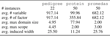
Table 1: Statistics of the three evaluated benchmark sets.

pedigree protein promedas

# instances 22 50 50

avg. # variable 917.14 99.96 682.12 avg. # of factor 917.14 355.84 682.12 avg. max domain size 4.95 77.94 2.00 avg. max scope 4.45 2.00 3.00 avg. induced width 25.50 11.24 25.76

Empirical Evaluation

In this section, we present empirical results to demonstrate the usefulness of our framework and the effectiveness of our adaptive policy.

We evaluated on three benchmarks of real-world problem instances from recent UAI competitions. Our benchmarks

include: pedigree, 22 genetic linkage instances from

the UAI’08 inference challenge1_;_protein_{, 50 instances}

made from the “small” protein side-chains of (Yanover and

Weiss 2002);promedas, 50 medical diagnosis expert

sys-tems (Wemmenhove et al. 2007). These three sets are selected to illustrate different problem characteristics. Table 1 shows some summary statistics of these benchmarks.

We adopted WMB as our variational bound, and allocated

a maximum of 512MB memory, using the largestibound

that fit our memory budget. We set a maximum time budget

of 600 seconds. The confidence parameterδfor our

proba-bilistic bounds is set to0.025. In the experiments, we also usedZδb , a (1−δ) probabilistic lower bound by the Markov

inequality (Gogate and Dechter 2011), and switched to our

lower boundZb−∆when it becomes non-trivial. We also

replacedZb+ ∆with the best deterministic upper bound

reached so far if the latter is tighter.

Table 2 explains the evaluated algorithms, all of which share the same initial WMB structure. We test our adaptive ap-proach against several non-interleaved strategies (“fixed-X”) as well as statically interleaved strategies (“static-X”). The “equal time” strategy corresponds to “static(1, tmsg/tis)”

instead of “static(tis/tmsg,1)” because message passing

is usually much more expensive than sampling (typically,

tmsg/tis>103). Note that “static (0, 1)” can also be viewed

as an optimize-first (non-interleaving) strategy “fixed 0%”, because it does not spend any time improving the variational bound after the initial bound construction. During one round of message passing, i.e., one forward-backward pass (see Liu and Ihler (2011)), we do cost-shifting and weight optimiza-tion simultaneously. All implementaoptimiza-tions are in C/C++. We ran experiments on AMD Opteron 6276 processors with a clock speed of 2.3 GHz.

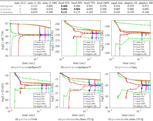
Interleaving versus Non-interleaving

Fig. 2 shows anytime bounds from some typical instances of each benchmark for interleaving and non-interleaving strate-gies. We can observe from Fig. 2 that those non-interleaving strategies except “static (0, 1)” lack good anytime behav-ior compared to our adaptive interleaving strategy: they are

1

http://graphmod.ics.uci.edu/uai08/Evaluation/Report/ Benchmarks/

Table 2: Notations and abbreviations used in figures and tables for the evaluated algorithms.

fixedp%

optimize-first policy with the firstp%of time for message passing, and the rest for sampling.

static(R, S) static policy with some given(R, S). equal time static policy with(1, tmsg/tis).

adaptiveNs adaptive policy withNspseudo samples.

unable to compute a lower bound until they quit message passing and start sampling; their early upper bounds corre-spond to the deterministic variational bounds, which typically do not improve as fast as the probabilistic upper bound of our adaptive variant. “static (0, 1)” responds quickly but often gives looser results at longer time scales; see Fig. 2(c) and 2(f) for example. It performs very well when the initial bound is already close to the ground truth (see Fig. 2(a)), but such information is usually not available to users beforehand.

To quantify the anytime performance of the methods in each benchmark, we use two measures: one is the area

be-tween the upper bound oflogZand the (estimated) ground

truth oflogZ; the other is the area between the upper and

lower bound of logZ as introduced in Lou, Dechter, and

Ihler (2017b). The first facilitates comparison with those methods that do not provide lower bounds early on. These quantities are computed for each instance and method, and then normalized by those of “static (0, 1)”. Finally, we take the (geometric) mean over these scores across each bench-mark.

From Table 3, we observe that our adaptive policy performs significantly better in terms of anytime upper bound than any of the non-interleaving variants across all the benchmarks. We can also see differences in performance stemming from the different problem characteristics in the benchmarks: for example, the performance of the non-interleaved strategies degrades with higher time used for message passing on the

pedigreebenchmark, while this is less true of the other two benchmarks; this indicates the difficulty of deciding when to quit message passing and start sampling for good anytime behavior, especially when we do not know the time limit in advance. In contrast, our interleaving framework does not have such limitations.

We also examine performance at a fixed time limit, as opposed to anytime behavior. Table 5 shows the mean final

gap between the upper bound and the (estimated)logZ. We

can see that our adaptive variants perform almost as well as the best method for each benchmark, which implies that although our algorithm is designed for a more responsive, anytime behavior, it does not sacrifice much in terms of long-term bound quality.

Adaptive versus Static

(6)

Table 3: Mean area between upper bounds and (estimated) ground truthlogZ, normalized by that of “static (0, 1)”, for each benchmark. Smaller numbers indicate better anytime upper bounds. The best for each benchmark is bolded.

static (0,1) static (1,10) static (1,100) fixed 25% fixed 50% fixed 75% fixed 100% equal time adaptive 10 adaptive 100

pedigree 1 2.436 1.262 2.084 3.027 3.904 4.655 0.947 0.781 0.786

protein 1 0.145 0.077 0.161 0.231 0.285 0.329 0.054 0.051 0.050

promedas 1 1.217 0.615 0.898 1.408 1.855 2.268 0.414 0.354 0.349

Table 4: Mean area between upper and lower bounds oflogZ, normalized by that of “static (0, 1)”, for each benchmark. Entries for some non-interleaved strategies are missing because they do not give lower bounds early on. Smaller numbers indicate better anytime bounds. The best for each benchmark is bolded.

pedigree 1 4.624 2.213 - - - - 2.061 1.544 1.529

protein 1 0.299 0.118 - - - - 0.104 0.080 0.078

promedas 1 2.674 1.203 - - - - 1.271 0.728 0.726

Table 5: Mean final gap between upper bound and (estimated) ground truthlogZ, normalized by that of “static (0, 1)”, for each benchmark. Smaller numbers are better; the best method for each benchmark is bolded.

pedigree 1 2.113 0.804 0.468 0.480 0.581 6.576 0.534 0.554 0.572

protein 1 0.045 0.016 0.004 0.004 0.005 0.208 0.005 0.006 0.005

promedas 1 0.879 0.308 0.121 0.133 0.185 2.519 0.165 0.150 0.148

102

time (sec)

-92 -91 -90 -89 -88 -87

logZ (-88.778)

static (0, 1) fixed 25% fixed 50% fixed 75% fixed 100% adaptive 100

(a)pedigree/pedigree23

100 102

time (sec) -285

-280 -275 -270 -265 -260

logZ (-268.435)

(b)pedigree/pedigree37

100 102

time (sec) -160

-140 -120 -100

logZ (-115.288)

(c)protein/1qsq

100 102

time (sec) -70

-60 -50 -40 -30

logZ (-42.043)

(d)protein/1whi

102 time (sec) -35

-30 -25 -20 -15

logZ (-19.410)

(e)promedas/or chain 132.fg

100 102

time (sec)

-40 -30 -20 -10

logZ (-20.015)

(f)promedas/or chain 153.fg

Figure 2: Anytime bounds onlogZfor two instances per benchmark, comparing our adaptive interleaving strategy with

(7)

102 time (sec) -92

-91 -90 -89 -88 -87

logZ (-88.778)

static (0, 1) static (1, 10) static (1, 100) equal time adaptive 10 adaptive 100

(a)pedigree/pedigree23

100 102

time (sec) -285

-280 -275 -270 -265 -260

logZ (-268.435)

(b)pedigree/pedigree37

100 102

time (sec) -160

-140 -120 -100

logZ (-115.288)

(c)protein/1qsq

100 102

time (sec) -70

-60 -50 -40 -30

logZ (-42.043)

(d)protein/1whi

102 time (sec) -35

-30 -25 -20 -15

logZ (-19.410)

(e)promedas/or chain 132.fg

100 102

time (sec) -40

-30 -20 -10

logZ (-20.015)

(f)promedas/or chain 153.fg

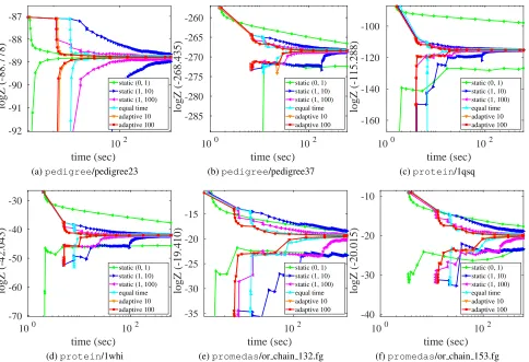
Figure 3: Anytime bounds onlogZfor two instances per benchmark, comparing our adaptive strategy with statically interleaved

strategies balancing message updates and sampling (see Table 2). The best fixed strategy is typically “equal time”, but adaptivity is usually slightly better, as it is able to change its behavior dynamically based on the observed improvement in bounds from message updates.

“equal time” variant performs better than a static choice of interleaving rate, since it is able to take into account how computationally expensive the message updates are. Even so, both of our adaptive variants (corresponding to a shorter or longer horizon when estimating the impact of a message update) perform better most of the time; they are able to make more informed decisions about the current benefits of sampling versus message updates. These observations are also supported by the statistical results in Table 3 and Table 4. From Fig. 3, Table 3, and Table 4, we can also see that the two adaptive variants perform fairly similarly. In fact, we found in our experiments that our adaptive policy works reasonably well within a wide range ofNs, i.e., it is not very sensitive to

the hyperparameter value, which simplifies its use in practice.

Conclusion

In this work, we propose a general framework that interleaves optimization of a variational upper bound with importance sampling based on its associated proposal, to obtain high-quality anytime bounds and estimates of the partition func-tion. This framework can be viewed as a meta-algorithm for

convex variational bounds such as TRW and WMB, giving them more responsive bounds without sacrificing long-term quality. Our proposed adaptive policy, which selects the ac-tion with larger unit gain for improving the probabilistic upper bound at each iteration, leads to excellent empirical anytime performance, both in comparison to simple non-interleaved baselines as well as simpler non-interleaved policies within our framework. Our approach is easy to use in practice since it does not appear to be sensitive to its hyperparame-ter in our experiments. For future work, one may consider incorporating importance sampling in the initial bound con-struction as well, to further boost the anytime performance.

Acknowledgements

We thank all the reviewers for their helpful feedback.

(8)

References

Broka, F.; Dechter, R.; Ihler, A.; and Kask, K. 2018.

Ab-straction sampling in graphical models. InProceedings of

the 34th Conference on Uncertainty in Artificial Intelligence, UAI’18.

Chakraborty, S.; Fremont, D. J.; Meel, K. S.; Seshia, S. A.; and Vardi, M. Y. 2014. Distribution-aware sampling and

weighted model counting for SAT. InProceedings of the

28th AAAI Conference on Artificial Intelligence, AAAI’14, 1722–1730.

Chakraborty, S.; Meel, K. S.; and Vardi, M. Y. 2016. Algorith-mic improvements in approximate counting for probabilistic

inference: From linear to logarithmic SAT calls. In

Proceed-ings of the 25th International Joint Conference on Artificial Intelligence, IJCAI’16, 3569–3576.

Dagum, P., and Luby, M. 1997. An optimal approximation algorithm for Bayesian inference.Artificial Intelligence 93(1-2):1–27.

Darwiche, A. 2009.Modeling and reasoning with Bayesian

networks. Cambridge University Press.

Dechter, R., and Rish, I. 2003. Mini-buckets: A

gen-eral scheme of approximating inference. Journal of ACM

50(2):107–153.

Dechter, R.; Geffner, H.; and Halpern, J. Y. 2010.Heuristics, Probability and Causality. A Tribute to Judea Pearl. College Publications.

Dechter, R. 1999. Bucket elimination: A unifying framework for reasoning.Artificial Intelligence113(1-2):41–85. Dechter, R. 2013. Reasoning with probabilistic and determin-istic graphical models: Exact algorithms.Synthesis Lectures on Artificial Intelligence and Machine Learning7(3):1–191. Ermon, S.; Gomes, C.; Sabharwal, A.; and Selman, B. 2013. Taming the curse of dimensionality: Discrete integration by hashing and optimization. InProceedings of the 30th Interna-tional Conference on InternaInterna-tional Conference on Machine Learning, ICML’13, 334–342.

Ermon, S.; Gomes, C.; Sabharwal, A.; and Selman, B. 2014. Low-density parity constraints for hashing-based discrete

integration. InProceedings of the 31st International

Con-ference on International ConCon-ference on Machine Learning, ICML’14, 271–279.

Friedman, T., and Van den Broeck, G. 2018. Approximate knowledge compilation by online collapsed importance

sam-pling. arXiv preprint arXiv:1805.12565.

Globerson, A., and Jaakkola, T. 2007. Approximate inference

using conditional entropy decompositions. InProceedings of

the 11th International Conference on Artificial Intelligence and Statistics, AISTATS’07, 131–138.

Gogate, V., and Dechter, R. 2011. Sampling-based lower bounds for counting queries.Intelligenza Artificiale5(2):171– 188.

Henrion, M. 1991. Search-based methods to bound diagnos-tic probabilities in very large belief nets. InProceedings of the 7th conference on Uncertainty in Artificial Intelligence, UAI’91, 142–150.

Liu, Q., and Ihler, A. 2011. Bounding the partition function using H¨older’s inequality. InProceedings of the 28th Interna-tional Conference on InternaInterna-tional Conference on Machine Learning, ICML’11, 849–856.

Liu, Q.; Fisher, III, J. W.; and Ihler, A. 2015. Probabilistic

variational bounds for graphical models. InAdvances in

Neu-ral Information Processing Systems, NIPS’15, 1432–1440. Liu, J. S. 2008. Monte Carlo strategies in scientific comput-ing. Springer Science & Business Media.

Lou, Q.; Dechter, R.; and Ihler, A. 2017a. Anytime anys-pace AND/OR search for bounding the partition function. InProceedings of the 31st AAAI Conference on Artificial Intelligence, AAAI’17, 860–867.

Lou, Q.; Dechter, R.; and Ihler, A. 2017b. Dynamic im-portance sampling for anytime bounds of the partition

func-tion. InAdvances in Neural Information Processing Systems,

NIPS’17, 3198–3206.

Maurer, A., and Pontil, M. 2009. Empirical Bernstein bounds and sample variance penalization. InProceedings of the 22nd Conference on Learning Theory, COLT’09.

Popoviciu, T. 1935. Sur les ´equations alg´ebriques ayant

toutes leurs racines r´eelles. Mathematica9:129–145.

Valiant, L. 1979. The complexity of computing the

perma-nent. Theoretical Computer Science8(2):189–201.

Viricel, C.; Simoncini, D.; Barbe, S.; and Schiex, T. 2016. Guaranteed weighted counting for affinity computation:

Be-yond determinism and structure. InInternational Conference

on Principles and Practice of Constraint Programming, 733– 750. Springer.

Wainwright, M., and Jordan, M. 2008. Graphical models, exponential families, and variational inference. Foundations and TrendsR in Machine Learning1(1-2):1–305.

Wainwright, M.; Jaakkola, T.; and Willsky, A. 2005. A new

class of upper bounds on the log partition function. IEEE

Transactions on Information Theory51(7):2313–2335. Wemmenhove, B.; Mooij, J. M.; Wiegerinck, W.; Leisink, M.; Kappen, H. J.; and Neijt, J. P. 2007. Inference in the

promedas medical expert system. InConference on Artificial

Intelligence in Medicine in Europe, 456–460. Springer. Yanover, C., and Weiss, Y. 2002. Approximate inference

and protein-folding. In Advances in Neural Information