A LARGE PARAMETER SPECTRAL PERTURBATION METHOD FOR NONLINEAR SYSTEMS OF PARTIAL DIFFERENTIAL EQUATIONS THAT MODELS BOUNDARY LAYER FLOW PROBLEMS

(1)

1

Frontiers in Heat and Mass Transfer

Available at

www.ThermalFluidsCentral.org

A LARGE PARAMETER SPECTRAL PERTURBATION

METHOD FOR NONLINEAR SYSTEMS OF PARTIAL

DIFFERENTIAL EQUATIONS THAT MODELS BOUNDARY

LAYER FLOW PROBLEMS

T. M. Agbajea,b_{, S. S. Motsa}a,∗_{, S. Mondal}c,†_{, P. Sibanda}a

a_{School of Mathematics,Statistics and Computer Sciences, University of KwaZulu-Natal, Pietermaritzburg, Private Bag X01 Scottsville-3209, South}

Africa

b

DST-NRF Centre of Excellence in Mathematical and Statistical Sciences (CoE-MaSS), Private Bag 3, Wits 2050, Johannesburg, South Africa

c_{Department of Mathematics, Amity University, Kolkata, Newtown- 700135,West Bengal, India}

ABSTRACT

In this work, we present a compliment of the spectral perturbation method (SPM) for solving nonlinear partial differential equations (PDEs) with applications in fluid flow problems. The (SPM) is a series expansion based approach that uses the Chebyshev spectral collocation method to solve the governing sequence of differential equation generated by the perturbation series approximation. Previously the SPM had the limitation of being used to solve problems with small parameters only. This current investigation seeks to improve the performance of the SPM by doing the series expansion about a large parameter. The new method namely the large parameter spectral perturbation method (LSPM) combines the idea of asymptotic analysis approach with numerical solution techniques. In the (LSPM), the resulting equations from the asymptotic expansion are solved numerically using the Chebyshev spectral method. The purpose of this study is to extend the existing spectral perturbation method (SPM) which was used for small parameters to be suitable for problems with large parameters. The applicability of the (LSPM), is tested on systems of earlier reported nonlinear partial differential equations that describe boundary layer fluid flow problems. The validity of the (LSPM) numerical solutions is verified by comparing with published results and the bivariate Chebyshev spectral quasilinearisation method (BSQLM) and an excellent agreement were observed. The (BSQLM) is a numerical method that blends the quasilinearisation method, the Chebyshev spectral method, and the bivariate Lagrange interpolation method. One of the advantages of this approach is that it gives results in a fraction of seconds. We remark also that simple decoupled linear systems formulas are derived for generating the solutions in the form of decoupled linear systems. Tables are generated to present error and convergence properties of the LSPM.

Keywords:Spectral Perturbation Method; Bivariate Chebyshev spectral quasilinearisation method; Chebyshev spectral collocation method.

1. INTRODUCTION

Nonlinear partial differential equations (PDEs) arise in various fields of science and engineering problems such as mathematical modelling, heat transfer, fluid mechanics, quantum mechanics and many applications in biological process. In addition, there is a large volume of published litera-ture describing the numerous important of engineering and science appli-cations of boundary layer flows. Examples include the cooling and drying of paper and textiles, aerodynamic extrusion of plastic sheets, cooling of metallic plates in a cooling bath. The equations defined by systems of nonlinear partial differential equations (PDEs) are often difficult to solve exactly. As a result of the difficulties often encountered in solving these nonlinear partial differential equations exactly, some researchers have

de-∗

University of Swaziland, Private Bag 4, Kwaluseni, Matsapha M201, Swaziland

†

Corresponding author. Email: [email protected]

veloped both numerical and analytical method for finding analytical and approximate solutions to these complicated nonlinear partial differential equations. These numerical and analytical methods have their own advan-tages and limitations. Hence, there is need to improve the performance of these existing numerical and analytical methods.

(2)

DOI: 10.5098/hmt.9.36 ISSN: 2151-8629 the impulsive motion of a stretching surface equations and employed the

asymptotic method to obtain asymptotic solutions for large values of the independent variable. Free convection in micropolar fluids over a uni-formly heated vertical plate was investigated byGorla et al.(1998) and asymptotic solutions were presented for distances away from the lead-ing edge. Bhattacharyya(2013) examined boundary layer stagnation-point flow of Casson fluid and heat transfer towards a shrinking/stretching sheet is studied. Recently,Oyelakin et al.(2017) studied the effects of thermal radiation, heat and mass transfer on the unsteady magnetohy-drodynamic(MHD) flow of a three dimensional Casson nanofluid using the spectral quasi-linearisation method. The partial differential equations governing the unsteady MHD flow on a rotating cone in a rotating fluid were solved byRoy et al.(1998), asymptotic solutions were presented for large magnetic parameterM. Natural convection flow from a ver-tical permeable flat plate with variable surface temperature and species concentration was studied byHussain et al.(2000) using the perturba-tion method, asymptotic method, local non-similarity method and Keller-box method. Saha et al.Saha et al.(2007) used the regular perturbation method, asymptotic method, implicit finite difference method together with Keller-box scheme, and the local non-similarity method to solve the effect of Hall current on the MHD laminar natural convection flow from a vertical permeable flat plate with uniform surface temperature.Slaouti et al.(2002) solved the equations modelling the spin-up and spin-down of a viscous fluid over a heated disk rotating in a vertical plane in the presence of a magnetic field and a buoyancy force and also developed an asymptotic analysis for a large magnetic parameter. An asymptotic solution for large values of the independent variableηwas generated by Takhar et al.(2001) who investigated the unsteady MHD-boundary-layer of a source and vortex flow adjacent to a stationary surface and obtained a closed form solution for large values of the suction parameter. The above-mentioned authors solved the resulting asymptotic perturbation equations analytically and their results only yield the first, second and a maximum of a third-order asymptotic solution. The problem associated with the an-alytical approach used by all the above-mentioned authors in solving the resulting asymptotic perturbation equations is that higher order asymp-totic perturbation equations may be impossible to solve exactly beyond a maximum of third-order approximation. This is because it takes far too long to generate higher order solution even with the use of a computer.

This current investigation serves to first present a Chebyshev spec-tral based approach that addresses the problem encountered by previous researchers on this subject in attempting to solve higher order asymp-totic perturbation equations exactly. The method namely the large pa-rameter spectral perturbation method (LSPM) is a method which blends the idea from asymptotic analysis with numerical solution techniques. The Chebyshev spectral method is used to obtain a numerical approxi-mate solution of the higher order asymptotic perturbation approximations which may be impossible to solve exactly. We demonstrate that using the Chebyshev spectral method to integrate the higher order asymptotic per-turbation equations gives very accurate numerical results even for com-plicated nonlinear partial differential equations in a computationally fast manner. The Chebyshev spectral was chosen in this work because spec-tral methods are well documented for their high level of accuracy and also with the spectral methods only few grid points are required to obtain accurate results. In addition, we show that using the spectral methods leads to a significant saving in computational time. This is in contrast with the analytical approach earlier employed by previous researchers because, in the analytical approach, it takes too long to solve higher or-der asymptotic equations even with the use of a scientific software but with the spectral methods, higher order asymptotic solutions are gener-ated in a fraction of seconds. Secondly, in this present study, we aim to introduce the (LSPM) as a compliment of the existing spectral perturba-tion method (SPM) which was used for small parameters and its limited in its application. The (SPM) is limited in the sense that the (SPM) is valid for small parameters and the (LSPM) approach is valid for large

parameters. The (SPM) is a series expansion based method that extends the use of the traditional perturbation scheme coupled with the Cheby-shev spectral method. The (SPM) was used in the study carried out by Agbaje and Motsa(2015) to address some of the drawbacks of the tra-ditional perturbation method and the approach was able to correct some of the conclusions drawn by researchers regarding perturbation methods. It was observed in the study conducted byAgbaje and Motsa(2015) on the SPM that the approach though accurate is not suitable for large pa-rameters. As a result of that observation made on the (SPM), we aim to extend the range of validity of the (SPM) by expanding about a large physical parameter so as to make the usual (SPM) robust and extends its application to new areas. Also, we show that the convergence speed of the usual (SPM) can be improved even whenξis large by doing the series expansion about a large physical parameter. Furthermore, simple decou-pled linear systems formulas for generating the solutions in the form of decoupled linear systems were derived in this study. This is an advan-tage of this method because the derived simple linear systems formulas enable us to solve the equations independently of each other. In order to demonstrate the applicability of the (LSPM), we consider three earlier re-ported boundary layer flow problem modelled by coupled systems of two and three nonlinear PDEs. The accuracy of the (LSPM) numerical results was compared with the bivariate quasilinearisation method (BSQLM) and the published results ofSaha et al.(2007) andHossain and Paul(2001a,b) and a good agreement was observed.

2. GOVERNING SYSTEMS OF NONLINEAR PARTIAL DIFFERENTIAL EQUATIONS

In this section, we present the systems of nonlinear partial differential equations (PDEs) that describes the different types of boundary layer flows that will be investigated in this study. In order to demonstrate the applicability of the (LSPM) numerical method of solution, we consider three various types of nonlinear PDEs.

2.1. Effect of Hall current on the MHD laminar natural convection flow from a vertical permeable flat plate with uniform surface temperature

We consider the effect of hall current on the MHD laminar natural con-vection flow from a vertical permeable flat plate with uniform surface temperature investigated by Saha et al.Saha et al.(2007). The governing nonlinear partial differential equations are given inSaha et al.(2007) in dimensionless form as:

f000+3 4f f

00 −1

2f

02₊_ξf00₊_θ

− M

(1 +m2₎ f

0₊_mg₌ 1

4ξ

f0∂f

0

∂ξ −f

00∂f

∂ξ

,

(1)

g00+3 4f g

0 −1

2f 0

g+ξg0− M

(1 +m2₎ g−mf

0

=1 4ξ

f0∂g ∂ξ −g

0∂f

∂ξ

,

(2)

1

P rθ

00 +3

4f θ 0

+ξθ0=1 4ξ

f0∂θ

0

∂ξ −θ

0∂f

∂ξ

. (3)

In the above equation, M is the magnetic field,ξ is the transpiration parameter,mis the hall parameter,(P r =v/α)is the Prandtl number and prime denotes differentiation of the functions with respect toη. The corresponding boundary conditions to the above equations are:

f(ξ,0) =f0(ξ,0) = 0, g(ξ,0) = 0, θ(ξ,0) = 1, f0(ξ,∞) =g(ξ,∞) =θ(ξ,∞) = 0. (4)

The physical quantities of interest are the skin-friction and Nusselt num-ber, which may be calculated from the following expressions and are given inSaha et al.(2007) as:

Cf xGr

−3/4

x =f

00

(ξ,0), N uxGr

−1/4 x =−θ

0

(3)

2.2. Free convection from a vertical permeable circular cone with non-uniform surface temperature

We investigate a steady two-dimensional laminar free convection flow past a non-isothermal vertical porous cone with variable surface tempera-ture. The governing non-similarity system of partial differential equations are expressed in dimensionless form asHossain and Paul(2001a):

f000+n+ 7 4 f f

00 −n+ 1

2 f

02₊_θ₊_ξf00 = 1−n

4 ξ

f0∂f

0

∂ξ −f

00∂f

∂ξ

, (6)

1

P rθ

00 +n+ 7

4 f θ 0

−nf0θ+ξθ0= 1−n 4 ξ

f0∂θ ∂ξ −θ

0∂f

∂ξ

, (7)

whereP r=ν/αis the Prandtl number,ξis the dimensionless suction parameter. The appropriate corresponding boundary conditions are;

f(ξ,0) = 0, f0(ξ,0) = 0, f0(ξ,∞) = 0,

θ(ξ,0) = 1, θ(ξ,∞) = 0. (8)

The skin friction coefficientCf xand the Nusselt numberN uxdescribe

the shear-stress and heat flux rate at the surface, respectively, and are defined byHossain and Paul(2001a) as:

Cf xGr1x/4=f

00

(ξ,0), N ux

Grx1/4

=−θ0(ξ,0). (9)

2.3. Free convection from a vertical permeable circular cone with non-uniform surface heat flux

We consider a steady two-dimensional laminar free convection flow of a viscous incompressible fluid with temperature,T, from a vertical porous cone with variable heat flux. The governing systems of nonlinear partial differential equations are given inHossain and Paul(2001b) in dimen-sionless form as:

f000+m+ 9 5 f f

00

−2m+ 3

2 f

02₊_φ₊_ξf00 =1−m

5 ξ

f0∂f

0

∂ξ −f

00∂f

∂ξ

,

(10)

1

P rφ

00₊m+ 9 5 f φ

0

−4m+ 1 5 f

0_φ₊_ξφ0₌ 1−m 5 ξ

f0∂φ ∂ξ −φ

0∂f

∂ξ

, (11)

whereP r =ν/αis the Prandtl number. The corresponding boundary conditions areHossain and Paul(2001b);

f(ξ,0) = 0, f0(ξ,0) = 0, f0(ξ,∞) = 0,

φ0(ξ,0) =−1, φ(ξ,∞) = 0. (12) The skin friction coefficientCf xand the Nusselt numberN uxdescribe

the shear-stress and heat flux rate at the surface, respectively, and are defined byHossain and Paul(2001b) as:

1 2Cf xGr

1/5 x =f

00

(ξ,0),

N ux

Gr1x/5

= 1

φ(ξ,0). (13)

3. METHOD OF SOLUTION

In this section, we present the large parameter spectral perturbation method (LSPM) solution for the problems described in the previous section. Asymp-totic perturbation analysis is carried out on the set of partial differential equations described in the previous section and the resulting differential equations are solved using the Chebyshev spectral method. Perturbation methods, in general, construct a solution for a problem by generating series expansions of the perturbation parameter. In perturbation meth-ods, higher order perturbation approximations are difficult to get which may result in less accurate results if only one or two series solutions are used. For instance, Hossain and Paul(2001a,b) presented the first order asymptotic approximate solutions for large perturbation parame-ter using the analytical approach. Hossain and Paul(2001a,b) analytical

approach yielded only the first order approximate asymptotic solution be-cause higher order solutions may be difficult to obtain exactly even with the use of a computer. Below, the development of the large parameter per-turbation approach and the application of the Chebyshev spectral method to solve the resulting ordinary differential equations is being discussed.

3.1. Large Parameter Spectral Perturbation Method Solution for large(ξ)for Equations (1-3)

We shall give attention to the solutions of equations (1-3) whenξ is large. The order of magnitude of different terms in (1-3) shows that the largest in (1) aref000andξf00, in (2)g00andξg0, andθ00andξθ0in (3). Both the terms have to be balanced in the respective equations and the only way to do this is to assume thatηto be small and its derivatives are large. Given thatθ=O(1)asξ→ ∞, it is necessary to find appropriate scaling forf andη. On balancing thef000,θandξf00terms in (1), it is found that η = O(ξ−1₎_and_f ₌ _O₍_ξ−3₎_as_ξ _{→ ∞}_{. Therefore,}

the following transformations are introduced to switch the equations for smallξto those for largeξ;

f=ξ−3F(ξ,η¯), η¯=ξη, g=ξ−2G(ξ,η¯), θ= Θ(ξ,η¯). (14) Substituting these transformations given in (14) into equations (1-3), we obtain the following equations:

F000+F00+ Θ− M (1 +m2₎ξ

−2 _F0₊_mG₌1

4ξ

−3_F0∂F0

∂ξ −F

00∂F

∂ξ

,

(15)

G00+G0− M (1 +m2₎ξ

−2 _G

−mF0₌1

4ξ

−3_F0∂G

∂ξ −G

0∂F

∂ξ

, (16)

Θ00+P rΘ0=1 4P rξ

−3_F0∂Θ

∂ξ −Θ

0∂F

∂ξ

. (17)

The corresponding boundary conditions are given as ;

F(ξ,0) =F0(ξ,0) = 0, G(ξ,0) = 0, Θ(ξ,0) = 1,

F0(ξ,∞) =G(ξ,∞) = Θ(ξ,∞) = 0. (18) Sinceξ is large, solutions of equations (15- 17) is obtained using the perturbation method. Hence, we expand the functionsF(¯η),G(¯η)and Θ(¯η)in powers ofξ−2

as given below;

F(ξ,η¯) =

∞

X

k=0

ξ−2kFk(¯η), (19)

G(ξ,η¯) =

∞

X

k=0

ξ−2kGk(¯η), (20)

Θ(ξ,η¯) =

∞

X

k=0

ξ−2kΘk(¯η). (21)

Substituting equations (19-21) into equations (15) - (17) and then equat-ing the coefficients of like powers ofξ, we obtain the equations fork= 0 as;

F0000+F

00

0 + Θ0= 0, (22)

G000 +G

0

0= 0, (23)

Θ000+P rΘ

0

0= 0, (24)

subject to the following boundary conditions

F0(0) =F00(0) = 0, G0(0) = 0, Θ0(0) = 1,

F00(∞) =G0(∞) = Θ0(∞) = 0. (25)

The equations fork= 1, corresponding to orderO(ξ−2₎

are given as;

F1000+F

00

1 =

M

(1 +m2₎ F

0

0+mG0

−Θ1, (26)

G001 +G

0

1=

M

(1 +m2₎ G0−mF

0

, (27)

Θ001 +P rΘ

0

(4)

DOI: 10.5098/hmt.9.36 ISSN: 2151-8629 subject to the following boundary conditions

F1(0) =F

0

1(0) = 0, G1(0) = 0, Θ1(0) = 0,

F10(∞) =G1(∞) = Θ1(∞) = 0. (29)

The equations fork≥2are given as;

F_k000+F_k00+ Θk=

M

(1 +m2₎F

0 k−1+

M

(1 +m2₎mGk−1

−1 2

 

k−2

X

n=0

F_k0₋₂₋_nnF_n0 − k−2

X

n=0

F_k00₋₂₋_nnFn



, (30)

G00_k+G0_k= M

(1 +m2₎Gk−1− M

(1 +m2₎mF

0 k−1,

−1 2

 

k−2

X

n=0

F_k0₋₂₋_nnGn− k−2

X

n=0

G0_k₋₂₋_nnFn



 (31)

Θ00_k+P rΘ0_k=−1 2P r

 

k−2

X

n=0

F_k0₋₂₋_nnΘn− k−2

X

n=0

Θ0_k₋₂₋_nnFn

  (32)

Fk(0) =Fk0(0) = 0, Gk(0) = 0, Θk(0) = 0,

Fk0(∞) =Gk(∞) = Θk(∞) = 0. (33)

Solving equations (22-28) analytically yields:

F0(¯η) =

1

P r2 +

e−η¯ P r(1−P r)−

e−P rη¯

P r2₍₁₋_{P r}₎, (34)

G0(¯η) = 0, (35)

Θ0(¯η) =e

−P rη¯

, (36)

F1( ¯η) =

MheP rη¯₋_e−η¯ _{P r}_{+ (}₋_{1 +}_{P r}₎ _eη¯ ₋_{1 +}_{P r}2

−P r2_{(1 + ¯}_η₎i

(1 +m2_{) (}₋_{1 +}_{P r}₎2_{P r}3 ,

(37)

G1( ¯η) =

mMhe−P rη¯+eη¯ −1−P rη¯+P r2η¯i

(1 +m2_{) (}₋_{1 +}_{P r}₎2_{P r}2 , (38)

Θ1( ¯η) = 0. (39)

The Chebyshev spectral collocation method is then applied to integrate (30-32). It is important to note that the spectral method is based on the Chebyshev polynomials defined on the domain[−1,1]by

Tl(x) = cos

lcos−1(x)

. (40)

Before using the spectral method, it is necessary to first transform the physical domain on which the governing equation is defined to the region [−1,1]where the spectral method can then be applied. This can be done with the aid of the domain truncation procedure, the problem is solved in the interval[0, L]in place of[0,∞), whereLis the scaling parameter taken to be large. The transformationx= 2 ¯_Lη −1, −1≤x≤ 1,is used to map the domain[0, L]to[−1,1]. The Gauss-lobatto collocation pointsTrefethen(2000) are used to define the Chebyshev nodes[−1,1] as;

xj= cos

πj Nx

, −1≤x≤1, j= 0,1,2..., Nx, (41)

where (Nx+ 1) is the total number of collocation points.

The basic idea behind the spectral collocation method is the intro-duction of the chebyshev differential matrixD(see for example,Trefethen (2000),Canuto et al.(1988)). The chebyshev differential matrixDis used to approximate the derivatives of the unknown variablesFk(¯η), Gk(¯η),Θk(¯η)

at the collocation points as the matrix vector product

dFk

dη¯

¯ η= ¯ηj

=

Nx

X

l=0

DjlFk(xl) =DFk, j= 0,1, ..., Nx, (42)

dGk

dη¯

¯ η= ¯ηj

=

Nx

X

l=0

DjlGk(xl) =DGk, j= 0,1, ..., Nx, (43)

dΘk

dη¯

¯ η= ¯ηj

=

Nx

X

l=0

DjlΘk(xl) =DΘk, j= 0,1, ..., Nx, (44)

where(Nx+ 1)is the number of collocation points,D= 2D/L, and

Fk= [Fk(x0), Fk(x1), ..., Fk(xNx)]

T

, (45)

Gk= [Gk(x0), Gk(x1), ..., Gk(xNx)]

T

, (46)

Θk= [Θk(x0),Θk(x1), ...,Θk(xNx)]

T

, (47)

is the vector function at the collocation points. We obtain the higher order derivatives as powers ofD, that is;

F(_kp)=DpFk, G(kp)=D p

Gk, Θ(kp)=D p

Θk, (48)

wherepis the order of the derivatives. The matrixD is of size (Nx+ 1)×(Nx + 1)and its entries are defined inTrefethen(2000);

Canuto et al.(1988) as;

Djl=

cj

cl

(−1)j+l

τj−τl

j6=l;j, l= 0,1,2, N,

Dll=−

τl

2(1−τ2 l)

1≤j=l≤N−1,

D00=

2N2+ 1

6 = −DNxNx, (49)

with

cl=

(

2, l= 0, Nx

−1, −1≤l≤Nx−1.

(50)

Substituting (42-48) in (30-32) yields

A1,k−1Fk=B1,k−1, A2,k−1Gk=B2,k−1, A3,k−1Θk=B3,k−1, (51)

Nx

X

l=0

D0lFk(xl) = 0, Nx

X

l=0

DNxlFk(xl) = 0, Fk(xNx) = 0, (52)

Gk(xNx) = 0, Gk(x0) = 0, (53)

Θk(xNx) = 0, Θk(x0) = 0, (54)

whereA1,k−1,A2,k−1,A3,k−1,B1,k−1,B2,k−1,andB3,k−1are defined

as;

A1,k−1=D3+D2, A2,k−1=D2+D, A3,k−1=D2+D, (55)

B1,k−1=

M

(1 +m2₎(DFk−1) +

M

(1 +m2₎mGk−1−Θk+SumF,

(56)

B2,k−1=

M

(1 +m2₎Gk−1−

M

(1 +m2₎m(DFk−1) +SumG, (57)

B3,k−1=SumΘ, (58)

where SumF,SumGand SumΘare defined as;

SumF=−1

2

k−2

X

n=0

(DFk−2−n) (nDFn)− D2Fk−2−n

(nFn)

,

SumG=−1

2

k−2

X

i=0

[(DFk−2−n) (nGn)−(DGk−2−n) (nFn)],

SumΘ=−1

2P r

k−2

X

i=0

(5)

The boundary condition (52) is imposed on the first ,Nxthrow

(second from the last row) and(Nx+ 1)st row (last row) rows and first

and last columns ofA1,k−1Fk=B1,k−1to obtain        

D0,0 D0,1 · · · D0,Nx−1 D0,Nx

A1,k−1

D_Nx,0 D_Nx,1 · · · D_Nx,Nx−1 D_Nx,Nx

0 0 · · · 0 1

                

Fk(x0 )

Fk(x1 )

. . . Fk(_xNx−1 )

Fk(_xNx)

         =            0

B₁_,k₋_{1 (}x_{1 )} . . . B₁_,k−1 (xNx−1 )

0 0            (59)

while the boundary conditions (53) and (54) are imposed the first and last rows and columns ofA2,k−1Gk=B2,k−1andA3,k−1Θk=B3,k−1

respectively, to obtain:

    

1 0 · · · 0 0

A2,k−1

0 0 · · · 0 1

         

Gk(x0) Gk(x1)

. . .

Gk(xNx)

     =        0

B2,k−1(x1)

. . .

B2,k−1(xNx−1)

0        , (60) and     

1 0 · · · 0 0

A3,k−1

0 0 · · · 0 1

         

Θk(x0)

Θk(x1)

. . .

Θk(xNx)

     =        0

B3,k−1(x1)

. . .

B3,k−1(xNx−1)

0        . (61)

Therefore, starting from a knownF0,Θ0,Φ0, the solutionsFk, Gk,Θk,

fork≥2can be obtained from equations (59-61) as;

Fk=A

−1

1,k−1B1,k−1, Gk=A

−1

2,k−1B2,k−1, Θk=A

−1

3,k−1B3,k−1.

(62)

3.2. Large parameter Spectral Perturbation Method Solution for large(ξ)for Equations (6-7)

To solve equations (6- 7), attention shall be given to the solutions of equations (6and7) whenξis large. An order of magnitude of different terms in equations (6and7) shows that the largest terms in (6) aref000

andξf00, andθ00andξθ0 in (7). Both terms have to be balanced in the respective equations and the only way to do this is to assume thatηto be small and its derivatives are large. Given thatθ=O(1)asξ→ ∞, it is necessary to find appropriate scaling forfandη. On balancing thef000

,θandξf00terms in (6), it is found thatη=O(ξ−1)andf =O(ξ−3) asξ → ∞. Therefore, the following transformations are introduced to switch the equations for smallξto those for largeξ;

f=ξ−3F(ξ,η¯), η¯=ξη, θ= Θ(ξ,η¯). (63) Substituting these transformations given in (63) into equations (6-7), we obtain the following equations:

F000+F00+ Θ + (1 +n)ξ−4F F00−nξ−4F02=1−n 4 ξ

−3_F0∂F0

∂ξ −F

00∂F

∂ξ

,

(64)

Θ00+P rΘ0+ (1 +n)P rξ−4FΘ0−nP rξ−4F0Θ =1−n 4 P rξ

−3_F0∂Θ

∂ξ −Θ 0∂F ∂ξ . (65)

The corresponding boundary conditions are given by ;

F(ξ,0) =F0(ξ,0) = 0, Θ(ξ,0) = 1, F0(ξ,∞) = Θ(ξ,∞) = 0. (66)

Sinceξis large, solutions of equations (64-65) is obtained using the spectral perturbation method. Hence, we expand the functionsF(ξ,η¯), andΘ(ξ,η¯)in powers ofξ−4as given below;

F(ξ,η¯) =

∞

X

k=0

ξ−4kFk(¯η), Θ(ξ,η¯) =

∞

X

k=0

ξ−4kΘk(¯η). (67)

Substituting equation (67) into equations (64) and (65) and then equating the coefficients of like powers ofξ, we obtain the equations fork= 0as;

F0000+F

00

0 + Θ0= 0, Θ000+P rΘ

0

0= 0, (68)

F0(0) =F00(0) = 0, Θ0(0) = 1, F00(∞) = Θ0(∞) = 0. (69)

Fk000+F

00

k + Θk=n k−1

X

i=0

Fk0−1−iF

0

i−(1 +n) k−1

X

i=0

Fk−1−iF

00

i,

+ (1−n)

"_k−1

X

i=0

Fk00−1−iiFi− k−1

X

i=0

Fk0−1−iiF

0

i

#

, (70)

Θ00k+P rΘ

0

k=nP r k−1

X

i=0

Fk0−1−iΘi−(1 +n)P r k−1

X

i=0

Fk−1−iΘ

0

i,

+ (1−n)P r "k−1

X

i=0

Θ0k−1−iiFi− k−1

X

i=0

Fk0−1−iiΘi

#

(71)

Fk(0) =F

0

k(0) = 0, Θk(0) = 0, F

0

k(∞) = Θk(∞) = 0. (72)

Since the left hand side of of the higher order perturbation equations (71) - (72) are linear, we therefore apply the Chebyshev spectral collocation method described in the previous section to integrate equations (71-72). We remark that the equations atk= 0andk= 1, can be solved analyti-cally. The equations corresponding tok= 1is;

F1000+F

00

1 + (1 +n)F0F

00

0 −nF

02

0 =−Θ1,

Θ001+P rΘ

0

1+ (1 +n)P rF0Θ

0

0−nP rF

0

0Θ0= 0, (73)

subject to the following boundary conditions:

F1(0) =F10(0) = 0, Θ1(0) = 0, F10(∞) = Θ1(∞) = 0.

On solving equations (68) and (73) analytically, their solutions were ob-tained as;

F0(¯η) =

1

P r2 +

1

P r(1−P r)e

−¯η

− 1

P r2₍₁₋_{P r}₎e

−P rη¯

, (74)

Θ0(¯η) =e−P rη¯. (75)

F1( ¯η) =

(1 +P r)−2P r3_{+ 2}_{P r}2₍₁₋_{P r}₎_n

2P r4₍₁₋_{P r}2₎ −

3(1 +n)

P r4₍₁₋_{P r}₎+

1 +P r+P r2

8P r4₍₁₋_{P r}₎2,

+ P r−(1−P r)n (1−P r2₎₍₁₋_{P r}₎2+

(1 +n)(1 +P r2₎₋₂_{P rn} P r3₍₁₋_{P r}2₎2 ,

+

"

(1 +P r)−2P r3_{+ 2}_{P r}2₍₁₋_{P r}₎_n

2P r3₍₁₋_{P r}₎2_{(1 +}_{P r}₎ −

3(1 +n)

P r3₍₁₋_{P r}₎

#

e−η¯,

+

_{1 +}_{P r}

8P r3₍₁₋_{P r}₎2₍₁₋₂_{P r}₎−

P r−(1−P r)n P r(1−P r2_{)(1 +}_{P r}₎

e−η¯,

+

"

(1 +n)(1 +P r2)−2P rn P r4₍₁₋_{P r}2₎2_{(1 +}_{P r}₎ −

1 2P r2₍₁₋_{P r}₎2

#

e−η¯,

+

"

−(1 +P r)−2P r

3_{+ 2}_{P r}2₍₁₋_{P r}₎_n

2P r4(1−P r)2(1 +P r) −

3(1 +n)

P r4(1−P r)

#

e−P rη¯,

+

_{1 +}_n

P r3₍₁₋_{P r}₎η¯

e−P rη¯−

_{1 +}_n

P r3₍₁₋_{P r}₎

¯

ηe−η¯,

+

"

P r−(1−P r)n P r(1−P r2)(1 +P r)2−

(1 +n)(1 +P r2)−2P rn P r4(1−P r2)2

#

e−(1+P r) ¯η,

−

_{1 +}_{P r}

8P r4₍₁₋_{P r}₎2₍₁₋₂_{P r}₎

e−2P rη¯+ e −2 ¯η

4P r2₍₁₋_{P r}₎2. (76)

Θ1( ¯η) =

"

(1 +P r)−2P r3+ 2P r2(1−P r)n

2P r2₍₁₋_{P r}2₎ −

¯

η+nη¯

P r

#

e−P rη¯

+

_{P r}₋₍₁₋_{P r}₎_n

1−P r2

e−(1−P r) ¯η− e −2P rη¯

(6)

DOI: 10.5098/hmt.9.36 ISSN: 2151-8629 The differential matrixDis used to approximate the derivatives of

the unknown variablesFk(¯η),Θk(¯ηat the collocation points and are

de-fined as;

dFk

dη¯

¯ η= ¯ηj

=

Nx

X

l=0

DjlFk(xl) =DFk, j= 0,1, ..., Nx, (78)

dΘk

dη¯

¯ η= ¯ηj

=

Nx

X

l=0

DjlΘk(xl) =DΘk, j= 0,1, ..., Nx, (79)

whereNx+ 1is the total number of collocation points,D= 2D/L, and

Fk= [Fk(x0), Fk(x1), ..., Fk(xN x)]T,

Θk= [Θk(x0),Θk(x1),· · ·,Θk(xN x)]T, (80)

are the vector functions at the collocation points. The matrixDis of size (Nx+ 1)×(Nx+ 1)and its entries are defined in the previous section.

Substituting (78-80) in (70-71) gives

A1,k−1Fk=B1,k−1, A2,k−1Θk=B2,k−1, (81)

subject to the boundary conditions

Nx

X

l=0

D0kFk(¯ηk) = 0, Nx

X

l=0

DN xkFk(¯ηk) = 0, Fk(¯ηN x) = 0, (82)

Θk(ηN x) = 0, Θk(η0) = 0. (83)

The coefficientsA1,k−1,A2,k−1,B1,k−1,B2,k−1,are defined as;

A1,k−1=D3+D2+Θk, A2,k−1 =D2+P rD, (84)

B1,k−1=n k−1

X

i=0

(DFk−1−i) (DFi)−(1 +n) k−1

X

i=0

Fk−1−i D2Fi

+ (1−n)

"k−1

X

i=0

D2Fk−1−i(iFi)− k−1

X

i=0

(DFk−1−i) (iDFi)

#

, (85)

B2,k−1 =nP r k−1

X

i=0

(DFk−1−i) (Fi)−(1 +n)P r k−1

X

i=0

Fk−1−i(DΘi)

+ (1−n)P r "_k−1

X

i=0

(DΘk−1−i) (iFi)− k−1

X

i=0

(DFk−1−i) (iΘi)

#

.

(86)

The boundary condition (82) is imposed on the first ,Nxthrow (second

from the last row) and(Nx+ 1)st row (last row) rows and first and last

columns ofA1,k−1Fk =B1,k−1,while the boundary conditions (83) is

imposed on the first and last rows and columns ofA2,k−1Θk=B2,k−1,

. Thus, starting from a knownF0, andΘ0, the solutionsFk,andΘk, for

k≥1can be obtained as;

Fk=A

−1

1,k−1B1,k−1, Θk=A

−1

2,k−1B2,k−1. (87)

3.3. Large Parameter Spectral Perturbation Method Solution for large(ξ)for Equations (10-11)

To find the solutions of equations (10-11) along with boundary condi-tions12, attention shall be given to the solutions of equations (10-11) whenξis large. An order of magnitude of various terms carried out in equations (10-11) depicts that the largest in (10) aref000andξf00, and

φ00 andξφ0 in (11). Both terms have to be balanced in the respective equations and the only way to do this is to assume thatηis small and its derivatives are large. Given thatφ = O(ξ−1₎

asξ → ∞, it is es-sential to find appropriate scaling forfandη. On balancing thef000,φ

andξf00terms in (10), it is found thatη = O(ξ−1₎_and_f ₌ _O₍_ξ−4₎

asξ → ∞. Therefore, the following transformations are introduced to switch the equations for smallξto those for largeξ;

f=ξ−4F(ξ,η¯), η¯=ξη, φ=ξ−1Φ(η,η¯). (88) Substituting these transformations given in (88) into equations (10-11), we obtain the following equations:

F000+F00+ Φ + (1 +m)ξ−5F F00−mξ−5F02,

= 1−m 5 ξ

−4

F0∂F

0

∂ξ −F

00∂F

∂ξ

, (89)

Φ00+P rΦ0+ (1 +m)P rξ−5FΦ0−mP rξ−5F0Φ,

= 1−m 5 P rξ

−4

F0∂Φ

∂ξ −Φ

0∂F

∂ξ

. (90)

The corresponding boundary conditions are given as;

F(ξ,0) =F0(ξ,0) = 0, Φ0(ξ,0) =−1, F0(ξ,∞) = Φ(ξ,∞) = 0.

(91) The functionsF(ξ,η¯), andΦ(ξ,η¯)are expanded in powers ofξ−5 and written below as;

F(ξ,η¯) =

∞

X

k=0

ξ−5kFk(¯η), (92)

Φ(ξ,η¯) =

∞

X

k=0

ξ−5kΦk(¯η). (93)

Substituting equations (92) - (93) into equations (89) - (90) and then bal-ancing terms of same orders of ξ, we obtain the equations fork = 0 as;

F0000+F

00

0 =−Φ0, Φ000 +P rΦ

0

0= 0, (94)

F0(0) =F

0

0(0) = 0, Φ

0

0(0) =−1, F

0

0(∞) = Φ0(∞) = 0.

Fk000+F

00

k + Φk=m k−1

X

i=0

Fk0−1−iF

0

i−(1 +m) k−1

X

i=0

Fk−1−iFi00,

+ (1−m)

"k−1

X

i=0

Fk00−1−iiFi− k−1

X

i=0

Fk0−1−iiF

0

i

#

,

(95)

Φ00k+P rΦ

0

k=mP r k−1

X

i=0

Fk0−1−iΦi−(1 +m)P r k−1

X

i=0

Fk−1−iΦ0i,

+ (1−m)P r "_k−1

X

i=0

Φ0k−1−iiFi− k−1

X

i=0

Fk0−1−iiΦi

#

, (96)

Fk(0) =F

0

k(0) = 0, Φ

0

k(0) = 0, F

0

k(∞) = Φk(∞) = 0.

The equations corresponding tok= 1is;

F1000+F

00

1 + (1 +m)F0F

00

0 −mF

02 0 =−Φ1,

Φ001+P rΦ

0

1+ (1 +m)P rF0Φ

0

0−nP rF

0

0Φ0= 0, (97)

subject to the boundary conditions;

F1(0) =F10(0) = 0, Φ

0

1(0) = 0, F

0

(7)

We remark the analytical solutions obtained on solving equations (94) and (97) are:

F0( ¯η) =

1

P r3+ e−η¯ P r2₍₁₋_{P r}₎−

e−P rη¯

P r3₍₁₋_{P r}₎, (98)

Φ0( ¯η) = e−P rη¯

P r , (99)

F1( ¯η) =

1−(1 +m)(4−P r)

P r6 +

P r−m(1−P r)

P r2₍₁₋_{P r}₎2₍₁₋_{P r}2₎,

−(1 +m)(1 +P r

2₎₋₂_{mP r}

P r5₍₁₋_{P r}2₎2 +

1 +P r+ 2P r2

8P r6₍₁₋_{P r}₎2,

+

₁₋_{(1 +}_m₎₍₄₋_{P r}₎

P r5₍₁₋_{P r}₎

e−η¯−

_{P r}₋_m₍₁₋_{P r}₎

P r3_{(1 +}_{P r}₎₍₁₋_{P r}2₎

e−η¯,

+

"

1

2P r4₍₁₋_{P r}₎2−

(1 +m)(1 +P r2₎₋₂_{mP r} P r6₍₁₋_{P r}₎2_{(1 +}_{P r}₎

#

e−η¯,

+

_{1 +}_{P r}

4P r5₍₁₋_{P r}₎2₍₁₋₂_{P r}₎

e−η¯+

₋_η_¯_{+ (1 +}_m₎₍₋_{2 ¯}_η₋_{P r}_η_¯₋₁₎

P r6₍₁₋_{P r}_{) ¯}_η

e−P rη¯,

+

_{P r}₋_m₍₁₋_{P r}₎

P r3_{(1 +}_{P r}₎2₍₁₋_{P r}2₎

e−(1+P r) ¯η,

−

"

(1 +m)(1 +P r2)−2mP r P r6₍₁₋_{P r}2₎2

#

e−(1+P r) ¯η−

_{1 +}_m

P r5₍₁₋_{P r}₎η¯

e−η¯,

−

_{1 +}_{P r}

8P r6_{(1 +}_{P r}₎2₍₁₋₂_{P r}₎

e−2P rη¯+ e −2 ¯η

4P r4₍₁₋_{P r}₎2. (100)

Φ1( ¯η) =

₁₋_{(1 +}_m_{) (1}₋_{P r}₊_{P r}_η_¯₎

P r4

e−P rη¯,

+

_{P r}₋_m₍₁₋_{P r}₎

P r2(1−P r2)

e−(1+P r) ¯η− e −2P rη¯

2P r4(1−P r).

(101)

Applying the Chebyshev spectral method on equations (95) and (96) gives:

A1,k−1Fk=B1,k−1, A2,k−1Φk=B2,k−1, (102)

subject to the boundary conditions

Nx

X

l=0

D0kFk(¯ηk) = 0, Nx

X

l=0

DN xkFk(¯ηk) = 0, Fk(¯ηN x) = 0,

Φk(ηN x) = 0, Φk(η0) = 0. (103)

The coefficientsA1,k−1,A2,k−1,B1,k−1,B2,k−1,are defined as;

A1,k−1=D3+D2 A2,k−1=D2+P rD, (104)

B1,k−1=m k−1

X

i=0

(DFk−1−i) (DFi)−(1 +m) k−1

X

i=0

Fk−1−i D2Fi

+ (1−m)

"k−1

X

i=0

D2Fk−1−i

(iFi)− k−1

X

i=0

(DFk−1−i) (iDFi)

#

−Φk,

(105)

B2,k−1=mP r k−1

X

i=0

(DFk−1−n) (Φn)−(1 +m)P r k−1

X

i=0

Fk−1−i(DΦi)

+ (1−m)P r "_k−1

X

i=0

(DΦk−1−i) (iFi)− k−1

X

i=0

(DFk−1−i) (iΘi)

#

.

(106)

Thus, starting from a knownF0, andΦ0, the solutionsFk, andΦk, for

k≥1can be obtained.

4. RESULTS AND DISCUSSION

In this section, the nonlinear systems of partial differential equations (1 -3), (6-7), and (10-11) were solve numerically using the large parame-ter spectral perturbation method (LSPM). Results were presented for the

skin friction coefficient and Nusselt number for different physical param-eters that are of interest to the flow model. The accuracy of the com-puted (LSPM) approximate numerical results were confirmed by compar-ing with other reported results from literature. The comparison was done in particular against the reported results ofSaha et al.(2007) who solved equations (1-2) using regular perturbation method, asymptotic method so-lution, implicit finite difference method together with Keller-box scheme and local nonsimilarity method. In addition, comparison were also made against published results ofHossain and Paul(2001a,b) who used the fi-nite difference method, series solution method and an asymptotic solution method to respectively, solve equations (6-7) and (10-11). Validation of the numerical solutions was further established by comparing the (LSPM) results with numerical approximate solutions obtained using the bivariate quasilinearisation method (BSQLM) as described byMotsa et al.(2014) andMotsa and Ansari(2015). We remark that the values of all physical parameters used in this study were chosen based on the values used in the published work ofHossain and Paul (2001a,b);Saha et al.(2007). The number of collocation pointsNxused was60if not stated. In order

to further check the accuracy of the LSPM, we obtain the error norm of the approximate solution and the residual error. The error norm of the approximate solution can be defined as the difference between the ap-proximate values ofF,Θ, andΦat the next approximation level, which is given as;

EF =||Fm+1−Fm||∞,

EΘ=||Θm+1−Θm||∞,

EΦ=||Φm+1−Φm||∞, (107)

whereFm+1,Θm+1andΦm+1are the previous approximation level and

Fm,Θm, andΦmare the current approximation level. Furthermore, to

define the residual error, we assume thatx∗is an approximation to the solutionAx=b, the residualr=b−Ax∗. The residual error afterm

approximation over allr= 0,1,2,· · ·, Nxcan be defined as;

Res(F) = max0≤j≤Nx|N¯F[Fm(ξ, η),Θm(ξ, η)]|,

Res(Θ) = max0≤j≤Nx|N¯Θ[Fm(ξ, η),(ξ, η),Θm(ξ, η)]|,

Res(Φ) = max0≤j≤Nx|N¯Θ[Fm(ξ, η),Θm(ξ, η)]|, (108)

whereN¯F,N¯GandN¯Θare the governing nonlinear PDEs andFm(ξ, η),

Θm(ξ, η)andΦm(ξ, η)are the LSPM approximate solutions.

Table 1displays the approximate numerical solutions of the lo-cal skin-friction coefficient,Cf xGr

−3/4

x and the local Nusselt number,

N uxGr−x1/4at different values of the transpiration parameterξfor Prandtl

numberP r = 0.7, Hall parameterm = 100and magnetic parameter

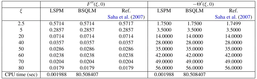
M = 0.5. The table further shows a comparison of the (LSPM), and the published work ofSaha et al.(2007). From the table, it can be seen that the (LSPM) results match perfectly well with those ofSaha et al.(2007) up to four decimal digits. In addition, it can be observed from the table that the skin-friction coefficient decreases with an increase in the values of the transpiration parameter while the local Nusselt number increases with an increase in the values of the transpiration parameter. Computed numerical values of the local skin-friction coefficient,Cf xGr

1/4 x and the

local Nusselt number,N uxGr 1/4

x for different values of the suction

pa-rameterξ, when the Prandtl numberP r= 0.10and temperature gradient

n= 0.5is displayed in Table2. It can be seen from the Table that there is an excellent agreement between our numerical results and the published result of Hossain et al. Hossain and Paul(2001a). Also, from Table2, we observe that the values of the local skin-friction coefficient decreases with an increase in the values of the suction parameter while it is noticed that an increase in the values of the suction parameter causes an increase in the values of the local Nusselt number.

Tables3depicts a comparison between our numerical values of the local skin-frictionCf xGr1x/5/2and the local Nusselt number,N uxGrx1/5

(8)

DOI: 10.5098/hmt.9.36 ISSN: 2151-8629

Table 1Comparison of LSPM and BSQLM approximate solutions forF00(0, ξ), and−Θ0(0, ξ), against those of Ref. Saha et al.(2007) at different values ofξfor Equations (1-3) whenm= 100,P r= 0.7, andM = 0.5

F00(ξ,0) −Θ0(ξ,0)

ξ LSPM BSQLM Ref. LSPM BSQLM Ref.

Saha et al.(2007) Saha et al.(2007)

2.5 0.5714 0.5714 0.5717 1.7500 1.7500 1.7499

5 0.2857 0.2857 0.2857 3.5000 3.5000 3.5000

20 0.0714 0.0714 0.0714 14.0000 14.0000 14.0000

40 0.0357 0.0357 0.0357 28.0000 28.0000 28.0000

50 0.0286 0.0286 0.0286 35.0000 35.0000 35.0000

60 0.0238 0.0238 0.0238 42.0000 42.0000 42.0000

70 0.0204 0.0204 0.0204 49.0000 49.0000 49.0000

80 0.0179 0.0179 0.0179 56.0000 56.0000 56.0000

CPU time (sec) 0.001988 80.508407 0.001988 80.508407

Table 2Comparison of LSPM and BSQLM numerical values of skin friction (F00(ξ,0)) and Nusselt number (−Θ0(ξ,0)) solutions against those of Ref.Hossain and Paul(2001a) at different values ofξfor Equations (6-7) whenn= 0.5, andP r= 0.10

F00(ξ,0) −Θ0(ξ,0)

Hossain and Paul(2001a) Hossain and Paul(2001a)

15 0.66387 0.66385 0.66378 1.50269 1.50268 1.49941

20 0.49933 0.49932 0.49932 2.00114 2.00113 1.99975

25 0.39978 0.39978 0.39978 2.50058 2.50058 2.49987

30 0.33324 0.33324 0.33324 3.00034 3.00034 2.99993

CPU time (sec) 0.006431 79.238710 0. 0.006431 79.238710

Table 3Comparison of LSPM and BSQLM numerical values of skin friction (F00(ξ,0)) and Nusselt number

ξ

Φ(ξ,0)

solutions against those of

Ref.Hossain and Paul(2001b) at different values ofξfor Equations (10-11) whenm= 0.5, andP r= 0.10

F00(ξ,0)

ξ

Φ(ξ,0)

Hossain and Paul(2001b) Hossain and Paul(2001b)

10 0.97055 0.97073 0.98963 1.00884 0.004 1.00950

20 0.24981 0.24976 0.24953 2.00057 2.00057 2.00059

30 0.11110 0.11108 0.11108 3.00011 3.00011 3.00012

40 0.06250 0.06250 0.06250 4.00004 4.00004 4.00004

50 0.04000 0.04000 0.04000 5.00002 5.00002 5.00002

CPU time (sec) 0.005100 76.914510 0.005100 76.914510

of the suction parameterξ, when Prandtl numberP r = 0.10and the heat flux gradientm = 0.5. On comparison, we observe that there is a good agreement between the (LSPM), and the approximate numerical solutions obtained byHossain and Paul(2001b). We observe from the Ta-ble4that for increased values ofξ, there is a decrease in the values of the local skin-friction, while it is noticed that asξincreases, the local Nusselt number increases. We remark that the (LSPM) is computationally faster than the (BSQLM) in terms of computational time as accurate solutions are obtained in a fraction of seconds in all the examples considered in this investigation.

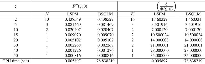
Tables4,5and8illustrates the results for the skin-friction and the Nusselt number respectively. The tables give a comparison between the (LSPM) and the (BSQLM) numerical approximate solutions and the two results are in good agreement for all values ofξconsidered. Again it can be seen from the tables that the (LSPM) gives results in a fraction of a sec-ond when compared with the (BSQLM). This is because, in the (LSPM), discretization is done only in theξ−direction while discretization is done both in theη−andξ−direction in the (BSQLM). In particular, it can be observed from the tables that only a few terms of the (LSPM) approxima-tion are required to give results presented in the tables for all large values

of ξ considered. This is a clear indication that the (LSPM) is a good numerical tool for solving nonlinear PDEs involving large parameter.

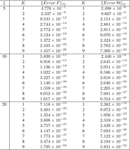
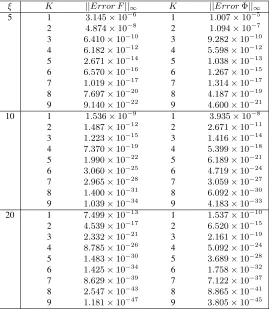
Tables7-9shows the (LSPM) maximum errors between the current and previous iteration level. The errors norm were used to measure the convergence of the solution algorithm over a number of iterations. It can be seen from the tables that even asξbecomes very large, the accuracy of the method improves. We also note from the tables that the solution error decreases with an increase in the order of LSPM approximationK. The solution error improves asξbecomes larger. This is evident from the convergence level in table7with ErrorF,EFwhich is10−16forξ= 5,

10−23_for_ξ_{= 10}_and₁₀−30_for_ξ _{= 20, ErrorΘ,}_E

Θup to10−15for

ξ = 5,10−21forξ = 10and10−27forξ = 20. In table8, accurate results with ErrorF, EF of order up to 10−26 forξ = 5, 10−42 for

ξ= 10and10−58

forξ= 20, ErrorΘ,EΘup to10−26forξ= 5,10−23

forξ = 10 and10−30 forξ = 20. Also, in table9, accurate results with ErrorF, EF of order up to10−22forξ = 5,10−34forξ = 10

and10−47

forξ = 20, ErrorΦ,EΦup to10−21forξ = 5,10−33for

(9)

Table 4Comparison between the LSPM and BSQLM numerical values of the skin frictionF00(0, ξ)and the Nusselt numberΘ0(0, ξ)at different values ofξfor Equations (1-3) whenm= 100,M= 0.5, andP r= 0.7

ξ F00(ξ,0) −Θ0(ξ,0)

K LSPM BSQLM K LSPM BSQLM

2 10 0.714266 0.714691 8 1.400001 1.400096

5 3 0.285713 0.285713 2 3.500000 3.500000

10 2 0.142857 0.142857 2 7.000000 7.000000

15 1 0.095238 0.095238 1 10.500000 10.500000

20 1 0.071429 0.071429 1 14.000000 14.000000

30 1 0.047619 0.047619 1 21.000000 21.000000

40 1 0.035714 0.035714 1 28.000000 28.000000

50 1 0.028571 0.028571 1 35.000000 35.000000

CPU time (sec) 0.009417 80.238359 0.009417 80.238359

Table 5Comparison between the LSPM and BSQLM numerical values of the skin frictionF00(0, ξ)and the Nusselt numberΘ0(0, ξ)at different values ofξfor Equations (6-7) whenn= 0.5, andP r= 0.7

ξ F00(ξ,0) −Θ0(ξ,0)

2 16 0.618112 0.618530 15 1.481166 1.481091

5 3 0.284272 0.284256 3 3.506668 3.506668

10 3 0.142812 0.142812 3 7.000840 7.000840

15 2 0.095232 0.095232 2 10.500249 10.500249

20 2 0.071427 0.071427 2 14.000105 14.000105

30 1 0.047619 0.047619 2 21.000031 21.000031

40 1 0.035714 0.035714 2 28.000013 28.000013

50 1 0.028571 0.028571 2 35.000007 35.000007

CPU time (sec) 0.009417 80.238359 0.009417 80.238359

Table 6Comparison between the LSPM and BSQLM numerical values of the skin frictionF00(0, ξ)and the Nusselt number

ξ

Φ(ξ,0)

at different

values ofξfor Equations (10-11) whenm= 0.5, andP r= 0.7

ξ F00(ξ,0)

ξ

Φ(ξ,0)

2 13 0.438549 0.438527 15 1.460329 1.460331

5 3 0.081469 0.081469 3 3.501916 3.501916

10 2 0.020407 0.020407 2 7.000120 7.000120

15 1 0.009070 0.009070 2 10.500024 10.500024

20 1 0.005102 0.005102 2 14.000008 14.000008

30 1 0.002268 0.002268 2 21.000001 21.000001

40 1 0.001276 0.001276 1 28.000000 28.000000

50 1 0.000816 0.000816 1 35.000000 35.000000

(10)

DOI: 10.5098/hmt.9.36 ISSN: 2151-8629

Table 7LSPM Convergence of solution maximum error for Equations (1-3) at different values ofξwhenm= 100,P r= 0.7,M = 0.5,L= 30, andNx= 60

ξ K ||Error F||∞ K ||ErrorΘ||∞

5 1 4.503×10−9

1 1.052×10−8

2 3.065×10−10 2 1.218×10−9 3 3.552×10−11 ₃ ₁_.₂₇₉_×₁₀−10

4 3.498×10−12 4 1.478×10−11 5 5.436×10−13 5 2.260×10−12 6 6.645×10−14

6 2.818×10−13

7 1.241×10−14 7 5.249×10−14 8 1.767×10−15 ₈ ₇_.₄₉₃_×₁₀−15

9 3.771×10−16 9 1.599×10−15 10 1 3.518×10−11 1 2.478×10−10 2 5.985×10−13 2 1.904×10−11 3 1.734×10−14

3 4.996×10−13

4 4.270×10−16 4 1.443×10−14 5 1.659×10−17 ₅ ₅_.₅₁₇_×₁₀−16

6 1.720×10−19 6 4.719×10−17 7 2.366×10−20 7 8.009×10−19 8 8.425×10−22

8 2.859×10−20

9 4.496×10−23 9 1.525×10−21 20 1 2.749×10−13 1 2.743×10−12 2 1.169×10−15 ₂ ₂_.₉₇₄_×₁₀−13

3 8.469×10−18 3 1.951×10−15 4 5.213×10−20 4 1.409×10−17 5 5.063×10−22

5 1.347×10−19

6 3.868×10−24 6 1.050×10−21 7 4.514×10−26 ₇ ₁_.₂₂₂_×₁₀−23

8 4.017×10−28 8 1.090×10−25 9 5.359×10−30 9 1.454×10−27

Table 8LSPM Convergence of solution maximum error for Equations (6-7) at different values ofξwhenn= 0.5,P r= 0.7,L= 30, andNx= 60

ξ K ||Error F||∞ K ||ErrorΘ||∞

5 1 4.776×10−7 1 2.498×10−6 2 2.337×10−9 ₂ ₈_.₆₆₇_×₁₀−9

3 9.531×10−12 3 2.151×10−11 4 2.744×10−14 4 2.881×10−14 5 2.772×10−17

5 2.811×10−16

6 3.134×10−19 6 9.070×10−19 7 1.372×10−21 ₇ ₂_.₄₂₄_×₁₀−21

8 2.435×10−24 8 2.703×10−23 9 1.457×10−26 9 7.380×10−26 10 1 5.830×10−11 1 2.440×10−9

2 8.916×10−15

2 2.645×10−13

3 1.136×10−18 3 2.051×10−17 4 1.022×10−22 ₄ ₈_.₅₈₆_×₁₀−22

5 3.227×10−27 5 2.618×10−25 6 1.140×10−30 6 2.640×10−29 7 1.559×10−34

7 2.205×10−33

8 8.652×10−39 8 7.681×10−37 9 1.617×10−42 ₉ ₆_.₅₅₄_×₁₀−41

20 1 7.116×10−15 ₁ ₂_.₃₈₂_×₁₀−12

2 3.401×10−20 2 8.072×10−18 3 1.354×10−25 3 1.956×10−23 4 3.808×10−31

4 2.559×10−29

5 3.757×10−37 5 2.439×10−34 6 4.147×10−42 ₆ ₇_.₆₈₃_×₁₀−40

7 1.773×10−47 7 7.122×10−37 8 3.474×10−53 8 2.183×10−50 9 1.795×10−58

(11)

Table 9LSPM Convergence of solution maximum error for Equations (10-11) at different values ofξ whenm = 0.5,P r = 0.7, L = 40, and

Nx= 60

ξ K ||Error F||∞ K ||ErrorΦ||∞

5 1 3.145×10−6

1 1.007×10−5

2 4.874×10−8 2 1.094×10−7 3 6.410×10−10 ₃ ₉_.₂₈₂_×₁₀−10

4 6.182×10−12 4 5.598×10−12 5 2.671×10−14 5 1.038×10−13 6 6.570×10−16

6 1.267×10−15

7 1.019×10−17 7 1.314×10−17 8 7.697×10−20 ₈ ₄_.₁₈₇_×₁₀−19

9 9.140×10−22 9 4.600×10−21 10 1 1.536×10−9 1 3.935×10−8

2 1.487×10−12 2 2.671×10−11 3 1.223×10−15

3 1.416×10−14

4 7.370×10−19 4 5.399×10−18 5 1.990×10−22 ₅ ₆_.₁₈₉_×₁₀−21

6 3.060×10−25 6 4.719×10−24 7 2.965×10−28 7 3.059×10−27 8 1.400×10−31

8 6.092×10−30

9 1.039×10−34 9 4.183×10−33 20 1 7.499×10−13 1 1.537×10−10 2 4.539×10−17 ₂ ₆_.₅₂₀_×₁₀−15

3 2.332×10−21 3 2.161×10−19 4 8.785×10−26 4 5.092×10−24 5 1.483×10−30

5 3.689×10−28

6 1.425×10−34 6 1.758×10−32 7 8.629×10−39 ₇ ₇_.₁₂₂_×₁₀−37

8 2.547×10−43 8 8.865×10−41 9 1.181×10−47 9 3.805×10−45

a very small solution error. This is one of the most interesting finding of this investigation. This further indicates that the (LSPM) is a suitable numerical method for solving nonlinear PDEs similar to those considered in this work.

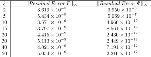
Tables10-12displays the (LSPM) residual error forF,ΘandΦ respectively. It can be seen from the tables that the saturation level is at least10−9in the equation forF(η, ξ),10−12in the equationΘ(η, ξ)and at10−12_{in the equation}_Φ(_{η, ξ}_{). This shows that even when}_ξ_{is very}

large, very accurate results can be obtained which is in contrast with the existing (SPM) known in the literature.

5. CONCLUSIONS

In this paper, we have discussed the application of the large parameter spectral perturbation method (LSPM) on systems of nonlinear PDEs. The large parameter spectral perturbation method (LSPM) is used to solve the equations describing the effect of hall current on the MHD laminar nat-ural convection flow from a vertical permeable flat with uniform surface temperature, free convection from a vertical permeable circular cone with a non-uniform surface, and free convection from a vertical permeable circular cone with non-uniform surface heat flux previously investigated bySaha et al.(2007),Hossain and Paul(2001a) andHossain and Paul (2001b), respectively. The purpose of the present study is to present a compliment of the existing spectral perturbation method that solves fluid mechanics problems with large parameters. Also, we have been able to show that the range of validity of the standard spectral perturbation method (SPM) can be extended by expanding about a large physical pa-rameter so as to make the standard (SPM) robust, efficient and extend its application to new areas. From the numerical simulations, some conclu-sions can be drawn as follows;

• The results become more accurate even asξbecomes larger. This observation contradicts the standard (SPM) which does not give accurate results asξapproaches1. We remark also that very few terms of the (LSPM) is required to obtain converged results pre-sented in the Tables.

• Significantly few seconds was required to attain desired converged results that are comparable with published literature. The compu-tational speed of our approach is primarily due to the fact that with the spectral collocation method, only few grid points are required to yield accurate results. Hence, it is concluded from the observa-tions made that the (LSPM) is computationally fast.

• The (LSPM) can be used as an alternative numerical approach to get numerical solutions for higher order asymptotic series equa-tions that are not possible to find, or very difficult to find with the usual asymptotic perturbation schemes.

• The ease of implementation, computational speed and accuracy of the (LSPM) suggest that this method can be used to extend the range of validity of the standard (SPM), and improves the conver-gence rate of the usual (SPM) even asξbecomes larger in as much the series expansion is about a large parameter.

(12)

DOI: 10.5098/hmt.9.36 ISSN: 2151-8629

Table 10LSPM residual error for Equations (1-3) at different values ofξwhenm= 100,P r= 0.7,M = 0.5,L= 40, andNx= 60

ξ ||Residual Error F||∞ ||Residual ErrorΦ||∞

2 2.850×10−4 3.865×10−3 5 2.747×10−9 ₆_.₁₁₀_×₁₀−11

10 3.212×10−9 1.472×10−12 15 2.640×10−9 ₆_.₁₆₈_×₁₀−12

20 2.805×10−9 3.240×10−12 30 2.922×10−9 4.349×10−12 40 2.640×10−9 ₂_.₈₉₉_×₁₀−12

50 3.237×10−9 1.727×10−12

Table 11LSPM residual error for Equations (6-7) at different values ofξwhenn= 0.5,P r= 0.7,L= 40, andNx= 60

2 9.391×10−3 9.536×10−3 5 2.915×10−9 3.448×10−6 10 3.227×10−9 ₁_.₃₅₅_×₁₀−8

15 2.363×10−9 5.287×10−10 20 3.881×10−9 ₅_.₂₉₁_×₁₀−11

30 3.261×10−9 3.581×10−12 40 2.956×10−9 2.685×10−12 50 2.952×10−9 ₄_.₂₀₆_×₁₀−12

Table 12LSPM residual error for Equations (10-11) at different values ofξwhenm= 0.5,P r= 0.7,L= 40, andNx= 60

2 3.619×10−5 ₃_.₉₅₀_×₁₀−3

5 5.434×10−9 5.069×10−7 10 3.571×10−9 4.960×10−10 15 3.797×10−9 ₈_.₅₆₁_×₁₀−12

20 4.415×10−9 2.430×10−12 30 5.113×10−9 ₂_.₄₄₉_×₁₀−12

40 4.021×10−9 7.191×10−12 50 5.054×10−9 2.216×10−12

ACKNOWLEDGMENT

The authors wish to thank the University of KwaZulu-Natal and DST-NRF Centre of Excellence in Mathematical and Statistical Sciences (CoE-MaSS), South Africa for necessary support.

REFERENCES

Agbaje, T.M., Motsa, S.S., 2015 “Comparison between Spectral Pertur-bation and Spectral Relaxation Approach for Unsteady Heat and Mass Transfer by MHD Mixed Convection Flow over an Impulsively Stretched Vertical Surface with Chemical Reaction Effect,”Journal of Interpola-tion and ApproximaInterpola-tion in Scientific Computing2015, (1), 48–83. http://doi:10.5899/2015/jiasc-00076

Bhattacharyya, K., 2013, “Boundary Layer Stagnation-Point Flow of Casson Fluid and Heat Transfer Towards a Shrinking/Stretching Sheet,” Frontiers in Heat and Mass Transfer4, 1–9, Article ID 023003. http: //dx.doi.org/10.5098/hmt.v4.2.3003

Chamkha, A.J., Takhar, H.S., Nath, G., 2003, “Unsteady MHD Rotating Flow over a Rotating Sphere near the Equator,”Acta Mechanica164, (1– 2), 31–46.

https://doi.org/10.1007/s00707-003-0011-z

Canuto, C., Hussaini, M.Y., Quarteroni, A., Zang, T.A., 1988, “Spectral Methods in Fluid Dynamics,”Springer-Verlag, Berlin.

https://doi.org/10.1007/978-3-642-84108-8

Gorla, R.S.R., Slaouti, A., Takhar, H.S., 1998, “Free Convection in Mi-cropolar Fluids over a Uniformly Heated Vertical Plate,” International Journal Numerical Methods for Heat & Fluid Flow8, (5), 504–518. https://doi.org/10.1108/09615539810220261

Hossain, M.A., Paul, S.C., 2001, “Free Convection from a Vertical Per-meable Circular Cone with Non-uniform Surface Temperature,” Acta Mechanica151, (1–2), 103–114.

https://doi.org/10.1007/BF01272528

Hossain, M.A., Paul, S.C., 2001, “Free Convection from a Vertical Per-meable Circular Cone with Non-uniform Surface Heat Flux,”Heat and Mass Transfer37, (2–3), 167–173.

https://doi.org/10.1007/s002310000129

Hussain, S., Hossain, M.A., Wilson, M., 2000, “Natural Convection Flow from a Vertical Permeable Flat Plate with Variable Surface Temperature and Species Concentration,” Engineering Computations 17, (7), 789– 812.

https://doi.org/10.1108/02644400010352261

Motsa, S.S., Magagula, V.M., Sibanda, P., 2014, “A Bivariate Cheby-shev Spectral Collocation Quasilinearization Method for Nonlinear Evo-lution Parabolic Equations,”The Scientific World Journal2014, Article ID 581987, 13 pages.

http://dx.doi.org/10.1155/2014/581987

(13)

Variable Thermal Conductivity,”Thermal Science19, (1), 239–248. https://doi.org/10.2298/TSCI15S1S39M

Oyelakin, I.S., Mondal, S., Sibanda, P., 2017, “Unsteady MHD Three - dimensional Casson Nanofluid Flow over a Porous Linear Stretching Sheet with Slip Condition,”Frontiers in Heat and Mass Transfer837, 1–9.

DOI: 10.5098/hmt.8.37

Roy, S., Takhar, H.S., Nath, G., 2004, “Unsteady MHD Flow on a Rotat-ing Cone in a RotatRotat-ing Fluid,”Meccanica39, (3), 271– 283.

https://doi.org/10.1023/B:MECC.0000022847.28148.98

Saha, L.K., Hossain, M.A., Gorla, R.S.R., 2007, “Effect of Hall Current on the MHD Laminar Natural Convection Flow from a Vertical Perme-able Flat Plate with Uniform Surface Temperature,”International Journal of Thermal Sciences46, (8), 790–801.

https://doi.org/10.1016/j.ijthermalsci.2006.10.009

Slaouti, A., Takhar, H.S., Nath, G., 2002 “Spin-up and Spin-down of a Viscous Fluid over a Heated Disk Rotating in a Vertical Plane in the Presence of a Magnetic Field and a Buoyancy Force,”Acta Mechanica

156, (1–2), 109–129.

https://doi.org/10.1007/BF01188745

Takhar, H.S., Chamkha, A.J., Nath, G., 2001, “Unsteady Three-dimensional MHD-boundary-layer Flow due to the Impulsive Mo-tion of a Stretching Surface,” Acta Mechanica 146, (1–2), 59–71. https://doi.org/10.1007/BF01178795

Takhar, H.S., Nath, G., Singh, A.K., 2001,“Unsteady MHD Boundary-layer of a Source and Vortex Flow Adjacent to a Stationary Surface,” Acta Mechanica146, (1–2), 9–20.

https://doi.org/10.1007/BF01178791