________________________________
* Corresponding Author. Email: [email protected]
USING INCOMPLETE VARIABLE CROSS-SECTION HIGHLY
CONDUCTIVE INSERTS FOR COOLING A DISC
F. Sharifi
a, H. Ghaedamini
b,*M.R. Salimpour
aa
Department of Mechanical Engineering, Isfahan University of Technology, Isfahan 84156-83111, Iran
b Department of Mechanical Engineering, National University of Singapore, 9 Engineering Drive 1, Singapore 117576, Singapore
A
BSTRACTIn the present study, conductive cooling of a disc is done by means of incomplete constant and variable cross-section highly conductive inserts embedded in radial and tributary configurations. Variational calculus is invoked to determine the optimum shape of the cross-sections of the inserts. Firstly, it is tried to derive an equation for thermal resistance of the disc for radial configuration of inserts based on the procedure used in constructal studies. This is done by implementing the optimized thermal resistances of elemental sectors. Then, the computed elemental sectors are put together so that they make branching configuration of inserts in the disc. Out of the comparison between the obtained thermal resistances of the disc with constant and variable cross-sections, it is concluded that using variable cross-sections reduces thermal resistance, but this effect differs in radial and tributary configurations, i.e., increasing the complexity of tributary patterns does not always reduce the thermal resistance more effectively in comparison with radial configurations.
Keywords: Constructal, variable cross-section, variational, incomplete insert, disc, cooling.
1. INTRODUCTION
In today’s high-performance microelectronics, one can say for sure that heat dissipation is among the important factors that need special attention as in some cases it acts as a bottleneck which dictates the performance of the system. Moreover, as the length scale of these devices continues to diminish, convective cooling of the component may not be viable due to technical issues. Therefore, conduction of the heat by means of highly conductive inserts emerges as a tool to transfer the generated heat to the edge or the center of the device where attached heat sink can be used to remove this heat. This method is used in this paper for cooling a disc shape body based on constructal theory.
Constructal theory attempts to explain the evolvement of finite-size flow systems through time and it says this evolvement is based on a simple law: for a finite size flow system to survive in time, it should evolve in such a way that it provides easier access to the flow that goes through it. Knowing this law, one not only can explain natural systems but also he can implement it into man-made devices as an attempt to reach to the designs that are more natural, keeping in mind that nature has the answer to lots of our problems. Here, it should be noted that even the natural systems are not duly perfect. Hence, the future does not belong to the perfect, or the ideal, but it belongs to the imperfect designs that are the least imperfect possible (Bejan and Lorente, 2008). This has been the time arrow of design evolution in technology, biology, geomorphology, and social organization in the past years (Bejan, 2000, 2008, 2010; Bejan et al., 2000; Bejan and Lorente, 2006; Bejan and Merkx, 2007).
Pure conductive cooling of electronic components by using highly conductiveinserts implemented in low conductivedomain is one applicable area of constructal theory which many aspects of it are investigated until now. Ledezma et al. (Ledezma et al., 1997) constructed a cooling network for a rectangular domain with constant
volumetric heat generation. They concluded that a tree-shaped network of highly conductive material should be an optimum design. Dan and Bejan (Dan and Bejan, 1998) looked into the problem from a different angle and by changing the geometry of flow path, they tried to minimize the time needed to discharge a volume to a sink by means of a constructal tree network. Almogbel and Bejan (Almogbel and Bejan, 2001) used non-uniform distribution of highly conductive material. By this configuration, they could achieve a significant improvement in global performance. Mathieu-Potvin and Gosselin (Mathieu-Potvin and Gosselin, 2007) proposed an evolutionary algorithm to optimize the thermal resistance and by comparing their results to those predicted previously by constructal theory, they showed several similarities in term of performances and geometries. Gosselin and Bejan (Gosselin and Bejan, 2004) studied tree configuration of highly conductive materials at micro and nano scales and stated that at such a small scale, thermal conductivities vary with the shape and dimension of the system. All of the above works were done for a rectangular domain; however, there are also some investigations for circular (Rocha et al., 2002, 2006) and triangular (Ghodoossi and Egrican, 2004) domains. An analytical solution for radial and bifurcation configuration of highly conductive inserts embedded in a disc was presented by Rocha et al. (Rocha et al., 2002). They believed that highly conductive material inserts can change the direction of heat flux into two perpendicular directions. A later work by Rocha et al. (Rocha et al., 2006) was devoted to a different construction by adding loops to the configuration.
There is a series of studies in which the widths of inserts are optimized using variational calculus. Ledezma et al. (Ledezma et al., 1997) used cross-sectional optimized inserts to minimize resistance of the tree network. Then Rocha et al. (Rocha et al., 2002) utilized this method to optimize the width of radial inserts distributed in a disc domain and further compared thermal resistance and other geometric parameters related to this case to a constant-D assumption.
Frontiers in Heat and Mass Transfer
2
Optimizing of variable cross-section highly conductive insert was developed in refs. (Wei et al., 2009; Wei et al., 2010; Zhou et al., 2007) for a rectangular domain. In these investigations based on constructal theory, the thermal resistance was optimized through assembling the constructs in several times using the results of the simpler elemental constructs. Comparison of the results was done in each step by comparing them with simpler architectures with fewer assemblies (Zhou et al., 2007) and also with constant cross-section configurations (Wei et al., 2009). Mentioned results revealed that increasing the complexity of the configuration cannot always decrease the thermal resistance. However it is mentioned that the optimized minimum thermal resistance of variable cross-section cases is smaller than that of constant cross-section. The recent study performed by using constructal entransy dissipation rate minimization method based on discrete variable cross-section highly conductive insert (Wei et al., 2010) showed that as the assembly’s order increases, i.e. complexity of the architecture, the minimum mean temperature difference on elemental area with variable cross-section highly conductive insert increases whereas for the case of constant cross-section highly conductive insert, this parameter decreases and for both of them, it approaches a constant as the assembly’s order increases.
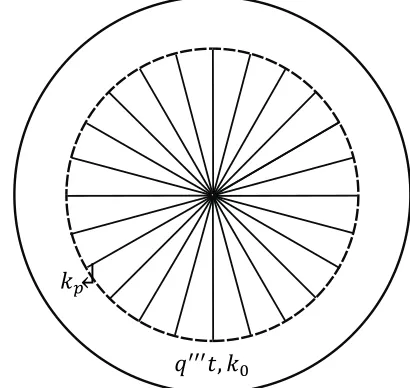
In the present study, the work on incomplete inserts extending outward from center to a specific distance in a disc (Fig. 1) is further developed by giving another degree of freedom to the geometry; that is, the cross-section change of inserts. By using variational calculus, the incomplete variable cross-section highly conductive inserts in radial and branching configurations used for cooling a disc-shaped body are investigated. Hence, the optimized thermal resistance is determined and compared to the constant cross-section highly conductive insert case. The results showed that for the case under study here, decrease of thermal resistance can be achieved from the case with constant cross section inserts. Moreover, under some circumstances which will be illustrated, the thermal resistance of the disc with incomplete inserts surpasses the complete insert structure. Also by increasing the complexity of the network from radial to branching configurations, there is less decrease in optimized thermal resistance. That means increasing the complexity of the system will diminish the effect of varying cross-section on thermal resistance. However, it should be noted that this is an achievement itself as the price of highly conductive material is a determining factor.
2. DESCRIPTION OF THE PROBLEM
Designing a disc-shaped electronic component is considered in this study, Fig. 1. In an analogy to constructal studies, we should define the constraints as well as degrees of freedom; these two will compete against each other to shape the geometry. Usually, global constraint is the volume occupied by the device and in this way, installing as much circuitry as possible in this volume should be the objectiveof the design. Since from the thermal design point of view, the pure effect of these components is the heat generation, the objective simply means as much heat generation as possible in this specified volume. The local constraint is to prevent the highest temperature of the package, Tmax, exceeding a specified value. It is obvious that if
Tmax goes beyond this allowable amount, the function of the local component is threatened. Without any major effect on the generality of the problem and just for the sake of simplicity, it is considered that there is a uniform distribution of heat generation throughout the adiabatic wall bounded disc. To gather heat, highly conductive inserts with the thickness of 𝐷 are implemented which their material’s conductivity, kp, is considerably higher than the disc’s material with conductivity of k0 such that 𝑘�=𝑘𝑝/𝑘0≫1. This
network of highly conductive inserts then derives the heat to the center of the disc where a heat sink exists to gather that heat. Figure 1 shows a radial configuration of the inserts. The composition of the two-material composite is fixed which is accounted for by defining volume fraction 𝜙 as the volume of kp material to total volume.
Fig. 1 Incomplete radial configuration of highly conductive inserts embedded in a uniform heat generating disc.
3. MATHEMATIC FORMULATION
In this part, using variational calculus, cross-section of the highly conductive insert for radial configuration is optimized and then considering the calculated cross-section shape, it is tried to optimize the thermal resistance. Similarly, the same procedure is implemented for the fractal network. Also, the relation of constant cross-section highly conductive insert is compared with that of variable cross-section highly conductive insert.
3.1. Radial pattern
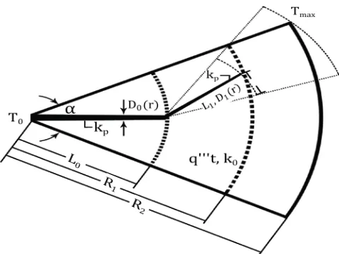
A radial configuration is maybe the simplest structure to design a conductive network to cool a disc. The disc with radial inserts, Fig. 1, is composed of 𝑁 sectors which are shown in Fig. 2.
Fig. 2 A sector of the disc with radial variable cross section configuration of highly conductive material.
𝑞
′′′𝑡
,
𝑘
0↲
3
It is assumed that there are many radial inserts so that the sectors are slender enough to be approximated by an isosceles triangles of base
2𝐻 and height 𝑅.
20B
At first, based on the constructal theory, one of these sectors is considered as the elemental volume. Then, its thermal resistance is determined and optimized due to various aspect ratios. The corresponding thermal resistance of the entire disc can be calculated by assembling the sectors together.
21B
As the inserts are considered incomplete, there is a region in the disc where there is no highly conductive insert in it. Thus, the domain can be divided into two regions: the outer region without highly conductive inserts and the central part with the cooling inserts.
22B
3.1.1. Region without highly conductive material
23B
Firstly, bear in mind that there is no difference in formulating thermal resistance between constant and variable cross-section highly conductive insert for the outer region where there is no cooling insert. Two-dimensional conduction equation in cylindrical format can be written as,
𝜕2𝑇 𝜕𝑟2+
1 𝑟 𝜕𝑇 𝜕𝑟+ 1 𝑟2 𝜕2𝑇 𝜕𝜃2+
𝑞′′′ 𝑘0 = 0
(1)
24B
In order to solve the above equation, boundary conditions should be specified. As the disc is adiabatic, there is no heat conduction at the edge and (𝜕𝑇𝜕𝑟)(𝑟=𝑅2,𝜃)= 0, also ( 1𝑟𝜕𝑇𝜕𝜃)(𝑟,𝜃=0)= 0
and ( 1 𝑟
𝜕𝑇
𝜕𝜃)(𝑟,𝜃=𝛼)= 0 due to symmetry of the problem where 𝜃0 is the sectional degree. Since highly conductive material is responsible for the main part of the heat flux conduction, it is approximated that the direction of the heat flux at 𝑟 ≤ 𝑅1 is perpendicular to the insert. Thus, 𝑇(𝑟=𝑅1,𝜃)≈ 𝑓(𝜃) is the fourth boundary condition. It should be noted that this assumption is also implemented in (Rocha et al., 2002) to obtain the temperature difference between the heat sink and the highly conductive inserts connected to the rim of the disc. Moreover, in section 4.3, consistency of this assumption is checked by solving the problem numerically in a 2D format. Comparing the results of numerical and analytical solutions, similar behavior and acceptable agreement between them are observed.
25B
With the above boundary conditions, using change of variables to homogenize the equation, then separating variables and finally nondimensionalizing the maximum temperature difference, it can be concluded that,
𝑇�1=Tqmax′′′A1−/kT00=
1 3
𝐻1 𝑅1−
�4((𝑛𝜋−1))2𝑛[ (𝑅2/𝑅1)𝜆𝑛 1 + (𝑅2/𝑅1)2𝜆𝑛]
𝐻1 𝑅1 ∞
𝑛=1
−14��𝑅2𝑅1�2−1�𝑅1𝐻 1
+12�𝑅𝑅12�2𝑙𝑛 �𝑅𝑅12�𝐻1𝑅1 (2)
26B
where 𝐴1=𝐻1𝑅1 and 𝜆𝑛=𝑛𝜋/𝛼 are the characteristic values.
27B
3.1.2. Region with highly conductive material
28B
In order to analyze conduction along the kpblade in this region, first notice that the heat current which flows toward the center increases from 𝑞= 0 at 𝑟=𝑅2 to the total current of 𝑞=𝑞′′′𝑡𝐴 at 𝑟= 0; where 𝑞′′′ is the volumetric heat generation, 𝐴 is the total area of the disc and 𝑡 is the thickness of the disc. The increase experienced by 𝑞 at an intermediate position, 𝑟, is,
−𝑑(𝑞) =ℎ𝑞′′′𝑡𝑑𝑟 (3)
29B
Where ℎ𝑞′′′𝑡 is the amount of heat current gathered over the vertical surface ℎ𝑡 and ℎ= (𝐻1/𝑅1)𝑟 considering an isosceles
triangle to represent the sector. The relation between heat and local temperature gradient is,
𝑞=𝑘𝑝𝐷2𝑡𝑑𝑇𝑑𝑟 (4)
30B
Eliminating 𝑞 between Eqs. (3) and (4) we encounter a second order differential equation with following boundary conditions,
𝑇=𝑇0 𝑎𝑡 𝑟= 0 (5)
𝑞′′′𝜋(𝑅 2 2− 𝑅
12)𝑡
2𝑁 =𝑘𝑝𝐷2𝑡𝑑𝑇𝑑𝑟 𝑎𝑡 𝑟=𝑅1 (6)
31B
Now two different cases can be pursued: constant and variable cross-section inserts. For the constant cross-section, D = cte, the resultant second order differential equation can be integrated twice and by invoking boundary conditions, Eqs. (5) and (6), specifying 𝑇=𝑇𝑅1 at 𝑟=𝑅1 and nondimensionalizing the temperature difference between 𝑇𝑅1and 𝑇0 , it can be concluded that,
𝑇�2(𝑐𝑡𝑒) =𝑞𝑇𝑅′′′1𝐴1− 𝑇0/𝑘0=
1
𝑘�𝜙� 𝑅1 𝑅2�
2 �𝑅𝐻1
1� �� 𝑅2 𝑅1�
2
−13� (7)
32B
For the variable cross-section highly conductive insert, 𝐷=𝐷(𝑟), by integrating twice from the differential equation: 𝑇𝑅1− 𝑇0=� 𝐷𝐴(𝑟)𝑑𝑟
𝑅1
0
(8)
33B
where
𝐴=−𝑘2
𝑝�𝑞 ′′′𝑟2
2
𝐻1
𝑅1+𝑐1� 𝑤ℎ𝑒𝑟𝑒𝑐1: 𝑐1= − �𝑞
′′′𝜋(𝑅 2 2− 𝑅
1 2)
2𝑁 +
𝑞′′′(𝐻1𝑅1)
2 � (9)
34B
Also the volume fraction of highly conductive material to the whole sector is,
𝜙=𝐻2𝑅21 � 𝐷𝑅1 (𝑟)
0 𝑑𝑟
(10)
35B
It is noted that 𝜙 is the constraint of the problem. Using variational calculus, function of 𝐷(𝑟) can be determined with respect to this constraint, Eq. (10), such that Eq. (8) is optimized,
𝐷(𝑟) =𝑐[(𝑅1)2−(𝑟)2] 1
2 (11)
36B
Substituting Eq.(11) into constraint (10), the constant factor 𝑐 can be computed and we will have,
𝐷(𝑟) = 2𝜙1𝐻1(𝑅1/𝑅2)2
�(𝑅1/𝑅2)�1−(𝑅1/𝑅2)2+ sin−1(𝑅1/𝑅2)�
× [(𝑅2/𝑅1)2−(𝑟/𝑅1)2]12 (12)
37B
Which 𝜙=𝑁𝜋𝑅𝐷𝑅1 22 =𝜙1 �
𝑅1 𝑅2�
2
and when 𝑅1/𝑅2 approaches to
unity, i.e. a complete insert, the result will become equal the one reported in [14] as,
�𝐷(𝑟)�𝑐𝑜𝑚𝑝𝑙𝑒𝑡𝑒𝑖𝑛𝑠𝑒𝑟𝑡=4𝜋 𝜙𝐻[1−(𝑟/𝑅)2]12 (13)
38B
Similar to the procedure implemented for constant-D
assumption, The thermal resistance is calculated by substituting Eq. (12) into Eq. (8) and nondimensionalizing it,
𝑇�2(𝑣𝑎𝑟𝑖𝑎𝑏𝑙𝑒)=qT′′′𝑅1A−1/kT00=
1 4𝑘�𝜙1�
𝑅2 𝑅1�
4 �𝑅1𝐻
1�
×��𝑅1𝑅2� �1− �𝑅1𝑅2�2+ sin−1�𝑅1 𝑅2��
2
(14)
39B
4
(𝐻1/𝑅1) provided other parameters are kept constant. Thus,
(𝐻1/𝑅1)𝑜𝑝𝑡 is the value at which optimum thermal resistance occurs. Finally, The corresponding thermal resistance of the entire disc is obtained by using 𝐴𝑑𝑖𝑠𝑐 instead of 𝐴1 in Eqs.(2) and (7),
𝑇�𝐺𝑅,𝑜𝑝𝑡=𝑞𝑇′′′𝑚𝑎𝑥𝜋𝑅− 𝑇0 2 2/𝑘
0=� 𝑇� 𝜋� �
𝑅1 𝑅2�
2 �𝐻1𝑅1�
𝑜𝑝𝑡
(15)
3.2. Fractal pattern
Now, we consider the elemental construct of a fractal network of highly conductive structure as shown in Fig. 3. To design tree-shaped incomplete inserts, the results derived for radial configuration will be benefited from. It is noticeable that as the boundary conditions for the stem are different, the result of section 3.1 cannot be used directly for the total fractal configuration. Thus, the domain should be divided into two major parts: the most outer region where there is no highly conductive insert plus the region where tributaries are embedded in and the central part where the insert’s configuration is radial. Fig. 3 shows these three regions with three concentric circle slices.
Fig. 3 A sector of the disc with branching variable cross section configuration of highly conductive material.
3.2.1. Outer region
As was mentioned previously, derived formula for calculating thermal resistance for radial configuration can be used for this region. Only keep in mind that some notations need to be changed as the region boundaries are different in this case. Thus, to express the thermal resistance of outer region using the radial configuration result, beneath changes are to be done in the notations,
𝑅1(𝑠𝑒𝑐𝑡𝑖𝑜𝑛 3.1)→ 𝐿1(ℎ𝑒𝑟𝑒), 𝐷/2→ 𝐷1/2, 𝑇0→ 𝑇𝑐,
𝑅2→(𝑅2− 𝑅1+𝐿1) (16)
Thus, (H1/R1) is replaced by (H1/L1), and the following relations for the portion between L0 and R2 can be used,
�𝐻1𝐿1�=�𝐻𝐿11� 𝑜𝑝𝑡
(𝑠𝑒𝑐𝑡𝑖𝑜𝑛. 3.1),
𝜙1=𝐷1𝐻1,𝐴1=𝐻1𝐿1 (17)
As the result, 𝐷1(𝑟) would be,
𝐷1(𝑟) = 2𝜙1𝐻1(𝐿1/𝑀)2
�(𝐿1/𝑀)�1−(𝐿1/𝑀)2+ sin−1(𝐿1/𝑀)�
[(𝑀/𝐿1)2−(𝑟/𝐿1)2]12 (18)
where 𝑀 ≡ 𝑅2− 𝑅1+𝐿1, and (𝑀/𝐿1) is,
�𝐿𝑀
1�= 1 +� 𝑅2 𝐿1� − �
𝑅1 𝐿1�
= 1 +𝑅�1�𝐻1𝐿1� 𝑜𝑝𝑡 1 2
��𝑅2𝑅1� −1� (19)
Applying above notations in the equation derived previously in section 3.1, the thermal resistances corresponding to both regions, the one without highly conductive inserts plus region with tributary part, for constant and variable cross-section inserts are expressed by Eqs. (20) and (21), respectively.
𝑇�1(𝑐𝑡𝑒)=𝑇𝑞𝑚𝑎𝑥′′′𝐴− 𝑇𝑐 1/𝑘0 =
1 3
𝐻1 𝐿1− �
4(−1)𝑛
(𝑛𝜋)2 [ (𝑀/𝐿1) 𝜆𝑛 1 + (𝑀/𝐿1)2𝜆𝑛]
𝐻1 𝐿1 ∞
𝑛=1
−14��𝑀𝐿1�2−1�𝐻1𝐿1+12�𝐿1𝑀�2𝐻1𝐿1𝑙𝑛 �𝐿1𝑀�
+ 1
𝑘�𝜙1� 𝐿1 𝐻1� ��
𝑀 𝐿1�
2
−13� (20)
𝑇�1(𝑣𝑎𝑟𝑖𝑎𝑏𝑙𝑒)=𝑇𝑞𝑚𝑎𝑥′′′𝐴1− 𝑇/𝑘0𝑐=
1 3
𝐻1 𝐿1− �
4(−1)𝑛
(𝑛𝜋)2 [
(𝑀/𝐿1)𝜆𝑛
1 + (𝑀/𝐿1)𝜆𝑛] 𝐻1 𝐿1 ∞
𝑛=1 −14��𝑀𝐿
1� 2
−1�𝐿1𝐻 1+
1 2�
𝑀 𝐿1�
2𝐿1 𝐻1𝑙𝑛 �
𝑀 𝐿1�
+ 1
4𝑘�𝜙1� 𝐿1 𝐻1� �
𝑀 𝐿1�
4
×��sin−1�𝐿1 𝑀��+�
𝐿1 𝑀�(1− �
𝐿1 𝑀�
2
)1/2� 2
(21)
3.2.2. Central part
As the boundary conditions for this part are different, we cannot use
(𝐻1/𝐿1 )𝑜𝑝𝑡 for the (𝐻0/𝐿0 ) obtained from section 3.1; instead, it can be written as,
�𝐻𝐿00� ≅ �𝛼2�, 𝐴0=𝐻0𝐿0 (22)
where 𝛼 is the tip angle (Fig. 2) which is the function of other geometric parameters, i.e. the number of 𝐿1 or 𝐴1 elements, N, and the number of branches 𝐿1 which is connected to the radial inserts, n. thus,
𝛼=2𝑁𝜋𝑛=2𝜋𝑅12𝜋𝑛/2𝐻1=2𝑛
𝑅�1� 𝐻1 𝐿1�𝑜𝑝𝑡
1/2
(23)
In Eq. (23), 𝑅�1≡ 𝑅1/𝐴11/2 and the area 𝐴0 of the central sector is,
𝐴0≅ 𝑛𝑅�1�𝐻1𝐿 1�𝑜𝑝𝑡
1/2
𝐴1�1−𝑅�1 1�
𝐻1 𝐿1�𝑜𝑝𝑡
−1/2 �
2
(24)
Again, two scenarios can be considered for the cross-section, i.e. variable and constant. In the case that 𝐷0 and 𝐷1 are assumed constant, the temperature difference between 𝑇𝑐 and 𝑇0 is determined by eliminating q between Eqs. (3) and (4), then integrating twice from the resultant differential equation, invoking 𝑇=𝑇0 at 𝑟= 0 and another boundary condition from the radial pattern which is,
𝑘𝑝𝐷0(𝐿0)𝑡 �𝑑𝑇𝑑𝑟�𝑟=𝐿 0
≅ 𝑞′′′𝑡 �𝑛𝐴1+�𝛼
5
This boundary condition expresses that the heat generated in the outer region is gathered and transformed to the heat sink in the center by means of stem embedded in the central region. The temperature difference for constant-D assumption is then nondimensionalized and as specified before, 𝑇=𝑇𝑐 at =𝑅1; hence,
𝑇�2(𝑐𝑡𝑒)=𝑞𝑇′′′𝑐𝐴− 𝑇1/𝑘00=
�𝑅�1− �𝐿1 𝐻1�𝑜𝑝𝑡
1/2 � 𝑘�𝜙1𝐷� �
𝐿1 𝐻1�𝑜𝑝𝑡
1/2
× [23𝑛𝑅�1�𝐻1𝐿1� 𝑜𝑝𝑡 1/2
�1−(𝐿1/𝐻1)𝑜𝑝𝑡 1/2
𝑅�1 �
2
+𝑛+𝑛𝑅�1�𝐻1𝐿1� 𝑜𝑝𝑡 1/2
×��𝑅2𝑅 1�
2
−1�] (26)
For variable cross-section highly conductive insert, after integrating twice from the differential equation and invoking above boundary conditions, we have,
𝑇(𝑟)− 𝑇0=� 𝑘 −1 𝑝𝐷0(𝑟)��
𝐻0 𝐿0� 𝑞
′′′𝑟2+𝑐 1� 𝑑𝑟 𝑟
0 ,
𝑐1=−𝑞′′′��𝐻0
𝐿0�(𝑅22− 𝑅12) +𝑛𝐴1+𝐴0� (27) Again, volume fraction is the constraint,
𝜙= 𝐴𝑝
𝜋𝑅22
= 1
𝜋𝑅22�𝑁 � 𝐷1(𝑟) 𝐿1
0 𝑑𝑟+ (𝑁/𝑛)� 𝐷0(𝑟)𝑑𝑟 𝐿0
0 �
(28)
Relation for 𝜙 can be improved further as,
𝜙=�𝐻1𝐿1�1/2𝑅�1(−1)�𝑅2𝑅1� 2
𝜙1
+�𝐻𝐿1 1�
1/2 𝑅�1�𝑛𝑅1
22� � 𝐷0(𝑟)𝑑𝑟, 𝐿0
0 𝜙1=𝐻1
1𝐿1� 𝐷1(𝑟) 𝐿1
0 𝑑𝑟
(29)
Now, optimizing Eq. (27) regarding to Eq. (29), we have, 𝐷0(𝑟) =
�𝐶1𝐶22 � �𝑅2𝑅1�2(𝜙 − 𝐶3𝜙1)𝐻0 𝐶42 �𝐶4
2− �𝑟 𝐿0�
2 �
1/2
(30)
where
𝐶1= sin−1(1/𝐶4) + (1/𝐶4)�1−(1/𝐶4)2,
𝐶2=�1−𝑅�1 1�
𝐿1 𝐻1�
1/2 �
2
,𝐶3=𝑅�1 1�
𝐿1 𝐻1�
1/2 �𝑅1𝑅
2� 2
,
𝐶4=�1 +𝑅�1 1𝐶2�
𝐿1 𝐻1�
1 2
+𝐶1
2�� 𝑅2 𝑅1�
2 −1��
1/2
(31)
Substituting Eq. (30) into Eq. (27) and nondimensionalizing it, the thermal resistance for this region can be expressed as,
𝑇�2(𝑣𝑎𝑟𝑖𝑎𝑏𝑙𝑒)=𝑞𝑇′′′𝑐𝐴1− 𝑇/𝑘00
=�2𝛼� �𝑅1𝑅2�2 𝐶1𝐶2𝐶42
2𝑘�(𝜙 − 𝐶3𝜙1)×
[�𝑅�12�𝛼2� �𝑅𝑅2 1�
2
�1− �𝑅𝑅1 2�
2
�+𝑛�sin−1�1 𝐶4�
+�𝐴0𝐴1� �sin−1(1/𝐶4)− �𝐶42
2� 𝐶1∗�] (32)
where 𝐶1∗ is the conjugate of 𝐶1.
Furthermore, the global thermal resistance for branching pattern, 𝑇�𝐺𝐵,𝑜𝑝𝑡, can be written as,
𝑇�𝐺𝐵,𝑜𝑝𝑡=𝑞𝑇′′′𝑚𝑎𝑥𝜋𝑅− 𝑇0 22/𝑘0=�
𝑇� 𝜋𝑅�12� �
𝑅1 𝑅2�
2
(33)
4. RESULT AND DISCUSSION
Thermal resistance of radial and fractal configurations are analyzed in this section. For each structure, more attention is paid to the width of the highly conductive insert cross-section. Moreover, the thermal resistance of variable cross-section is compared with that of constant cross-section configuration for different conditions. In a nutshell, it is concluded that variable cross-section always decreases the thermal resistance but when the complexity of the control volume increases, the percentage of decrease in thermal resistance diminishes. Worth to mention that even in the latter case, the result is significant in the event that expense of highly conductive material comes to picture.
4.1 Radial pattern
The optimum width of cross-section for radial pattern is obtained using Eq. (12) as a function of the length of the insert keeping other parameters as constants, Fig. 4. This figure is sketched for different 𝑅1/𝑅2 ratios. Since the amount of highly conductive material allocated to the element is assumed to be constant (𝜙=𝑐𝑡𝑒), it is obvious that the mean 𝐷𝑜𝑝𝑡(𝑟) decreases as 𝑅1/𝑅2 increases.
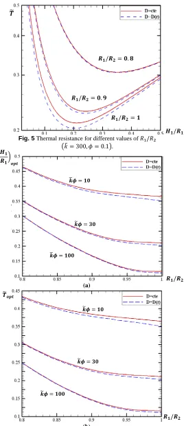
Figure 5 shows the thermal resistance of constant-D and D=D(r)
configurations for different 𝑅1/𝑅2 ratios. A similar behavior can be observed in this figure, i.e. in both cases, constant and variable cross-sections, there is an optimum point due to aspect ratio of the elemental construct, 𝐻1/𝑅1. Also, as 𝑅1/𝑅2 increases, the decrease in thermal resistance is more obvious.
Fig. 4𝐷𝑜𝑝𝑡(𝑟) at different 𝑅1/𝑅2.
Because of the complexity of Eq. (2) plus (7) and Eq. (2) plus (14), it is hard to obtain an analytic relation for optimum thermal resistance. Thus, optimum aspect ratios and optimum thermal resistances are determined by solving the equations numerically as shown in Fig. 6 (a,b). These figures illustrate that the decrease in both of the optimum values intenifies as 𝑅1/𝑅2increases and 𝑘�𝜙 decreases. The reason for this behavior lays in the fact that by increasing the 𝑅1/𝑅2 ratio, the difference between optima of variable
𝒌�𝝓=𝟑𝟎 𝑨𝒆𝒍𝒆𝒎𝒆𝒏𝒕=𝟎.𝟏
6
Fig. 5 Thermal resistance for different values of 𝑅1/𝑅2 �𝑘�= 300,𝜙= 0.1�.
(a)
(b)
Fig. 6 (a) Optimum aspect ratio and (b) optimum thermal resistance for different values of 𝑘�𝜙.
and constant cross-section inserts grows and the increment of 𝑘�𝜙 causes the optimum thermal resistance to become less dependent upon the shape of the inserts. Also, it is clear from Fig. 6 that as 𝑘�𝜙 and 𝑅1/𝑅2 increase, the optimum aspect ratios and thermal resistances decrease, expectedly.
4.1.1. Comparison
In this section, we try to compare the global thermal resistances of configurations with incomplete and complete inserts while cross-section of highly conductive inserts is considered variable. Also, decrease in global resistance by using of variable cross section highly conductive inserts instead of constant one is investigated. Figure 7 shows the percentage of difference in optimum global thermal resistance between complete and incomplete variable cross-section inserts for different 𝑘�𝜙 defined as,
𝛿= 100 ×�IITRCITR−CITR� (34)
where IITR and CITR are incomplete and complete insert thermal resistances, respectively. This figure illustrates that there exists a range of 𝑅1/𝑅2 where the global thermal resistance of incomplete inserts is less than that of complete one; but this range decreases as 𝑘�𝜙 increases. The possible reason is at smaller 𝑘�𝜙s and 𝑅1/𝑅2≈1.0 the cooling power is not efficient enough to change the direction of heat flux considerably to inserts instead of heat sink. Therefore, the optimized condition will be when 𝑅1/𝑅2< 1.0 and as a result, because of the constraint of the problem, the thickness of inserts is proper enough to affect on heat flux, efficiently.
Fig. 7 Difference in optimum global thermal resistance between incomplete and complete inserts �𝐷=𝐷𝑜𝑝𝑡(𝑟)�.
Figure 8 shows the percentage of decrease in optimum global thermal resistance using variable cross-section highly conductive insert defined as,
𝜀= 100 ×�𝑉𝐺𝑅 − 𝐶𝐺𝑅CGR � (35)
where VGR and CGR are global thermal resistances of variable and constant cross-sections, respectively. This figure illustrates that the percentage of decrease rises as 𝑅1/𝑅2 increases and 𝑘�𝜙 reduces. As a matter of fact, 2 factors, 𝑅1/𝑅2 and 𝑘�𝜙, play significant role here. 𝑻�
𝑯𝟏/𝑹𝟏 𝑹𝟏/𝑹𝟐=𝟏
𝑹𝟏/𝑹𝟐=𝟎.𝟖
𝑹𝟏/𝑹𝟐=𝟎.𝟗
𝑹𝟏/𝑹𝟐 𝒌�𝝓=𝟏𝟎
𝒌�𝝓=𝟑𝟎
𝒌�𝝓=𝟏𝟎𝟎
𝑹𝟏/𝑹𝟐 𝑻�𝒐𝒑𝒕
𝒌�𝝓=𝟏𝟎
𝒌�𝝓=𝟑𝟎
𝒌�𝝓=𝟏𝟎𝟎 �𝑯𝑹𝟏
𝟏�𝒐𝒑𝒕
𝟏𝟎𝟎 𝟑𝟎 𝟏𝟎
𝒌�𝝓=𝟑
7
Fig. 8 Difference in optimum global thermal resistance between incomplete inserts; 𝐷=𝑐𝑡𝑒 and 𝐷=𝐷𝑜𝑝𝑡(𝑟).
In small 𝑅1/𝑅2s, with increasing 𝑘�𝜙, the shape of inserts doesn’t change the thermal resistance, considerably. In other words, in small 𝑅1/𝑅2s, the factor of 𝑘�𝜙 has the dominant impact on performance. Furthermore, at this amount of 𝑅1/𝑅2s, the freedom of maneuver is limited and the shape of inserts doesn’t have considerable change, compared with constant D.
In larger 𝑅1/𝑅2s, the shape of inserts has the dominant impact due to the fact that the insert length is stretched enough and its shape is completely different from constant conducting path. In this condition, heat resistance difference corresponding to disc with variable and constant inserts is going to be independent of 𝑘�𝜙.
The maximum percentage of decrease in global thermal resistance is about 7.4 % which occurs at 𝑅1/𝑅2= 1 independently from 𝑘�𝜙.
4.2. Branching pattern
The optimum width of highly conductive insert for stem 𝐷0(𝑟) and tributary 𝐷1(𝑟) which were determined in Eqs. (18) & (30) are plotted in Fig. 9 for different 𝑅�1. This figure illustrates that 𝐿0 increases with 𝑅�1, while 𝐿1 is not so sensible.
Fig. 9 Optimum width of highly conductive inserts for stem 𝐷0(𝑟) and tributary inserts 𝐷1(𝑟) (𝑘�𝜙= 30, 𝑅1/𝑅2= 0.8, 𝐴1= 0.1).
Figure 10 shows the thermal resistance for variable and constant cross-section highly conductive inserts using Eqs. (20), (21), (26) & (32). For all the values of 𝜙1, thermal resistance corresponding to constant D configuration is greater than that of variable cross-section configuration and also they have a behavior similar to the radial pattern.
Fig. 10 Thermal resistance for variable and constant cross-section highly conductive inserts at 𝑘�𝜙= 30, 𝑅1/𝑅2= 0.9.
It is demonstrated from Fig. 10, the thermal resistance has an optimum due to 𝜙1 but because of the complexity of the equation derived for the thermal resistance at section 3.2, the optimum thermal resistance is determined numerically for both cases, constant and variable cross-sections.
As shown in Fig. 11, for two different 𝑘�𝜙s, variable and constant cross-section configurations have a similar trend and both decrease as 𝑅1/𝑅2 increases.
Fig. 11 Optimum thermal resistance for variable and constant cross-section highly conductive inserts at 𝑅�1= 5.
Figure 12 shows the percentage of decrease in optimum global thermal resistance when variable cross-section highly conductive inserts are utilized. This figure illustrates that the decrease in this 𝟑𝟎
𝟏𝟎 𝒌�𝝓=𝟑
𝑹𝟏/𝑹𝟐 𝟏𝟎𝟎
𝑫𝟎(𝒓),𝑫𝟏(𝒓)
𝑫𝟏(𝒓) 𝑫𝟎(𝒓)
𝑹�𝟏=𝟏𝟎 𝑹�𝟏=𝟕
𝑹�𝟏=𝟓 𝑹�𝟏=𝟒
𝒓
𝒌�𝝓=𝟓𝟎
𝒌�𝝓=𝟑𝟎 𝑻�𝒐𝒑𝒕
𝑹𝟏/𝑹𝟐 𝑹�𝟏=𝟓
𝑻�
8
value is less in compare with radial patterns and it is concluded that increasing the complexity of the shape when volume is specified, cannot decrease the optimum global resistance anymore. Moreover, it is evident that the decrement of optimum global thermal resistance increases with 𝑅�1. It is physically logical; in fact, with increasing the dimension of disc, the shape of inserts plays more contribution in reducing the thermal resistance, compared to disc with constant thickness of inserts.
Fig. 12 Decrease in global thermal resistance using variable cross-section highly conductive insert for 𝑘�𝜙= 30.
4.3. Numerical results and comparison
Numerical results presented in this section can be used to validate the analytical solution provided beforehand. Because there is no approximation for the numerical scheme and that the conduction equation is solved in its two dimensional format throughout the whole domain. On the other hand, since the optimum thermal resistances are obtained based on constructal theory, here is a suitable opportunity to examine validity of this strategy. Because, the absolute optimal thermal resistance is obtained here, numerically. Besides, since the speed of numerical method in solving a certain case is considerably less than analytical one, conscientiously thus it is preferred to use the analytical method if there is an acceptable agreement with the numerical one.
There are two different domains to be solved and an interface between them: the region with high conductivity material and the low conductivity region with volumetric heat generation, 𝑞′′′. Thus, the steady state conduction equations for these two different regions can be solved, respectively:
𝑘𝑝∇2𝑇= 0 (36)
𝑘0∇2𝑇=−𝑞′′′ (37)
Because of the symmetry existed in the geometry, a sector of the disc is solved, numerically. 𝜕𝑇/𝜕𝑛= 0 is the boundary condition for all the boundaries except the tip of the sector where a condition of constant temperature is specified which in fact is the temperature of the heat sink. Also, n is the normal vector to each boundary. For the interface, it is assumed that the heat flux is conserved while the temperature is equal for both domains at common nodes.
The equations of 2D conduction are solved numerically using MATLAB partial differential equations toolbox code (MATLAB)
with unstructured triangular elements. The appropriate mesh size is obtained by satisfying the convergence criterion of Eq. (38):
𝛿=�𝑇�𝑚𝑎𝑥 𝑗 − 𝑇�
𝑚𝑎𝑥𝑗+1 𝑇�𝑚𝑎𝑥𝑗
�< 0.001 (38)
where 𝑇�𝑚𝑎𝑥𝑗+1 is the maximum thermal resistance by means of using quadrupled elements relative to 𝑇�𝑚𝑎𝑥𝑗 . Table. 1 shows the results of the above grid study. It is found that refining three steps is enough to satisfy the convergence criterion and the results would be independent from the mesh size.
Table 1 Grid independency test for 𝑅�1= 4, 𝑁= 10.94, 𝑘�= 300, 𝐿�0= 1.98, 𝜙= 0.1, 𝑅1/𝑅2= 0.9 𝑎𝑛𝑑𝐴1= 0.05
Number of elements 𝑇�𝑚𝑎𝑥 𝛿
3720 0.664703 0.001882
14882 0.665954 0.000544
59528 0.666316 0.000178
238112 0.666435
(a)
(b)
Fig. 13 Temperature distribution contours for cases (a) without conductive insert 𝑇�𝑚𝑎𝑥= 26.01 (b) with variable cross-section highly conductive insert 𝑇�𝑚𝑎𝑥= 0.666 at 𝑅�1= 4, 𝑁= 10.94, 𝑘�=
300, 𝐿�0= 1.9767,𝜙= 0.1,𝑅1/𝑅2= 0.9 & 𝐴1= 0.05.
Figure 13 shows the temperature distribution for a sector (a) without highly conductive material (b) with these inserts incompletely distributed through the sector with two branches. The figure demonstrates that there is a considerable decrease in maximum temperature when highly conductive inserts are used which shows the effectiveness of such a cooling system. To compare these results with analytical solution, all of the parameters are non-dimensionalized like section 3.
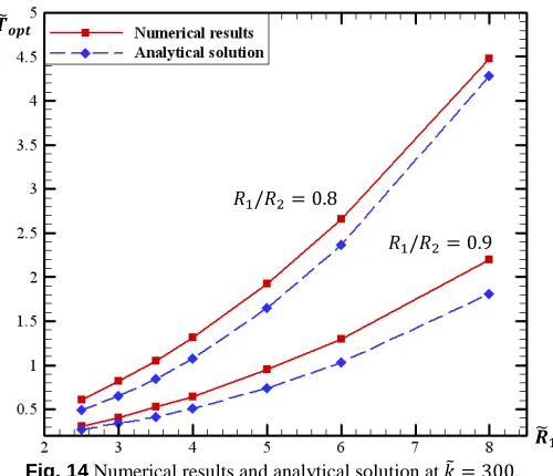
Figure 14 shows a comparison between numerical results and analytical solution for two 𝑅1/𝑅2 cases. This figure portrays similar behaviours for two cases.
𝟏𝟐
𝑹�𝟏=𝟓 𝟖
9
Fig. 14 Numerical results and analytical solution at 𝑘�= 300.
Moreover, it is observed from this figure that there is a good consistency between the results specially for the case with 𝑅1/𝑅2= 0.8. The present difference between the numerical and analytical results are completely logical as in the analytical solution we assumed a one-dimensional conducting equation for the region with highly conductive material. These consistent results present the validity of this assumption and also efficiency of constructal theory in optimizing the flow resistances.
5. CONCLUSION
Incomplete variable cross-section highly conductive networks for radial and tributary configurations are investigated in this paper. The width of inserts is determined using variational calculus. The thermal resistance for constant and variable cross-section cases is solved analytically and it is shown that there is a decrease in thermal resistance for all conditions when variable cross-section inserts are used. But this increase in the complexity of the problem in tributary case is not as effective as in radial configuration in decreasing the thermal resistance. However, incomplete highly conductive inserts in some specific conditions have an advantage over the complete inserts which gives the same and even lower thermal resistance. Finally, as some approximations were used in analytical solution which the most
important of them was the assumption of solving one-dimensional conduction equation for the region with highly conductive material and also the optimization process was carried out based on constructal theory, a numerical solution was performed to validate the analytical results where an acceptable consistency was observed.
NOMENCLATURE
𝐴 area (m2)
𝐷 width of insert (m)
k0 thermal conductivity of heat generating material (W/m K)
kp high-thermal conductivity (W/m K) 𝑘� conductivity ratio (kp/k0)
𝐿 length of the insert (m)
n number of peripheral elements
N number of sectors
q heat current (W)
𝑞′′′ volumetric heat generation rate (W/m3
)
R radius (m)
R1 inner radius (m)
R2 outer radius (m)
𝑅� dimensionless radius (𝑅1/𝐴11/2)
t thickness of the disc (m)
T temperature (K)
T0 sink temperature (K)
Tc corner temperature (K)
Greek symbols
𝛼 tip angle of the sector
𝜙 volume fraction of high-conductivity material
𝜃 angle
𝜃0 angle of sector 𝜆𝑛 characteristic values
Subscripts
max Maximum opt Optimum 0 central position 1 position near periphery
REFERENCES
Almogbel, M., Bejan, A., 2001,'' Constructal optimization of nonuniformly distributed tree-shaped flow structures for conduction,''
International Journal of Heat and Mass Transfer 44(22), 4185-4194.
http://dx.doi.org/10.1016/S0017-9310(01)00080-1
Bejan, A., 2000,'' From Heat Transfer Principles to Shape and Structure in Nature: Constructal Theory,'' Journal of Heat Transfer-Transactions of the ASME, 122(3), 430-449.
http://dx.doi.org/10.1115/1.1288406
Bejan, A., 2008,'' The constructal law of "designedness" in nature. Meeting the Entropy Challenge,'' AIP Conference Proceedings, 1033, 207-212.
http://dx.doi.org/10.1063/1.2979031
Bejan, A., 2010,'' The constructal-law origin of the wheel, size, and skeleton in animal design,'' American Journal of Physics, 78(7), 692-699.
http://dx.doi.org/10.1119/1.3431988
Bejan, A., Badescu, V., Vos, A.D., 2000,'' Constructal theory of economics structure generation in space and time,'' Energy Conversion and Management, 41(13), 1429-1451.
http://dx.doi.org/10.1016/S0196-8904(00)00038-8
Bejan, A., Lorente, S., 2006,'' Constructal theory of generation of configuration in nature and engineering,'' Journal of Applied Physics
100(4).
http://dx.doi.org/10.1063/1.2221896
𝑻�𝒐𝒑𝒕
𝑹�𝟏 𝑅1/𝑅2= 0.9
10
Bejan, A., Lorente, S., 2008, Design with constructal theory. John Wiley & Sons, Hoboken.
Bejan, A., Merkx, G.W., 2007, Constructal Theory of Social Dynamics. Springer, New York.
Dan, N., Bejan, A., 1998,'' Constructal tree networks for the time-dependent discharge of a finite-size volume to one point,'' Journal of applied physics 84(6), 3042-3050.
http://dx.doi.org/10.1063/1.368458
Ghodoossi, L., Egrican, N., 2004,'' Conductive cooling of triangular shaped electronics using constructal theory,'' Energy Conversion and Management 45 (6 ), 811–828.
http://dx.doi.org/10.1016/S0196-8904(03)00190-0
Gosselin, L., Bejan, A., 2004,'' Constructal heat trees at micro and nanoscales,'' Journal of applied physics, 96(10), 5852–5859.
http://dx.doi.org/10.1063/1.1782278
Ledezma, G.A., Bejan, A., Errera, M.R., 1997,'' Constructal tree networks for heat transfer,'' Journal of Applied Physics 82(1), 89-100.
http://dx.doi.org/+10.1063/1.365853
Mathieu-Potvin, F., Gosselin, L., 2007,'' Optimal conduction pathways for cooling a heat-generating body: A comparison exercise,'' International Journal of Heat and Mass Transfer 50 (15-16), 2996–3006.
http://dx.doi.org/10.1016/j.ijheatmasstransfer.2006.12.020
MATLAB, Partial Differential Equation Toolbox , The MathWorks, Inc., Natick, MA, 2002.,''.
Rocha, L.A.O., Lorente, S., Bejan, A., 2002,'' Constructal design for cooling a disc-shaped area by conduction,'' International Journal of Heat and Mass Transfer 45(8), 1643–1652.
http://dx.doi.org/10.1016/S0017-9310(01)00269-1
Rocha, L.A.O., Lorente, S., Bejan, A., 2006,'' Conduction tree networks with loops for cooling a heat generating volume,''
International Journal of Heat and Mass Transfer 49 ((15-16)), 2626– 2635.
http://dx.doi.org/10.1016/j.ijheatmasstransfer.2006.01.017
Wei, S., Chen, L., Sun, F., 2009,'' The area-point constructal optimization for discrete variable cross-section conducting path,''
Applied Energy, 86(7-8), 1111–1118.
http://dx.doi.org/10.1016/j.apenergy.2008.06.010
Wei, S.H., Chen, L.G., Sun, F.R., 2010,'' Constructal optimization of discrete and continuous-variable cross-section conducting path based on entransy dissipation rate minimization,'' Science
China-Technological Sciences, 53(6), 1666-1677. 10.1007/s11431-010-0121-5
Zhou, S., Chen, L., Sun, F., 2007,'' Optimization of constructal volume-point conduction with variable cross section conducting path,'' Energy Conversion and Management 48(1), 106–111.