Development of a Rough Based Decision Model for the Diagnostics of Computer Networks

(1)

Development of a Rough Based Decision Model for the

Diagnostics of Computer Networks

Aaron Don M. Africa

Department of Electronics and Communications Engineering De La Salle University Manila Philippines

Abstract - Data on Information Systems is important in

any type of enterprise. The data is often used to interpret information and make decisions. In reality, the data that is needed will not always be obtained. Data will be vague and incomplete making it difficult to produce any conclusion. Knowing the right and necessary attributes to obtain is important especially if you have limited time and resources. Coming up with the correct conclusion even with minimal information is a great advantage.

This research proposed a Rough Set Based Decision model for the diagnostics of Computer Networks. Applying the model produced in this research will make it possible to produce the correct conclusion even with incomplete information. Knowing the right and necessary attributes to obtain will save time and resources.

This paper also proposed a theorem based on the Rough Set Theory about the Information Dependency of Data. Dependent meaning it is the essential Information needed in order to satisfy the Possible Cause. Given certain conditions the Computer Network Technician will only need to verify if a certain Symptom exist in order to discover the Possible Cause.

The rules of the Decision Model were verified using the Empirical Testing which resulted in 100% validity. The suggestions outputted by the System were verified by comparing these with previous live data. After the testing process was done, the System obtained a 92% score.

Keywords - Rough Set Theory, Data Management, Expert

Systems, Information Systems.

I. I

NTRODUCTION

In this era of fast growing Technology Data is important. Data is often used to interpret and make decisions. Data are gathered faster than it is interpreted but there are instances because of lack of time and resources when information gathered is not always complete. For this reason there is a need for a model to interpret incomplete information systems.

A field in Computer Engineering which constantly obtains information is Computer Networking. As much as possible the engineers in this field collect all the information. The problem is there are cases when the engineers cannot obtain all the data.

An example is for the Possible Cause Network IP Address Conflict, its symptoms are The URL Cannot be accessed through the MDB Portal, Mapped Drive Cannot be accessed and SVRMDBADDC12 Cannot be accessed. In order to know that Network IP Address Conflict is the Possible Cause all three symptoms must be present. There are instances that the engineer cannot validate if all the 3

symptoms exist like in a situation where he has insufficient time to do it.

The data in Computer Network diagnostics are not accurate or precise and the data that they represent are uncertain or rough. Rough sets try to simulate these data to transform them into knowledge [1]. It uses relationships between examples in databases where relation are associated to values [2]. The solutions of these problems is different from a single that of a single objective problems [3]. The rough set theory was developed by Palwak [4]. This theory is a mathematical approach for imperfect knowledge. It has become an accepted Mathematical Framework in areas like image processing, pattern recognition, feature selection, conflict analysis, neural computing, decision support, knowledge discovery and data mining from large data sets [5]. One vital application of the Rough set theory is the reduction of complicated Databases. Given a dataset we can dicretize the attribute values and find a subset from the original value therefore simplifying it. We can reduce the dimensionality of the information while preserving the meaning of its features [3]. The Rough set theory operates in the data and does not need threshold information and entirely data driven. In the field of Computer Network Diagnostics we can apply the Rough Set theory of Palwak. Their symptoms are imprecise and their data are rough.

II. O

VERVIEW

A. Rough Set Theory

Most real world problems involve a concurrent optimization of conflicting objectives [6]. These systems become more human oriented as technology progresses [7]. One reason is that humans are not exact and precise entities because of these systems must incorporate uncertainty management and deal with unknown values like incomplete information.

Rough Set Theory was first described by Palwak [4]. It was based on the assumption that information and data in the universe are associated with every object in the universe in discourse [8]. This methodology is concerned with the classification analysis of knowledge expressed in terms of data acquired from experience [9].

The objects are arranged in the same property as the information. Some features of this tool are:

(2)

Core: It is the set of attributes that are common to all reducts.

Concepts of upper and lower approximations were also introduced. This method is useful in measuring the quality and accuracy of the classification that is produced. If we represent U as a finite set of object and let Q as a finite set of features. Then we can let

P



Q

and

Y



Q

 P-lower approximation of Y: given by

P

Y

is a set of all the elements of U that can be certainly classified as elements of Y and is based on the set features of P  P-upper approximation of Y: given by

P

Y

is a set of

all the elements of U that can be possibly classified as elements of Y and is based on the set features of P Since the introduction of the Rough Set, it has been used successfully in decision making, inductive recognition, pattern recognition and information retrieval.

B. Discovery through the use of Rough Set Theory A published application using Rough Set is “Discovery

through the use of Rough Set Theory”[11]. This paper briefly discusses some representative applications of rough sets using Data logic, including other tools. These applications fall into market research, medicine, control, drug and new material design research, stock market, pattern recognition and environmental engineering categories.

Rough set theory used as a tool or knowledge discovery involved collecting empirical data and building classification models from them. The main distinction here is primarily concerned with the acquisition of decision table from data which are followed by their analysis and simplification of them by means of identifying attribute dependencies, minimal non redundant subsets of attributes, most important attributes and minimized rules.

Applications of Rough Sets using Data logic can fall into fall into market research, medicine, control, drug and new material design research, stock market, pattern recognition and environmental engineering categories. In the Market research domain, typical applications involve building predictive models of customer response to product offering. Rules are extracted from data containing information about past customer demographic, income and other characteristics like decision tables or rules. These are then used for segmenting market trying to predict good prospects. The processed data are in ranges of tens of thousands up to several hundred thousand records. The main objective of this is to increase the likelihood of correct prediction rather than trying to build a deterministic decision model. Applications of rough sets developed can be used as knowledge discovery applications [11]. In this research the Rough Set Theory was used to discover the knowledge in the databases for the diagnostics of Computer Networks.

C. Vagueness and Imprecision of Databases

Data in the diagnostics of Computer networks usually have vagueness and imprecision. The difficulty of vagueness and imprecision has been recognized as an important problem in the database domain. The paper of [12] handles analyzation of the most popular formalisms

for dealing with uncertainty in databases. This includes rough sets theory. Data Modeling with Rough Sets as by defined by [12] are rough sets on the basis of a lower approximation and an upper approximation. Both are crisp sets. The lower approximation indicates elements that certainly belong to the set whereas the upper approximation includes elements that may or may not belong to the set itself. Rough settheory’sfunction to use indiscernibility relations between attributes of elements in the set to define the upper and lower approximation.

These can thus be used to manipulate the granularity on which the approximations are established.

An example from [12], Workboys uses rough sets for providing a basis for integrating and reasoning about multi-resolution data; information that was captured at different resolutions but is needed to be handled as a whole. Another

Example used rough sets to model uncertainty in topological relationships between egg-yolk regions. Rough set has advantages and disadvantages over other approaches in handling vagueness and imprecision. D. Example Symptoms and Possible Causes Consider this Example Information System:

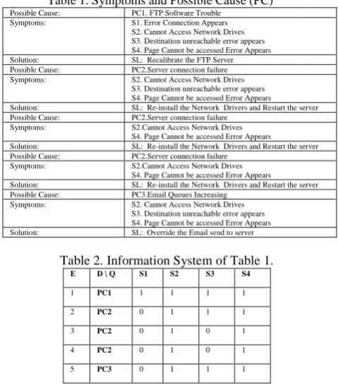
Table 1. Symptoms and Possible Cause (PC)

Possible Cause: PC1. FTP Software Trouble

Symptoms: S1. Error Connection Appears

S2. Cannot Access Network Drives S3. Destination unreachable error appears S4. Page Cannot be accessed Error Appears

Solution: SL: Recalibrate the FTP Server

Possible Cause: PC2.Server connection failure

Symptoms: S2. Cannot Access Network Drives

S3. Destination unreachable error appears S4. Page Cannot be accessed Error Appears

Solution: SL: Re-install the Network Drivers and Restart the server

Symptoms: S2.Cannot Access Network Drives

S4. Page Cannot be accessed Error Appears

Symptoms: S2.Cannot Access Network Drives

S4. Page Cannot be accessed Error Appears

Possible Cause: PC3.Email Queues Increasing

Symptoms: S2. Cannot Access Network Drives

S3. Destination unreachable error appears S4. Page Cannot be accessed Error Appears

Solution: SL: Override the Email send to server

Table 2. Information System of Table 1. E D \ Q S1 S2 S3 S4

1 PC1 1 1 1 1

2 PC2 0 1 1 1

3 PC2 0 1 0 1

4 PC2 0 1 0 1

5 PC3 0 1 1 1

Table 2 shows the Data in Table 1 converted to an Information System.

(3)

III. T

HEOREM

B

ASED ON

T

HE

R

OUGH

S

ET

T

HEORY

A. List of Mathematical Symbols

This research proposes a Theorem based on the Rough Set Theory about the Information Dependency of Data. It can be used in Incomplete Information Systems to find the correct Possible Cause. The following are the list of Mathematical Symbols used in this research and their explanations:

Table 3. List of Mathematical Symbols Symbol Name Explanation

IS Information System A 4–tuple_IS _ _D_,_Q_,_V_,_

D Set of Possible Causes It is a set of Possible Causes. For example PC1

- FTP Software Trouble, PC2 - Server connection failure and PC3 - Email Queues Increasing as shown in Table 2.2: D = {PC1, PC2, PC3}.

Q Set of Symptoms It is a set of Symptoms. For example S1 - Error

Connection Appears, S2 - Cannot Access Network Drives, S3 - Destination unreachable error appears and S4 - Page Cannot be accessed Error Appears as shown in Table 2.2

Q = {S1, S2, S3, S4}.

E Set of Cases E= {1,2,3,….a} for some natural numbera.

For example in Table 2.2 E = {1,2,3,4}.

V _{Codomain of}



For example in Table 2.2:

V = {1,0}.

 Relation fromDQ

to V

Letbe the relation from D  Q to V

which assigns at least one value for

) ( ) ,

(i j  EQ . For example in Table

2.2:

) 3 , 2 (PC S

 = 0 or 1

) 1 , 1 (PC S

 = 1

ab Index Indicates the location of a variable in a

Mathematical object. For example Mab, ab is

its index.

p Selected Possible cause It is the Possible cause selected from D in the

Information System. For example D = {PC1, PC2, PC3}. If PC1 is selected p = PC1.

p’ Other Possible causes Possible causes other than the selected Possible

cause p, that isp’is an element of D in the

Information System such thatp ' p .

q Selected Symptom It is the symptom selected from Q in the

Information System. For example Q = {S1, S2, S3, S4}. If S1 is selected it will be the q.

(p)(q)= f Notation Value or values associated with Selected Possible cause p and Selected Symptom q. Let

f be called the value of a

Symptom f  V .

For example in Table 2.2:

(PC1)(S1)={1} (PC2)(S3)={1,0} (PC3)(S1)={0}

* Unknown value The value is unknown

f

q Equality in associated_format. This is another way to write equality.qf

means q has a value of f. For example q = 1. It

can be written asq1.

=> IF THEN / Dependence

Notation q  f  D  p

means that if

(q=f) then the Possible Cause is p.

For example in (S1 = 1) => (D=PC1). If the value of the Selected Symptom S1 is 1 then it can be concluded that the Possible Cause is PC1

B. Theorem

Theorem 1: Consider an Information System

IS



D

,

Q

,

V

,



. Let p be a selected Possible Cause, q be a selected Symptom and let f be the value of selected Symptom. Assume

(

y

)(

q

)



*

for all

y



D

. If

(

p

)(

q

)

is a singleton,



and



(

p

'

)(

q

)

then



q



f

 



D



p



Observe that in the above theorem an Information System may be incomplete. However, the condition

*

)

)(

(

y

q



for all

y



D

requires that column q of the Information System be complete.

Proof:

Consider the sample Information System: Table 4. Information System of Data

E D \ Q Q1 Q2 Q3 Q4 …Qb

1 D1 C11 C12 C13 C14 …Cab

2 D2 C21 C22 C23 C24 …Cab

3 D3 C31 C32 C33 C34 …Cab

4 D4 C41 C42 C43 C44 …Cab

a Da Cab Cab Cab Cab Cab

In this example Information System Q Q Q Q Q b

Q  1, 2, 3, 4,...

D D D D D a

D  1, 2, 3, 4,...

 a

E  1,2,3,4...

C C C C C ab 

V  11 , 12 , 13 , 14 ...

Attributes Q1to Qbare Symptoms and D are the Possible causes.

q = Q1

p =D1

p’=D2, D3,D4,…Da

f = {C11}

11 1 C f Q q 

In the Information System

(

p

)(

q

)

is a singleton,



and



(

p

'

)(

q

)

The Information System will then be translated from tabular form to a logical form:

                                                                     a ab b ab ab ab ab ab b ab b ab b ab b D D C Q C Q C Q C Q C Q D D C Q C Q C Q C Q C Q D D C Q C Q C Q C Q C Q D D C Q C Q C Q C Q C Q D D C Q C Q C Q C Q C Q ( ) ( )... ( ) ( ) ( ) ( ) ( ) ( )... ( ) ( ) ( ) ( ) ( ) ( )... ( ) ( ) ( ) ( ) ( ) ( )... ( ) ( ) ( ) ( ) ( ) ( )... ( ) ( ) ( ) ( 4 3 2 1 4 44 4 43 3 42 2 41 1 3 34 4 33 3 32 2 31 1 2 24 4 23 3 22 2 21 1 1 14 4 13 3 12 2 11 1

Rewriting the equation in a simplified format:

) ... ( ) ... ( ) ... ( ) ... ( ) ... ( 4 3 2 1 4 3 2 1 4 3 2 1 4 3 2 1 4 3 2 1 4 44 43 42 41 3 34 33 32 31 2 24 23 22 21 1 14 13 12 11 a ab ab ab ab ab ab ab ab ab D C b C C C C D C b C C C C D C b C C C C D C b C C C C D C b C C C C D Q Q Q Q Q D Q Q Q Q Q D Q Q Q Q Q D Q Q Q Q Q D Q Q Q Q Q    

Writing the Decision Matrix for D1 Table 5. Decision Matrix

E 2 3 4 …a

1 Cab

b C

Q Q ...11

1 ab C b C Q Q11...

1 ab C b C Q Q 11...

1

a Cab

b C

Q Q ...11

1 Cab

b C

Q Q ...11

1 ab C b C Q Q 11...

(4)

Since the

q

f will always be present in all the intersections of the decision matrix in p then we can conclude that



q f

 

 Dp



.

An example when a system does not satisfy the conditions:

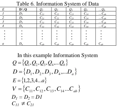
Consider the sample Information System: Table 6. Information System of Data

E D \ Q Q1 Q2 Q3 Q4 …Qb

1 D1 C11 C12 C13 C14 …Cab

2 D2 C21 C22 C23 C24 …Cab

3 D3 C31 C32 C33 C34 …Cab

4 D4 C41 C42 C43 C44 …Cab

a Da Cab Cab Cab Cab Cab

In this example Information System



Q Q Q Q Qb



Q ₁, ₂, ₃, ₄,...



D D D D Da



D 1, 2, 3, 4,...



a



E 1,2,3,4...



C C C C Cab



V  11, 12, 13, 14...

D1= D2= D1

C11



C21

Attributes Q1to Qbare Symptoms and D are the Possible causes.

q = Q1

p =D1

p’=D2, D3,D4,…Da

f = {C11,C21} 11, 21

1 C C f Q q 

In the Information System

(

p

)(

q

)

is not a singleton. The Information System will then be translated from tabular form to a logical form:

                                                                     a ab b ab ab ab ab ab b ab b ab b ab b D D C Q C Q C Q C Q C Q D D C Q C Q C Q C Q C Q D D C Q C Q C Q C Q C Q D D C Q C Q C Q C Q C Q D D C Q C Q C Q C Q C Q ( ) ( )... ( ) ( ) ( ) ( ) ( ) ( )... ( ) ( ) ( ) ( ) ( ) ( )... ( ) ( ) ( ) ( ) ( ) ( )... ( ) ( ) ( ) ( ) ( ) ( )... ( ) ( ) ( ) ( 4 3 2 1 4 44 4 43 3 42 2 41 1 3 34 4 33 3 32 2 31 1 2 24 4 23 3 22 2 21 1 1 14 4 13 3 12 2 11 1

Rewriting the equation in a simplified format:

) ... ( ) ... ( ) ... ( ) ... ( ) ... ( 4 3 2 1 4 3 2 1 4 3 2 1 4 3 2 1 4 3 2 1 4 44 43 42 41 3 34 33 32 31 2 24 23 22 21 1 14 13 12 11 a ab ab ab ab ab ab ab ab ab D C b C C C C D C b C C C C D C b C C C C D C b C C C C D C b C C C C D Q Q Q Q Q D Q Q Q Q Q D Q Q Q Q Q D Q Q Q Q Q D Q Q Q Q Q    

Writing the Decision Matrix for the Selected Possible Cause p which is D1

Table 7. Decision Matrix

1 ab C b C Q Q ...11

1 ab C b C Q Q 11...

1 2 ab C b C

Q

Q ...

21

1 ab C b C

Q

Q ...

21

1 ab C b C Q Q 21...

1

a

ab

C b

Q Cab

b

Q Cab

b Q

Since the

q

f will not be present in any of the intersections of the decision matrix in p then we can conclude that the equation



q



f

 



D



p



will not apply.

IV. DATA AND RESULTS

A. Presentation of Data on Computer Networks The Rough Based Decision Model and Theorem will be tested and validated using actual sample Data. The Data is represented into 2 categories, Possible Cause (PC) and Symptoms. The Data are the problems encountered by a Network Support Division or of a telecommunications company. These are the cases encountered in a Possible Cause and Symptom format. For Confidentiality purposes, the actual name of the company will not be disclosed.

Table 8. List of Symptoms and Possible Cause Possible Cause: PC1: OS Performs Illegal

Operations

Symptoms: S1: Conflict with TSR Running Program

S2: Computer Virus Message S7: Network Connection Error Appears

S9: MOM Alerts on Server: SVREBPPDBS01

Possible Cause: PC1: OS Performs Illegal Operations

Symptoms: S5: USB Virus message S8: Mapped Drive Cannot be accessed

Possible Cause: PC1: OS Performs Illegal Operations

S2: Computer Virus Message S3: Memory Overflow message appears

Possible Cause: PC2: LCA Cannot Be Accessed Symptoms: S1: Conflict with TSR Running

Program

S4: Error message regarding autoexec.bat or

S8: Mapped Drive Cannot be accessed

Possible Cause: PC2: LCA Cannot Be Accessed Symptoms: S2: Computer Virus Message

S6: The URL Cannot be accessed through the MDB

S10: MOM Alerts on Server: SVREBPPEBS32

Possible Cause: PC2: LCA Cannot Be Accessed Symptoms: S1: Conflict with TSR Running

(5)

Possible Cause: PC2: LCA Cannot Be Accessed Symptoms: S3: Memory Overflow message

appears

Possible Cause: PC3: Kronos problem Symptoms: S2: Computer Virus Message

S7: Network Connection Error Appears

S12: SVRMDBADDC12 Cannot be accessed

Possible Cause: PC3: Kronos problem

S3: Memory Overflow message appears

Possible Cause: PC3: Kronos problem

Possible Cause: PC3: Kronos problem Symptoms: S5: USB Virus message

Possible Cause: PC4: Network IP Address Conflict Symptoms: S2: Computer Virus Message

S11: SVR-MDBSPPS-01 Cannot be accessed

Possible Cause: PC4: Network IP Address Conflict Symptoms: S8: Mapped Drive Cannot be

accessed

Possible Cause: PC4: Network IP Address Conflict Symptoms: S2: Computer Virus Message

S11: SVR-MDBSPPS-01 Cannot

be accessed

Possible Cause: PC4: Network IP Address Conflict Symptoms: S1: Conflict with TSR Running

Program

Possible Cause: PC5: CPU COM/Serial Port Problem

Symptoms: S3: Memory Overflow message appears

S2: Computer Virus Message Possible Cause: PC6: OS Disk Error

Symptoms: S3: Memory Overflow message appears

Possible Cause: PC6: OS Disk Error Symptoms: S4: Error message regarding

autoexec.bat or

S5: USB Virus message Possible Cause: PC6: OS Disk Error

Symptoms: S2: Computer Virus Message S3: Memory Overflow message appears

Possible Cause: PC7: FTP Server Trouble Symptoms: S3: Memory Overflow message

appears

Possible Cause: PC7: FTP Server Trouble Symptoms: S1: Conflict with TSR Running

Program

(6)

be accessed

Possible Cause: PC8: Internet Email cannot received/sent

S5: USB Virus message S9: MOM Alerts on Server: SVREBPPDBS01

Possible Cause: PC9: Network Adapter Error Symptoms: S1: Conflict with TSR Running

Program

S2: Computer Virus Message Possible Cause: PC9: Network Adapter Error Symptoms: S1: Conflict with TSR Running

Program

Possible Cause: PC9: Network Adapter Error Symptoms: S3: Memory Overflow message

appears

S9: MOM Alerts on Server:

SVREBPPDBS01

Program

S5: USB Virus message S10: MOM Alerts on Server: SVREBPPEBS32

Program

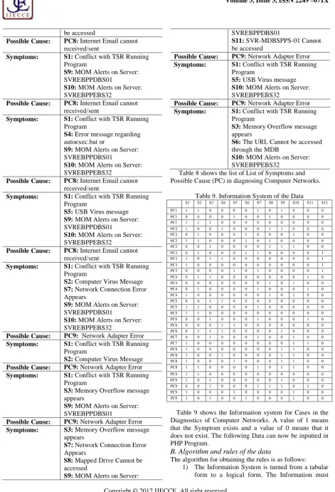
Table 8 shows the list of List of Symptoms and Possible Cause (PC) in diagnosing Computer Networks.

Table 9. Information System of the Data

S1 S2 S3 S4 S5 S6 S7 S8 S9 S10 S11 S12

PC1 1 1 0 0 0 0 1 0 1 0 0 0

PC1 0 0 0 0 1 0 0 1 0 0 0 0

PC1 1 1 1 0 0 0 0 0 0 0 0 0

PC2 1 0 0 1 0 0 0 1 1 0 0 0

PC2 0 1 0 0 0 1 0 0 0 1 0 0

PC2 1 1 0 0 0 1 0 1 0 0 0 0

PC2 0 0 1 0 0 0 0 1 1 1 0 0

PC3 0 1 0 0 0 1 1 0 0 0 0 1

PC3 1 0 1 1 0 0 0 0 0 0 0 1

PC3 1 0 0 0 0 0 0 0 0 0 0 1

PC3 0 0 0 0 1 0 1 0 0 0 0 1

PC4 0 1 1 0 0 0 0 0 0 0 1 0

PC4 0 0 0 0 0 0 0 1 0 1 0 0

PC4 0 1 0 0 0 0 1 0 0 0 1 0

PC4 1 0 0 0 0 0 0 1 0 1 0 0

PC5 0 0 1 1 0 0 0 0 0 0 0 0

PC5 1 1 0 0 0 0 1 0 0 0 0 0

PC5 1 1 0 0 0 0 0 0 0 0 0 0

PC6 0 0 1 0 0 0 1 0 0 0 1 0

PC6 0 0 0 1 1 0 0 0 0 0 0 0

PC6 0 1 1 1 0 0 0 0 1 0 0 0

PC7 0 0 1 0 0 0 1 0 0 1 0 0

PC7 1 0 0 0 0 0 0 0 0 1 1 0

PC8 1 0 0 0 0 0 0 0 1 1 0 0

PC8 1 0 0 1 0 0 0 0 1 1 0 0

PC8 1 0 0 0 1 0 0 0 1 1 0 0

PC8 1 1 0 0 0 0 1 0 1 1 0 0

PC9 1 1 0 0 0 0 0 0 0 0 0 0

PC9 1 0 1 0 0 0 0 0 1 0 0 0

PC9 0 0 1 0 0 0 1 1 1 0 1 0

PC9 1 0 0 0 1 0 0 0 0 1 0 0

PC9 1 0 1 0 0 1 0 0 0 1 0 0

Table 9 shows the Information system for Cases in the Diagnostics of Computer Networks. A value of 1 means that the Symptom exists and a value of 0 means that it does not exist. The following Data can now be inputted in PHP Program.

B. Algorithm and rules of the data

The algorithm for obtaining the rules is as follows: 1) The Information System is turned from a tabular

(7)

(DNF) of propositional logic.

2) The equalities are written in associated format. 3) The Information is written as a Decision Matrix

for each Possible Cause (PC). The rows will contain the values where the symptoms are present and the columns will contain the symptoms that are not present. In the intersections of the Decision Matrix, write the symptoms of the Target Possible Cause and where the symptoms are equal to in associated format.

4) Each Decision Matrix will form a set of Boolean Expressions. There will be one expression for each row of the matrix. The items that are in each cell are disjunctively accumulated. The individual cells are also conjunctively accumulated.

5) The output parameters will be simplified using Boolean algebra.

6) Repeat the process for each Possible Cause. 7) Write the simplified output parameters as an

Information System.

8) Each Row in the Information System will be written as a Rule in the form of:



q



f

 



D



p



. If there are two or more dependent Symptoms they are Conjunctively

Accumulated. The Symptoms with a “*” value

will not be considered. 9) Remove Redundant Rules

10) Possible Cause with the same set of conditions will be written as Approximate Rules

The rules are then produced using the PHP Program which applied the algorithm. The PHP Program uses the ROSE (Rough Set Data Explorer) libraries [13]. ROSE was developed at the Laboratory of Intelligent Decision Support Systems of the Institute of Computing Science in Poznan [14]. The rules were generated in our system with one approximate rule, the rules are:

Table 10. Rules of the Data

Rule 1 (S7 = 1) & (S8 = 0) & (S9 = 1) & (S10 = 0) => (PC = 1)

Rule 2 (S4 = 0) & (S5 = 1) & (S10 = 0) & (S12 = 0) => (PC = 1)

Rule 3 (S1 = 1) & (S2 = 1) & (S3 = 1) => (PC = 1) Rule 4 (S4 = 1) & (S8 = 1) => (PC = 2) Rule 5 (S2 = 1) & (S6 = 1) & (S12 = 0) => (PC = 2) Rule 6 (S3 = 1) & (S9 = 1) & (S10 = 1) => (PC = 2)

Rule 7 (S12 = 1) => (PC = 3)

Rule 8 (S2 = 1) & (S11 = 1) => (PC = 4)

Rule 9 (S2 = 0) & (S3 = 0) & (S4 = 0) & (S5 = 0) & (S8 = 1) => (PC = 4)

Rule 10 (S4 = 1) & (S5 = 0) & (S9 = 0) & (S12 = 0) => (PC = 5)

Rule 11 (S1 = 1) & (S7 = 1) & (S9 = 0) => (PC = 5) Rule 12 (S4 = 1) & (S5 = 1) => (PC = 6)

Rule 13 (S3 = 1) & (S7 = 1) & (S8 = 0) & (S11 = 1) => (PC = 6)

Rule 14 (S3 = 1) & (S4 = 1) & (S9 = 1) => (PC = 6)

Rule 15 (S5 = 0) & (S6 = 0) & (S8 = 0) & (S9 = 0) & (S10 = 1) => (PC = 7)

Rule 16 (S1 = 1) & (S9 = 1) & (S10 = 1) => (PC = 8) Rule 17 (S3 = 1) & (S4 = 0) & (S9 = 1) & (S10 = 0) => (PC = 9)

Rule 18 (S2 = 0) & (S7 = 0) & (S8 = 0) & (S9 = 0) & (S10 = 1) & (S11 = 0) => (PC = 9)

Approximate Rules

Rule 19 (S2 = 1) & (S3 = 0) & (S7 = 0) & (S8 = 0) & (S10 = 0) => (PC = 5) OR (PC = 9)

In Table 10 the IF THEN Rules means that if that if this Set of Symptoms exist or does not exist then this is the Possible Cause. A value of 1 means the symptom exist and a value of 0 means it does not exist. For example in Rule 5 where (S2 = 1) & (S6 = 1) & (S12 = 0) => (PC = 2). It means that if S2 (Computer Virus Message), S3 (Memory Overflow message appears) exist and S12 (SVRMDBADDC12 Cannot be accessed) does not exist then the Possible Cause is PC2 (LCA Cannot Be Accessed).

C. Empirical Testing

The first part of the Validation process is Empirical Testing. The Validating Data will be composed of the technical data. An Example for the process is in Rule 16 (S1 = 1) & (S9 = 1) & (S10 = 1) => (PC = 8), meaning if S1 (Conflict with TSR Running Program), S9 (MOM Alerts on Server: SVREBPPDBS01 and S10 (MOM Alerts on Server: SVREBPPEBS32) exist the problem is PC8 (Internet Email cannot received/sent). The initial Information System will be checked if S1, S9 and S10 exist in a case in PC8. The cases in the Information System were tested on generated rules and all gave the correct values.

The following are the detailed steps on how to perform this validation process.

a. Prepare the validating data

The validating data will be composed of the technical data where the rules are created.

b. Check each rule with the validating data to see if the values matched.

Example in Rule 16: PC = 8 if S1 = 1, S9 = 1 and S10 = 1. Check if there is a case in PC8 where S1 = 1, S9 = 1 and S10 = 1.

Table 11. Checking of Rule 16

c. Repeat the process for each rule and record how many rules satisfied the condition.

Table 12. Empirical Test on the Rules

Case Value of Symptoms in Cases

Rule 1 (S7 = 1) & (S8 = 0) & (S9 = 1) & (S10 = 0) => (PC = 1)

PC1 S7 = 1, S8 = 0, S9 = 1, S10 = 0

Rule 2 (S4 = 0) & (S5 = 1) & (S10 = 0) &

(S12 = 0) => (PC = 1)

PC1 S4 = 0, S5 = 1, S10 = 0, S12 = 0

Rule 3 (S1 = 1) & (S2 = 1) & (S3 = 1) =>

(PC = 1)

PC1 S1 = 1, S2 = 1, S3 = 1

Rule 4 (S4 = 1) & (S8 = 1) => (PC = 2) PC2 S4 = 1, S8 = 1

Rule 5 (S2 = 1) & (S6 = 1) & (S12 = 0) =>

(PC = 2)

PC2 S2 = 1, S6 = 1, S12 = 0

Rule 6 (S3 = 1) & (S9 = 1) & (S10 = 1) =>

(PC = 2)

PC2 S3 = 1, S9 = 1, S10 = 1

Rule 7 (S12 = 1) => (PC = 3) PC3 S12 = 1

Rule 8 (S2 = 1) & (S11 = 1) => (PC = 4)

(8)

Table 12 showed the Empirical Test on the rules. All the rules satisfied the possible cause when compared with the data and proved the validity of the rules.

The Theorem is also evident PC3 (Kronos problem). It satisfied the conditions on the theorem therefore it is Information dependent on the value if S12 (SVRMDBADDC12 Cannot be accessed) existing or having a value 1.

D. Test with previous Live Data

The rules that are created will be checked with previous live data. It will be used as the Validating data. These data are obtained through retrieval of the information in a live scenario and the Possible Cause is known. It will be checked with the Rules that are created using the Rough Set Decision Model.

a. Enter Previous live Data

b. Check if the Possible Cause outputted of the Expert System equals to the Possible Cause of the Validating DataExample in Case 4 which has S3 (Memory Overflow message appears), S8 (Mapped Drive Cannot be accessed), S9 (MOM Alerts on Server: SVREBPPDBS01) and S10 (MOM Alerts on Server: SVREBPPEBS32) as the symptoms, the expected output is PC2 (LCA Cannot Be Accessed). When inputted in the system it gave PC2 as the output same as the expected.

c. Repeat the process for each validating Data. The number of Possible Cause that are outputted correctly out of the total previous live cases will be the score for this test.

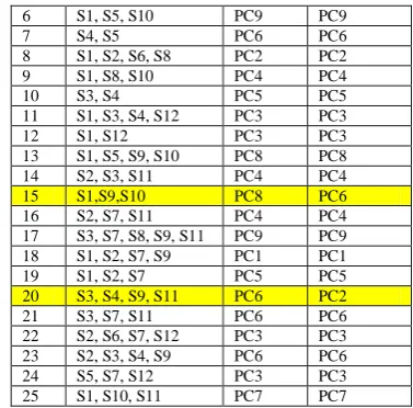
Table 13. Test with previous live data

Case Symptoms System

Output

Expected Output

1 S1, S2, S7, S9, S10 PC8 PC8

2 S5, S8 PC1 PC1

3 S3, S7, S10 PC7 PC7

4 S3, S8, S9, S10 PC2 PC2

5 S1, S2, S3 PC1 PC1

6 S1, S5, S10 PC9 PC9

7 S4, S5 PC6 PC6

8 S1, S2, S6, S8 PC2 PC2

9 S1, S8, S10 PC4 PC4

10 S3, S4 PC5 PC5

11 S1, S3, S4, S12 PC3 PC3

12 S1, S12 PC3 PC3

13 S1, S5, S9, S10 PC8 PC8

14 S2, S3, S11 PC4 PC4

15 S1,S9,S10 PC8 PC6

16 S2, S7, S11 PC4 PC4

17 S3, S7, S8, S9, S11 PC9 PC9

18 S1, S2, S7, S9 PC1 PC1

19 S1, S2, S7 PC5 PC5

20 S3, S4, S9, S11 PC6 PC2

21 S3, S7, S11 PC6 PC6

22 S2, S6, S7, S12 PC3 PC3

23 S2, S3, S4, S9 PC6 PC6

24 S5, S7, S12 PC3 PC3

25 S1, S10, S11 PC7 PC7

Table 13 shows the test done when tested with previous live data. The one’s highlighted are where the System’s

Output is not equal to the Expected Output. All the output of the cases was given by the system. This test gave 23 / 25 or a 92% result and showed the Rough Set Based

Decision Model’s competence in previous live data.

V. A

NALYSIS AND

C

ONCLUSION

This research showed a Rough Set Based Decision model that can be used in the diagnostics of Computer Networks. This research used the Rough Set Theory in Computer Networks to convert its technical data into the nominal rules meaning only the necessary information needs to be inputted to find the Possible Cause. In cases where the Data gathered is incomplete, the proper conclusion may still be suggested. The created rules are tested to verify its validity.

A theorem based on the Rough Set Theory is also proposed on the Information Dependency of data, the essential information needed in order to find the Possible Cause. A formal proof of the theorem was presented and its correctness was tested on live data. It is very vital and useful in large Information Systems. Knowing which Data is needed will not only save time in the processing of information but also conserve resources.

The Decision Model and Theorem in this research can be applied in Artificial Intelligence Based Systems like Expert Systems. A future recommendation for this research is for it to be tested in other fields. The scope of this research is only for Information System Communication Networks. In theory, the theorem and algorithm can be applied in several Production Systems with a Possible Cause and Symptom relationship.

R

EFERENCES

[1] T. Beaubouef and R. Lang, “Rough set techiques for uncertainty management in automated story generation”. Proceedings of the

36th annual Southeast regional conference. pp 326-331, 1996

Rule 9 (S2 = 0) & (S3 = 0) & (S4 = 0) &

(S5 = 0) & (S8 = 1) => (PC = 4)

PC4 S2 = 0, S3 = 0, S4 = 0,

S5 = 0, S8 = 1

Rule 10 (S4 = 1) & (S5 = 0) & (S9 = 0) &

(S12 = 0) => (PC = 5)

PC5 S4 = 1, S5 = 0, S9 = 0,

S12 = 0

Rule 11 (S1 = 1) & (S7 = 1) & (S9 = 0) =>

(PC = 5)

PC5 S1 = 1, S7 = 1, S9 = 0

Rule 12 (S4 = 1) & (S5 = 1) => (PC = 6) PC6 S4 = 1, S5 = 1

Rule 13 (S3 = 1) & (S7 = 1) & (S8 = 0) &

(S11 = 1) => (PC = 6)

PC6 S3 = 1, S7 = 1, S8 = 0, S11 = 1

Rule 14 (S3 = 1) & (S4 = 1) & (S9 = 1) =>

(PC = 6)

PC6 S3 = 1, S4 = 1, S9 = 1

Rule 15 (S5 = 0) & (S6 = 0) & (S8 = 0) & (S9 = 0) & (S10 = 1) => (PC = 7)

PC7 S5 = 0, S6 = 0, S8 = 0,

S9 = 0, S10 = 1

Rule 16 (S1 = 1) & (S9 = 1) & (S10 = 1) => (PC = 8)

PC8 S1 = 1, S9 = 1, S10 = 1

Rule 17 (S3 = 1) & (S4 = 0) & (S9 = 1) & (S10 = 0) => (PC = 9)

PC9 S3 = 1, S4 = 0, S9 = 1,

S10 = 0

Rule 18 (S2 = 0) & (S7 = 0) & (S8 = 0) & (S9 = 0) & (S10 = 1) & (S11 = 0) => (PC = 9)

PC9 S2 = 0, S7 = 0, S8 = 0,

S9 = 0, S10 = 1, S11 = 0

Approximate Rules Rule 19 (S2 = 1) & (S3 = 0) & (S7 = 0)

& (S8 = 0) & (S10 = 0) => (PC = 5) OR (PC = 9)

PC9 OR PC5

(9)

consumers using rough sets”, Digital Object Identifier. Vol 4, No, 2004.

[3] A. Diaz, J. Wang, L. Quintero, C. Coello, R. Caballero and J.

Molina. “A New Proposal for Multi-Objective Optimization

using Differential Evolution and Rough Sets”. Proceedings of the 8th annual conference on Genetic and evolutionary computation. pp 675-682. 2006.

[4] Z. Palwak. “Rough Sets”. International Journal of Information in

Computer Science. Vol 11, No 5, 1982.

[5] J. Liang, J. Wang and Y. Qian. “A new measureof uncertainty

based on knowledge granulation for rough sets”. Information

Sciences. Vol 179, No 4, pp 458-470, 2009.

[6] L. Zhou, W. Wu and W. Zhang. “On characterization of

intuitionistic fuzzy rough sets based on intuitionistic fuzzy

implicators”. Information Sciences. Vol 179, No 7, pp 883-898, 2009.

[7] A. Africa and C. Co. “Development of a Rough Set Based Model in Computere Diagnostics”. 13th International Conference on

Mechatronics Technology–ICMT. 2009

[8] Z. Palwak. “Rough Sets: Theoretical Aspects of Reasoning about

Data”. Boston, MA: Kluwer, 1991.

[9] W. Ziarko and S. Regina. “A brief introduction to Rough Sets”.

The First International Workshop on Rough Sets: State of the art perspective. Vol 14, No 3, pp. 29-31, 1993.

[10] N. Shan, W. Ziarko, H. Hamilton and N. Cercone.” Using

Rough Sets as Tools for Knowledge Discovery from Large

Relational Databases”. 1st conference on knowledge discovery

and Data Mining. pp 263-268, 1995.

[11] W. Ziarko. “Discovery through Rough Set”. Communications of the ACM. Vol 42, No 11, 1999.

[12] A. Pauly and M. Schneider. “ROSA: An Algebra for Rough Spatial Objects in Databases”. Proceedings of the 2008 ACM

symposium on Applied computing. 875-879, 2009 [13] ROSE 2.0 http://www.-idss.cs.put.poznan.pl/rose. 1999 [14] P. Bartolomiej, R. Slowinsky, J. Stefanowsky, R. Susmaga and

S. Wilk. “ROSE- Software Implementation of the Rough Set

Theory.” Lecture Notes in Computer Science. Vol 1242, No 2,

pp 605-608.

A

UTHOR

’

S

P

ROFILE

Aaron Don M. Africa