R E V I E W
Open Access
Nonlinear dynamical analysis of
GNSS data: quantification, precursors
and synchronisation
Bruce Hobbs
1,3*and Alison Ord
1,2Abstract
The goal of any nonlinear dynamical analysis of a data series is to extract features of the dynamics of the underlying physical and chemical processes that produce that spatial pattern or time series; a by-product is to characterise the signal in terms of quantitative measures. In this paper, we briefly review the methodology involved in nonlinear analysis and explore time series for GNSS crustal displacements with a view to constraining the dynamics of the underlying tectonic processes responsible for the kinematics. We use recurrence plots and their quantification to extract the invariant measures of the tectonic system including the embedding dimension, the maximum Lyapunov exponent and the entropy and characterise the system using recurrence quantification analysis (RQA). These measures are used to develop a data model for some GNSS data sets in New Zealand. The resulting dynamical model is tested using nonlinear prediction algorithms. The behaviours of some RQA measures are shown to act as precursors to major jumps in crustal displacement rate. We explore synchronisation using cross- and joint-recurrence analyses between stations and show that generalised synchronisation occurs between GNSS time series separated by up to 600 km. Synchronisation between stations begins up to 250 to 400 days before a large displacement event and decreases immediately before the event. The results are used to speculate on the coupled processes that may be responsible for the tectonics of the observed crustal deformations and that are compatible with the results of nonlinear analysis. The overall aim is to place constraints on the nature of the global attractor that describes plate motions on the Earth.
Keywords:GNSS time series, Nonlinear analysis, Dynamical systems, Recurrence plots, Recurrence quantification analysis (RQA), Cross and joint recurrence plots, Crustal deformation, Precursors, Synchronisation
Introduction
The general nature of the dynamics of the mantle of the Earth along with the interaction of the mantle with the lithosphere is thought to be well known; broadly, con-vective motion in the mantle with coupled thermal and mass transport results in tractions on the bases of the lithospheric plates. These tractions together with other tractions generated by instabilities, such as subducting slabs along with forces generated by spreading from mid-ocean ridges, lead to plate motions expressed as plate deformations observed at the surface of the Earth in the form of GNSS (Global Navigation Satellite
System) measurements. Fundamental questions are do the displacements we observe synchronise in some way from one place to another? And if so, on what spatial and time scales does synchronisation occur? Can the pat-tern of synchronisation be used to define precursors to major and commonly destructive displacement events? The global array of GNSS measurements and their time series should, on principle, give enough information to construct the dynamics of the underlying processes and answer such questions. However, in order to be more specific, one needs to better express the partial differen-tial equations that describe the processes responsible for the dynamics and the ways in which these processes are coupled and evolve with time. With the present uncer-tainties regarding constitutive relations and properties and the temperature distribution within the Earth, it is difficult to constrain possible geometric and kinematic * Correspondence:[email protected]
1Centre for Exploration Targeting, School of Earth Sciences, University of
Western Australia, Perth, Western Australia 6009, Australia 3CSIRO, Perth, Western Australia 6102, Australia
Full list of author information is available at the end of the article
models for plate development and evolution with com-puter models based on current knowledge of these issues and with the available computing power. The results of any such models should at least be compatible with the results of detailed analysis of observed crustal displace-ment data which is the purpose of this paper.
The main data sets we have at present that are useful in developing such constraints are geophysical data sets (gravity, magnetics and seismic), heat flow measure-ments, the distribution of topography on the surface of the Earth and GNSS data on crustal displacements. These latter data sets are now well distributed over the Earth, and in some instances, continuous time series go back at least a decade. We concentrate on GNSS data in this paper with the aim of establishing how much of the dynamics of the plate tectonic processes is reflected in such data. Future papers attempt to integrate these data sets. Just as the global weather system is an expression of the Navier-Stokes equations for a viscous fluid with coupled heat and mass transport and which result in highly nonlinear behaviour, we expect the dynamics underlying plate tectonics to be highly nonlinear. The aim is to characterise and quantify this behaviour and, as far as is possible, move towards identifying the mathem-atical expression of the coupled processes that operate to produce crustal deformation driven by plate motions.
Nonlinear time series analysis and dynamical systems
The nature of nonlinear time series analysis
The aim of time series analysis is to classify and quantify the nature of a particular time series of interest and, if possible, understand the dynamics of the processes that operated to produce the time series. Most approaches to such a task in the geosciences consider linear stochastic models commonly with an assumed Gaussian or log-normal distribution for the data. This essentially means that one assumes the data to be stochastic, that is, the result of uncorrelated linear processes. The linear assumption implies that the law of superposition (Hobbs and Ord2015, pp. 10–15) is valid so that iff(x) andg(x) describe the dynamics of a system, then linear combina-tions of f(x) and g(x) also define the dynamics. Such an assumption implies that Fourier methods are useful in characterising the data (Stoica and Moss2005). The sto-chastic assumption assumes no long-range correlations in the data. Analysis is difficult if the data are non-stationary (the mean and/or the standard deviation vary with time), there is considerable noise in the data and “outliers” (departures from Gaussian or log-normal distributions) are common. Nevertheless, the data are often forced to fit stationary, Gaussian distributions with no long-range correlations and methods such as kriging, co-kriging, autoregressive and moving average methods
and power spectra together with filtering/smoothing procedures are employed. Such methods are parametric (a statistical distribution is assumed for the data) and have no conceptual link to the underlying processes that produced the data. The stationary stochastic Gaussian time series, consisting of the terms {x1, x2, ….., xN},
where N is the total number of terms, is commonly characterised using Fourier transform methods and by the autocorrelation function,c(τ):
cð Þ ¼τ ðxi−xiþτÞ
2
x2
i
ð1Þ
whereτis called thelagand the 〈∗〉brackets denote the
mean of the quantities involved (Box et al.2008). Noise
reduction is commonly thought of as a smoothing oper-ation, the premise being that smooth data are better in some unspecified way than irregular data, and is com-monly undertaken using recursive Bayesian procedures such as in the Kalman filter and its variants (Judd and
Stemler2009).
The outcome of any time or spatial series analysis is a
data modelwhich enables one to characterise the statis-tical measures (mean, standard deviation, autocorrel-ation function, power spectrum and so on) of the data and if possible undertake forecasts, interpolations and extrapolations of the data. We distinguish two classes of data models; one is a parametric stochastic data model that assumes an underlying statistical distribution and has no relation to the underlying processes that pro-duced the data. The other is a non-parametric determin-istic data model that makes no assumptions about the underlying statistics and directly reflects the dynamics of the system. The linear, stochastic procedures of kriging, co-kriging, autoregressive and moving average methods work well for linear systems where the law of superpos-ition holds and Fourier methods clearly delineate discrete periodicities in the data. These are methods of constructing a stochastic, parametric data model. How-ever, in nonlinear systems, especially those that are cha-otic, these methods fail; the assumptions of Gaussian or log-normal distributions with no long-range correlations break down. Nonlinear signal processing methods (Small 2005) become not only essential but are capable of de-lineating the nature of the processes that operated or of testing models of processes that might be proposed (Judd and Stemler 2009; Small 2005). We paraphrase Judd and Stemler (2010): Understanding: it is not about the statistics, it is about the dynamics.
quantity. Thus, for a sliding frictional surface where the only processes might be velocity-dependent frictional soft-ening, accompanied by heat production and chemical healing of damage, the behaviour is described in a four-dimensional state space with coordinates comprising the state variables, velocity, temperature, friction coeffi-cient and degree of chemical healing. A time series for temperature is a projection from the four-dimensional state space on to a one-dimensional time series. Quantities that appear close together in the time series may in fact be widely separated in state space. With respect to the GNSS time series from New Zealand that we examine in this paper, the deforming crustal system operates in a state space where at least the state variables velocity, stress, strain-rate, temperature, damage-rate, healing-rate and fluid pressure are needed to define the system; there prob-ably are others involving the ways in which one part of the system is coupled to other parts. The GNSS displacement signal we observe is the projection from a space defined by these state variables on to a single displacement record that we observe at a particular station as a one dimen-sional time series.
As opposed to stochastic data models based on Gauss-ian statistics, lack of long-range correlations and the principle of superposition, the nonlinear systems we are interested in studying in the geosciences result from clearly defined physical and chemical processes. Al-though we may have considerable trouble in discovering and characterising these processes, the system is deter-ministic rather than stochastic. Hence, in principle, we should be able to define for a system of interest the in-variant measures that characterise the system. An invari-ant measure remains the same independently of the way in which the system is observed and so remains the same independently of the dimensions of the state space in which we observe the system. Such measures include the Rényi generalised dimensions (including the fractal support dimension and the correlation dimension for the system) that characterise the geometry and are de-fined from a multifractal spectrum for the system (Beck and Schlögl1995; Arneodo et al.1995; Ord et al.,2016), theLyapunov exponentsthat are related to thedynamics
of the system and define the stability of the system and how far prediction is possible (Small2005) and the Kol-mogorov-Sinai entropy, related to information theory, that tells us how much information exists in the signal and is also related to predictability (Beck and Schlögl 1995; Small2005). We will estimate these invariant mea-sures for GNSS time series together with a number of other quantitative measures but not dwell too heavily on the mathematics behind the theory. Readers who require in-depth treatments should consult (Abarbanel 1996; Beck and Schlögl1995; Sprott2003; Kantz and Schreiber 2004; Small 2005; Judd and Stemler2010). This paper is
a brief review of nonlinear analysis with an emphasis on
recurrence methods (Marwan et al. 2007a). The princi-ples are illustrated using specific examprinci-ples from the Lo-rentz system (Sprott 2003, p. 205) and several GNSS time series from New Zealand.
The invariant measures
The basis of nonlinear analysis lies in powerful proposals put forward by Crutchfield (1979) and Packard et al. (1980) and proved rigorously by Takens (1981). What is commonly referred to asTakens’ theoremstates that the complete dynamics of a system can be derived from a time series for a single state variable from that system. The reason for this (as expressed in the friction example above) is that in systems where all the state variables are coupled, the behaviour of one depends on the behaviours of all the others and so the time series for one variable has the behaviours of all the other variables encoded within it. Thus, if we have a time series {x1, x2, ….., xN}, then we can construct M-dimensional reconstruction space vectors, M(t), from M time delayed samples so that the vector Mis:
Mð Þ ¼t ½x tð Þ;x tð þτÞ;x tð þ2τÞ; ::……;x tð þðM−1ÞτÞ ð2Þ
In this process, every point in the signal is compared with a point distant τ away. These vectors define the
attractorfor the system; this is the manifold that all pos-sible states of the system can occupy independently of the initial conditions. If in this construction, the delay,τ,
one can identify a dimension where the number of false neighbours is zero then one has a good estimate of the embedding dimension. For white noise, the percentage of false neighbours remains at 50% independent of the dimension of the space in which the signal is observed.
One can also identify another dimension that we call thedynamical orstate dimension, D. This is the dimen-sion, it may or may not be an integer, that is the true di-mension of the attractor. Generally, D is difficult to measure because of noise andDis attenuated because of non-stationary behaviour or local variability in attractor density of states so that D≥D. D can be estimated dir-ectly from the time series whereas Dcan only be mea-sured if we have access to a well-defined attractor (Packard et al.1980; Ord1994).
The embedding dimension can be estimated by plot-ting the number of false neighbours against the embed-ding dimension (this is done for the Lorentz attractor in Fig. 7c and for GNSS data in Fig. 13). This plot ideally has a minimum at the embedding dimension (Small 2005). In addition, if one defines the correlation dimen-sion,C2, for a time series with N data points:
C2ðD;εÞ ¼
1 2N Nð −TÞ
X
i
X
j<i−T
Θ ε−xi−xj
ð3Þ
whereΘ(*) is the Heaviside function, and T is a
param-eter large enough that it ensures the distances between points are distributed so that no biases exist towards
small numbers, thenC2(D,ε) represents the fraction, in
embedding space, of pairs of points separated by
Euclid-ian distances smaller thanε. A plot ofC2against
embed-ding dimension (see Fig. 7b) ideally has an initial slope
of 45° and reaches a plateau at the embedding dimen-sion. Details of methods of estimating the embedding
di-mension are spelt out by Small (2005) together with the
pitfalls involved.
Recurrence plots and recurrence quantification
Recurrence plots
Although nonlinear signal processing is at least 30 years old (Abarbanel 1996; Beck and Schlögl 1995; Sprott 2003; Kantz and Schreiber 2004; Small 2005; Judd and Stemler2010), most approaches are fairly opaque to po-tential users. Hence, particularly in the geosciences, the inertia involved in using such developments is very large. However, a step in overcoming the inertia was made by Eckmann et al. (1987) who introduced the concept of re-currence plots which are generalised autocorrelation functions based on Takens’ theorem and derived from the conclusion reached by Poincaré (1890) for nonlinear systems that….., neglecting some exceptional trajectories,
the occurrence of which is infinitely improbable, it can be shown, that the system recurs infinitely many times as
close as one wishes to its initial state. Since Eckmann’s
classical paper, the subject has expanded dramatically with important contributions from Casdagli (1997), Webber and Zbilut (2005) and Marwan et al. (2007a). The literature is now very large especially in climate studies, biology and medicine; applications to seismic studies are Chelidze and Matcharashvili (2015) and Gar-cia et al. (2013) but other applications in the geosciences are rare. Generalised recurrence plots forn-dimensional spatial data sets are discussed in Marwan et al. (2007b). If the dimensions of the system aren then the general-ised recurrence plot is in 2n-space. Thus, a recurrence plot for three-dimensional data exists in 6-space. We only consider one-dimensional data sets in this paper.
A recurrence plot is a symmetrical matrix, Rij,
expressed as a two-dimensional visualisation and defined by
Rij¼Θ ε−xi−xj
for i;j¼1;N ð4Þ
where ε is an arbitrary threshold distance (commonly
called the radius) that measures the tolerance within
which recurrence is identified and ‖∗‖ denotes a norm,
commonly taken as the Euclidean norm. (4) says that we
measure the distance between a given point, xi, on the
signal and every other point,j= 1 to N on the signal and
give that measure the value 1 if the distance is within
the tolerance, ε, or zero if not. This is repeated for all
values of i= 1 to N to form the recurrence matrix. The
caveat is that the distances are measured in the
embed-ding space. A recurrence plot is then a plot of Rij for a
given radius, ε. If ‖xi−xj‖≈ε then Rij= 1 and a dot is
added to the plot; otherwise, Rij= 0 and the plot are left
blank. The plot may be contoured by setting ‖xi−xj‖≈
0.8ε, 0.6ε, ...0.2εand so on. In some software (VRA), the
contour interval is prescribed within the software; for
others, a number,c, can be set which defines the number
of contours with equal spacing, (ε /c). We repeat, a
preserved (Fig. 1c). Recurrence plots are applicable to stationary and nonstationary data sets and are reason-ably insensitive to noise. Pitfalls associated with recur-rence analysis are discussed by Marwan (2011).
Recurrence quantification
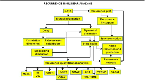
Although recurrence plots make “pretty pictures” (espe-cially ifεis large andcis small) and are useful for com-paring and visually classifying different data sets, the real power lies in the quantitative measures, including the in-variant measures, that can be derived from them. In principle, because of Takens’theorem, all of the dynam-ics of the system are encoded in the recurrence plot and the quantitative measures are designed to expose the dy-namics. Recurrence quantification analysis (RQA) is based on deriving quantitative information from the dis-tribution of lines on the recurrence plot. For a detailed discussion of these measures, see Webber and Zbilut (2005) and Marwan et al. (2007a); in Table1, we present a summary of many of these measures. Figure2shows a summary of many of the steps involved in, and outputs
from, an RQA and we will elaborate upon this diagram later in the paper with respect to GNSS data sets.
The recurrence plots shown in Fig. 1 are relatively simple and represent completely stochastic systems (Fig. 1a) or completely deterministic systems (Fig. 1b). Most natural systems lie somewhere between these two extremes. An example is given in Fig.3which is the re-currence plot for one of the time series from the Lorentz system (Sprott 2003) examined in greater detail later in the paper. The recurrence plot, which here has been constructed to emphasise the main features in typical re-currence plots, consists of many vertical and horizontal lines as well as diagonal lines. Below, we consider the significance of these lines; they are the basis for RQA.
Note that two invariant measures may be derived from the recurrence plot. The entropy is given by ENT: for periodic signals, ENT = 0 bits/bin, and for the Hénon attractor (Sprott 2003, p. 421), ENT = 2.557 bits/bin (Webber and Zbilut 2005). The first positive Lyapunov exponent is proportional to (1/ DMAX). The smaller DMAX, the more chaotic is the
Fig. 1Examples of recurrence plots.aWhite noise. Any patterning occurs by chance.bA sine-wave with no noise. The vertical (or horizontal) distance between red lines is the period of the signal.cA sine-wave with noise. The signal is blurred and there is a faint underlying patterning of horizontal and vertical lines but the overall pattern of diagonal lines is preserved
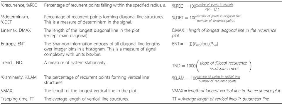
Table 1Summary of quantities used in recurrence quantification analysis. Modified after Webber and Zbilut (2005):https:// www.nsf.gov/pubs/2005/nsf05057/nmbs/nmbs.pdf
%recurrence, %REC Percentage of recurrent points falling within the specified radius,ε. %REC¼100number of points in triangle εðε−1Þ=2
%determinism, %DET
Percentage of recurrent points forming diagonal line structures.
This is a measure of determinism in the signal. %DET¼100
number of points in diagonal lines number of recurrent points
Linemax, DMAX The length of the longest diagonal line in the plot (except main diagonal).
DMAX =length of longest diagonal line in the recurrence plot
Entropy, ENT The Shannon information entropy of all diagonal line lengths over integer bins in a histogram. This is a measure of signal complexity with units bits/bin.
ENT =− ∑(Pbin)log2(Pbin)
Trend. TND A measure of system stationarity.
TND¼1000 slope of%local recurrence vs:displacement
%laminarity, %LAM The percentage of recurrent points forming vertical line
structures. %LAM¼100
number of points in vertical lines number of recurrent points
VMAX The length of the longest vertical line in the plot. VMAX =length of longest vertical line in the recurrence plot
signal. For the Hénon attractor, DMAX = 12 points (Webber and Zbilut 2005).
In addition to the diagonal lines in Fig. 3 which are related to recurrence and determinism, vertical (and horizontal) lines appear on many recurrence plots. These mark transitions in the behaviour of the system. Such transitions may be periodic → periodic
(with a change in frequency), periodic → chaotic or chaotic → chaotic. A vertical line represents an interval where the state does not change or changes relatively slowly but the state of the system changes across the line. A summary of the significance of various patterns on recurrence plots is given in Table 2.
Fig. 2Recurrence quantification analysis (RQA). This diagram shows the steps typically taken in a recurrence nonlinear analysis of a time series together with many of the outputs from the RQA. Modified from Aks (2011)
Recurrence plots and their quantification in this paper have been prepared using the software VRA: http:// visual-recurrence-analysis.software.informer.com/4.9/ and RQA software: http://cwebber.sites.luc.edu/. Other soft-ware is available at http://tocsy.pik-potsdam.de/, http:// tocsy.pik-potsdam.de/CRPtoolbox/, http://tocsy.pik-pots-dam.de/pyunicorn.php and https://www.pks.mpg.de/ ~tisean/.
Prediction and noise reduction
Most signals, especially those from natural systems, contain some form of noise which consists of the addition of a sto-chastic (originates from uncorrelated processes) signal. It is generally considered as an adulteration to the signal and needs to be removed or reduced as far as possible. This no-tion arises from a linear view of the world where the solu-tions to linear differential equasolu-tions are smoothly varying functions and any irregularity must be the result of exter-nally imposed random input. However, irregular behaviour including non-periodicity and intermittency can arise from nonlinear systems with no externally imposed noise. The problem that arises in nonlinear systems is to understand if some of the noise results from deterministic processes of interest and hence should be retained.
Noise is generally classified as white noise with no long-range correlations and coloured noise with some internal structure and long-range correlations (Moss and McClintock 1989). In addition, two different sources of noise can be identified (Grassberger et al. 1993; Kantz 1994; Judd and Stemler 2009). If the behaviour of the system can be expressed at discrete intervals (as in a GNSS lithospheric deformation system) then the se-quence of states,zt, at times,t, can be written
ztþ1¼ f ztð Þ þνt
where the functionfdefines the dynamics of the system
(generally written as set of coupled partial differential equations) and expresses the way in which the system
evolves due to deterministic processes andνtare a series
of independent random variables arising from some process operating in the system. This is referred to as
dynamical noise.
Dynamical noise might be generated in a system where different processes dominate at different time and/or length scales so that some frequencies and/or parts of the system evolve in different ways and rates to others. This results in probability distributions for some time/ length scales diffusing (broadening) and drifting (shifting the mean) with different diffusivities as described by Fokker-Planck equations (Moss and McClintock 1989). Such processes add a stochastic but dynamic noise to the system behaviour but such noise is a fundamental part of the processes operating in the system and should be preserved in any noise reduction algorithm. This kind of noise is generally, but not always, coloured noise (Moss and McClintock1989).
If we make observations,st, at discrete intervals (as in
GNSS time series) then
stþ1¼g sð Þ þt εt
wheregexpresses the state of the system at timetandεt
are independent random variables arising from processes
external to the system and compriseobservational noise.
Such noise may be white or coloured. Any noise reduc-tion process should attempt to reduce the contribureduc-tion from observational noise whilst preserving as much as possible of the dynamical noise. Later in the paper, we give examples of noise reduction for GNSS data and show that some methods preserve the RQA measures of the signal whereas others degrade some deterministic as-pects of the signal.
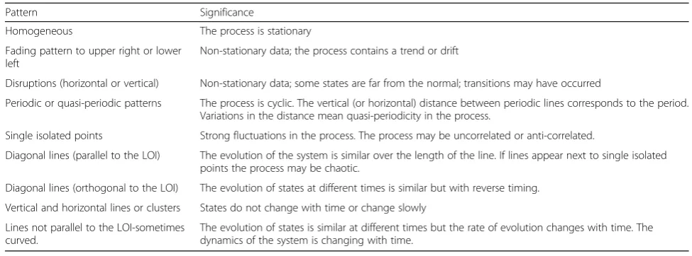
Table 2Significance of patterns in recurrence plots (after Marwan et al.2007a)
Pattern Significance
Homogeneous The process is stationary
Fading pattern to upper right or lower left
Non-stationary data; the process contains a trend or drift
Disruptions (horizontal or vertical) Non-stationary data; some states are far from the normal; transitions may have occurred
Periodic or quasi-periodic patterns The process is cyclic. The vertical (or horizontal) distance between periodic lines corresponds to the period. Variations in the distance mean quasi-periodicity in the process.
Single isolated points Strong fluctuations in the process. The process may be uncorrelated or anti-correlated.
Diagonal lines (parallel to the LOI) The evolution of the system is similar over the length of the line. If lines appear next to single isolated points the process may be chaotic.
Diagonal lines (orthogonal to the LOI) The evolution of states at different times is similar but with reverse timing.
Vertical and horizontal lines or clusters States do not change with time or change slowly
Lines not parallel to the LOI-sometimes curved.
To a large extent, the process of nonlinear noise reduc-tion is the inverse of the nonlinear predicreduc-tion (or forecast-ing) problem. For nonlinear noise reduction, one can determine the dynamics of the system given the whole sig-nal up to its current state and then search for parts of the signal in the past that are not part of the dynamics. These parts are removed as noise. This means we take the whole signal and work backwards. For prediction, we take one part of the signal, determine the dynamics and then see if we can find a part of the dynamics that fits the way in which the signal is evolving into the future and use that to make a forward prediction or forecast. Nonlinear predic-tion is particularly useful if one needs to“fill in”short gaps in data sets in a manner that honours the deterministic dynamics of the system.
An approach to prediction in chaotic systems is spelt out here based on Casdagli and Eubank (1992), Weigend and Gershenfeld (1994), Fan and Gijbels (1996) and Abarbanel (1996). To predict a pointxn+ 1, we determine the last known state of the system as represented by the vector X¼½xn;xn−τ;xn−2τ; :……;xn−ðD−1Þτ, where D is the embedding dimension andτis the delay. We then search the series to find k similar states that have occurred in the past, where “similarity” is determined by evaluating the distance between the vector X and its neighbour vectorX’in theD-dimensional state space. The concept is that if the observable signal was generated by some deterministic map, M:ð:…ððxn;xn−τÞ;xn−2τÞ;…;xn−ðD−1Þτ Þ ¼xnþ1; that map can be reconstructed from the data by looking at the signal behaviour in the neighbourhood of X. We find the approximation of M by fitting a low-order polynomial (Fan and Gijbels 1996) which maps k nearest neighbours (similar states) of X onto their next immediate values. Now, we can use this map to predictxn+ 1. In other words, we make an assumption that M is fairly smooth aroundX, and so if a state X0¼½
x0n;x0n−τ;x0n−2τ;…;x0n−ðD−1Þτ in the neighbourhood of X resulted in the observation, x’n+ 1, in the past, then the point xn+ 1 which we want to predict must be some-where nearx’n+ 1. In any chaotic system, we expect the error in prediction to increase exponentially (as mea-sured by the Lyapunov exponent) as we move away from known data.
The above approach is based on intensive work on prediction in chaotic systems largely carried out in the 1990s and relies on finding local states in the past that resemble current states of the system. A relatively recent approach to nonlinear filtering is the shadowing filter
(Stemler and Judd 2009). A shadowing filter (Davies 1993; Bröcker et al.2002; Judd2003; Judd2008a,2008b) searches in state space for atrajectory (defined by a se-quence ofztfor the system), rather than local states, that
remains close to (that is, the trajectory shadows) a
sequence of observations,st, on the system. The algorithm
is discussed by Judd and Stemler (2009). We do not use a shadowing filter in this paper, but its use in future work promises to give better results than reported here.
Synchronisation
Of particular interest in systems where many coupled episodic sub-systems are operating, such as in GNSS and seismic systems, is to see if the sub-systems influ-ence each other so that some form of spatial or temporal synchronisation occurs. Such synchronisation can be of five forms (Romano Blasco2004; Marwan et al.2007a):
Phase synchronisation: the two signals are phase
locked but amplitudes are not identical.
Frequency synchronisation: the two signals are
frequency locked.
Lag synchronisation: there is a time or space lag
between similar or identical states.
Generalised synchronisation: the synchronisation
comprises nonlinear locking between similar or identical states.
Chaotic transition synchronisation: similar behaviour
in the signal is locked into chaotic transitions in the respective recurrence plots that occur at similar times in two or more time series.
In many systems, synchronisation switches from one of these five types to another as the system evolves and the coupling between parts of the system changes strength (Romano Blasco 2004). We will see that cross recurrence plots and particularly joint recurrence plots
are powerful ways of investigating such synchronisation (Marwan et al.2007a). Just as a recurrence plot identifies recurrences at different parts of the same signal, cross recurrence plots identify recurrences at identical times on two different signals. In other words, a cross recur-rence plot identifies those times when a state in one sys-tem recurs in the other. Joint recurrence plots identify recurrences in the recurrence histograms of two signals; they are somewhat similar to identifying simultaneously occurring maxima in power spectra from two different signals in linear systems. Clearly, the plots only reflect something of the dynamics if both signals originate from similar processes and belong to state spaces with similar or identical attractors.
By analogue with (4) a cross recurrence matrix for two time seriesxiandyjis defined as
CRij¼Θ ε−xi−yj
for i¼1;Nand j¼1;M
JRij¼Θ εx−xi−xj
Θ εy− y i−yj
for i;j¼1;N
where εx and εy are tolerances for the individual time
series. For joint recurrence, JRij= 1 if ‖xi−xj‖<εxand
‖yi−yj‖<εy otherwise JRij= 0. Joint recurrence
mea-sures the probability that both the xi and yj systems
revisit simultaneously the neighbourhood of a point in their respective phase spaces previously revisited The equivalent of an RQA analysis can be conducted for each of these matrices, CRQA and JRQA respectively but in some instances the measures may have limited use
(Romano Blasco2004). For instance in a cross recurrence
plot for two signals with different frequencies (see Fig.4b
below), there may be no diagonal lines so that measures such as %DET and DMAX have little meaning. Romano
Blasco (2004) shows that the entropy in particular is a
use-ful measure for studying synchronisation in joint recur-rence plots. In general, cross recurrecur-rence is not a useful way of analysing synchronicity between two systems
(Romano Blasco2004) but we use aspects of cross
recur-rence plots below as a useful way of portraying synchron-isation between signals from two GNSS stations.
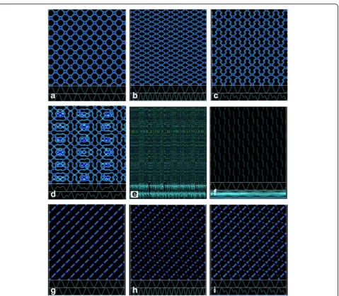
In Fig.4, we show several different cross and joint re-currence plots so that the reader might obtain some insight into how to read such plots. In Fig. 4a recur-rences between the signals y= sin(x) and y= cos(x) are plotted. The recurrences plot on straight diagonal lines and the vertical distance between these lines is the (iden-tical) period of both signals. The straight diagonal lines are referred to (Marwan et al. 2007a) aslines of identity
(LOI). In a more general recurrence plot for a dynamical system, the LOIs represent segments of the trajectories of both systems that run parallel for some time. The fre-quency and lengths of these lines are measures of the similarity and nonlinear interactions between the two systems.
Figure 4b is a cross recurrence plot between the two signals y= sin(x) and y= sin(2x). The LOIs are now in-clined at β= tan−1(1/2) = 26.6° to the horizontal axis. The slope,β, is given by Marwan et al. (2007a)
β¼ tan−1 ∂
∂t T1
T2
ð5Þ
whereT1andT2are the time scale characteristic of the
two systems.
In Fig. 4c, recurrences between y= sin(x) and y= sin(x) + sin(5x2) are plotted. The straight LOIs of Fig.4a, b are now curved and are referred to as lines of syn-chronisation(LOSs). Thus, the details of the cross recur-rence plot can give information on whether the signals that are compared are linear or nonlinear and also give an indication of both the absolute and the relative time scales associated with the two systems. Figure 4d is a
cross recurrence plot between the two quasi-periodic signals: y¼ sinðxÞ þ sinðp2ffiffiffixÞ and y= sin(x) + sin(πx). Figure4eis a cross recurrence plot between two logistic signals given by xn+ 1=αxn(1 +xn) with α= 3.7 and 3.8
and Fig.4fis a joint recurrence plot between the signals:
y= sin(x) andy= sin(20x).
Plotting the changes in slopes of LOSs is a powerful way of tracking the evolution of two synchronised sys-tems and of observing the ways in which time scales that characterise each system change with time.
Examples of joint recurrence plots are given in Fig.4g, h, ifor the same signals in the cross recurrence plots of Fig.4a, b, c. In contrast to the cross recurrence plots (a to c) which express the ways in which two signals oc-cupy similar states synchronously, a joint recurrence plot expresses (in the form of blue lines or dots in g to i) the ways in which recurrences on two different signals occur synchronously.
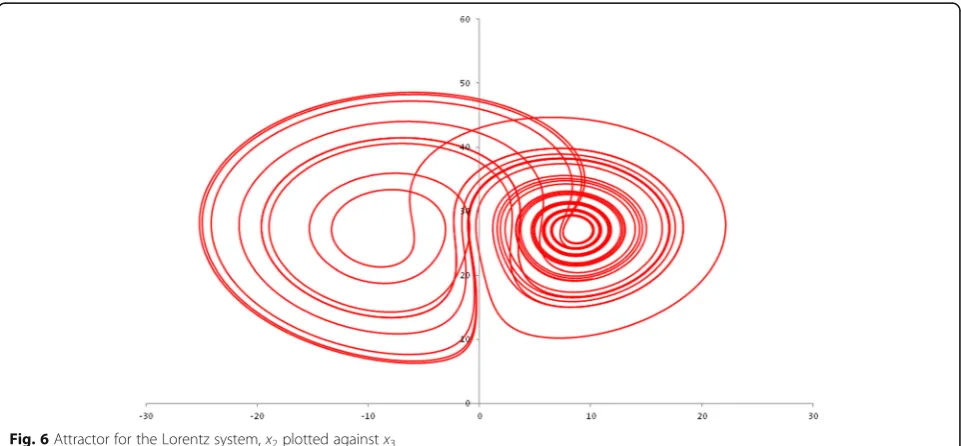
An example: the Lorentz attractor—quantification and prediction
As an example of the principles involved in nonlinear analysis and prediction, we present a discussion centred on the relatively simple, low-dimensional Lorentz at-tractor (Sprott 2003, pp. 90–92) which forms the basis for modern weather forecasts (Yoden2007). This system is described by the set of differential equations:
dx1
dt ¼−
3
2Px1þ
2
3aPx2
dx2
dt ¼ax1x3−
3
2x2þaRx1 ð6Þ
dx3
dt ¼−
1
2ax1x2−4x3
where x1, x2 and x3 are variables of interest, t is time
and a,Pand Rare parameters of the system. The signal
that results for x1from these equations with a= 2.25, P
= 20/3 and R=−4/9 is given in Fig. 5a with the
multi-fractal spectrum in Fig.5b. The well-defined multifractal
spectrum arises because the Lorentz system is chaotic and, in principle, its attractor consists of an indefinite number of singularities with variable densities of
occur-rence,α, on the attractor (Beck and Schlögl (1995). The
multifractal spectrum expresses the density distribution,
f(α), of these singularities as a function of their strength,
α(Arneodo et al.1995).
embedding dimension (Fig. 7b) and the percentage of false neighbours against embedding dimension (Fig. 7c). The estimated dynamical dimension for the Lorentz at-tractor is 2.1736 whereas Fig. 7b, c would suggest an embedding dimension of ≈2. Thus, it is not necessary for the attractor to be known for a system, its embed-ding dimension and its topology can be estimated from
the recurrence plot. This dimension is important for constraining any data model that is constructed.
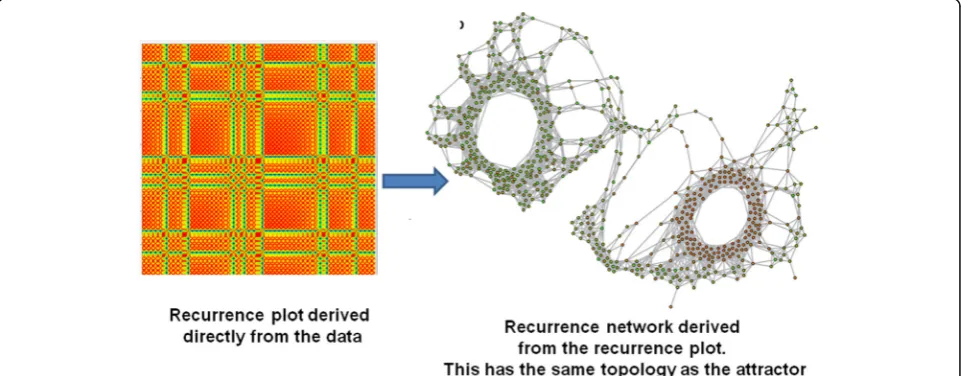
Although we will not explore recurrence networks in this paper we mention, for completeness, that a network with the topology of the attractor can be calculated from the recurrence plot (Donner et al. 2010; McCullough et al.2017) as shown in Fig.8. The adjunct matrix, Aij, for
Fig. 4Cross and joint recurrence plots.aCross recurrence plot between sin(x) (upper trace) and cos(x) (lower trace). High recurrence is represented by the dark blue (straight) lines of synchronisation at 45oto the horizontal axis.bCross recurrence plot between sin(x) (upper trace) and sin(2x) (lower trace). High recurrence is represented by the dark blue (straight) lines of synchronisation at tan−1(1/2) = 26.6° to the horizontal axis. The ratio ½ is the ratio of the frequencies of the two signals.cCross recurrence plot between sin(x) (upper trace) and sin(x) + sin(5x2) (lower trace). High recurrence is represented by the (curved) dark blue lines of synchronisation. The local slope of the line of synchronisation is the arctangent of the ratios of the local frequencies of the signals.dCross recurrence between two quasi-periodic signals:y¼ sinðxÞ þ sinðp2ffiffiffixÞ(upper frame),y= sin(x) + sin(πx)(lower frame).eCross recurrence plot between signals from two logistic equations,xn+ 1=αxn(1−xn), withα= 3.7 (upper frame) andα= 3.8 (lower frame).
the network is related to the recurrence matrix in (4) by Aij= Rij−δijwhereδijis the Kronecker delta. Recurrence
network software is available at
http://tocsy.pik-pots-dam.de/pyunicorn.php and needs to be used in
conjunction with a graphical network code such as Gephi https://gephi.org/. Recurrence networks have been applied to seismic time series by Lin et al. (2016). We revisit the concept of nonlinear networks in the “Discussion”section as a basis for monitoring the behav-iour of GNSS data networks.
The application of nonlinear noise reduction to the Lorentz system is shown in Fig.9where one can see that the prediction is still very good 450 steps away from a 3000-step training set but is rising exponentially by the end of the prediction. In plots such as these, the
normalised error is that relative to that which would be expected from a linear prediction of the mean expressed as the normalised mean squared error, NMSE, discussed in Weigend and Gershenfeld (1994) and defined as
NMSE¼ 1
σ2N
XN
i¼1
xi−^xi
ð Þ2 ð
7Þ
where xi is the observed value of the ith point in a
series of length N, ^xi is the predicted value and σ is
the standard deviation of the observed time series
over the length, N. NMSE is the ratio of the mean
squared errors of the prediction method used to a
method that predicts the mean at every step. In Fig. 9,
this ratio is a maximum of ≈0.0065.
Fig. 5Features of the Lorentz system.ax1signal from Lorentz signal with parameters given in the text.bMultifractal spectrum from
Lorentz system
Significance of a linear trend in the data
An issue that arises in the nonlinear analysis of GNSS data is the significance of any linear trend that com-monly exists in the data and of the effect of removing this trend. Consider a pair of time series, xiand yj,with
i= 1, N andj= 1, M and a pair of derived time series,^xi;^yj, where ^xi¼xiþat and y^i¼yiþbt where a and b are constants andtis time. Then,xi,yjare time series derived
from ^xi;^yj by removal of a linear trend. For the cross re-currence plots of these pairs of time series to be identical,
Θ ε−xi−yj
¼Θ ε−^xi−^yj
for i¼1;Nand j¼1;M
This condition can be satisfied ifðkxi−yjkÞ ¼ ðk^xi−^yjkÞ
foralli¼1;Nand j¼1;M but in general this will be a difficult condition to satisfy. Similarly joint recurrence
Fig. 7Recurrence plot and embedding dimension for the Lorentz system.aRecurrence plot. The colour code to the side ofaindicates thatε/c varies from 0 to 76.bCorrelation dimension plotted against embedding dimension. The plot departs from a slope of 45o(equivalent to white noise) at an embedding dimension of 2 giving an estimate for the true embedding dimension of the attractor.cPercentage of false nearest neighbours plotted against embedding dimension. The minimum is at 2 indicating again that this is close to true embedding dimension for the system. The theoretical value of the dynamical dimension is 2.17
plots for the time series ^xi;^yj will be identical for that of the pair^xi;^yjif
Θ εx− xi−x j
Θ εy− y i−yj
¼ Θεx−xi^−^xjΘ εy− ^y i−^yj
for i;j¼1;N
Again, in general this condition will be difficult to satisfy. As an indication of the differences that may arise, Fig. 10 presents cross recurrence plots for two quasi-periodic signals. Figure 10a is for these two signals with no linear trend whilst Fig. 10b is for the same two signals with a linear trend added to the first. One can see that the two plots are quite different. In some instances, however, the re-moval of a linear trend makes quite small differ-ences as we will see for the KAIK_e signal later in the paper.
Analysis of GNSS data
Nature of the data
Time series for crustal displacements using satellite ac-quired data are collected by the GeoNet organisation in
New Zealand, a collaboration between the NZ Earth-quake Commission and GNS Science, using GNSS (popularly known as GPS) receivers and antennae. In order to explore the application of nonlinear time ana-lysis to GNSS data, we have selected five of the operat-ing GNSS stations shown as yellow triangles in Fig.11a. At each station, three output files are available contain-ing displacement records relative to a reference datum (Hofmann-Wellenhof et al. 2008) defined by the Inter-national Terrestrial Reference Frame (ITRF2008) for East, North and vertical displacements evaluated on a daily basis from data collected every second. The 1 s data contain noise from known and unknown sources and may be influenced by both deterministic and observational noise produced by the processes of data collection (Hofmann-Wellenhof et al. 2008). In these procedures, linear combinations of various signal fre-quencies are combined as a method of smoothing the 1 s data (Hofmann-Wellenhof et al. 2008). In addition, the 1 s data are aggregated from 1 s to 1 day time series. We have retained the raw supplied data, expressed as daily displacements with no further processing, since in any nonlinear analysis, it is never clear initially what is noise from measurement or other external sources (ob-servational noise) and how much of the signal is
intrinsic to the nonlinearity of the dynamics (dynamical noise). It would be interesting to begin with the 1 s data in future work. An initial exploration, as this study is, should retain as much of the data as possible with a view to identifying externally induced (non-deterministic) noise at a later stage. A brief look at noise in these sig-nals is given later in the paper. Some of the possible lin-ear methods of noise reduction are considered in Goudarzi et al. (2012). At each station, data are collected for the easterly (suffix: _e), northerly (suffix: _n) and vertical (suffix: _u) displacements. In Fig. 11, we show only the easterly component data except for the sta-tions CNST and PAWA where we explore the vertical component data. We also explore possible synchron-isation between nearby stations using cross- and joint-recurrence plots. Since there is some interest in understanding synchronisation between two stations on the North Island of New Zealand with an event (marked as a red triangle in Fig. 11a) on the South Island (Wallace et al. 2017), we also explore syn-chronisation between two distant stations.
The raw data used here and reported at 1 day inter-vals contains relatively small gaps (about 6 days at most in the signals we investigated) that presumably arise from station down-time. We have retained these gaps for most analyses but have explored the effect of removing them. Such a process seems to make little difference to the details of both recurrence and cross recurrence plots but clearly is important if one wants to match events in cross and joint recurrence plots. Future work should explore nonlinear prediction methods in filling these gaps.
The emphasis in the use of GNSS time series for geo-tectonic purposes in most published literature is to es-tablish the velocity imposed on the crust by plate tectonic processes. As such the data are processed
(Beavan and Haines 2001; Wallace et al. 2004) in order to arrive at a velocity field that is smooth and continu-ous over substantial parts of the surface of the Earth. From such studies, important constraints can be placed on that part of the deformation of the crust that is com-monly referred to as the rigid body motions (Wallace et al. 2004, 2010). Many studies propose that the crust is made of microplates that may have slightly different rigid body motions (Thatcher 1995, 2007; Chen et al. 2004; Wallace et al.2004,2010) and although some may offer more continuous models (Zhang et al. 2004) the case for such micro-plates existing in New Zealand seems to be well established (Wallace et al. 2004,2010). The deformation within such microplates is commonly thought of as elastic (McCaffrey 2002; Wallace et al. 2010) and such an assumption is reasonable if one is seeking a smooth, continuous distribution of velocities on the scale of the microplate. However, in this paper, we seek to understand something of the system dynam-ics of crustal deformation processes by examining the history of deformation, continuous and discontinuous,
within these microplates together with the coupling be-tween these microplates over time. As such, the rigid plate tectonic motions are, in a sense, noise as far as the signal is concerned whereas for geotectonic purposes the details of the signal, which are our interest, are noise that is commonly removed by intensive processing (Wallace et al.2010).
The rigid body motions of the crust arising from plate tectonic motions constitute a vector field on the surface of the Earth whereas the history of displacements within a microplate can be represented as an attractor that de-scribes the dynamics in phase space. In principle, the characteristics of the attractor should not be altered by the subtraction of rigid body velocities but there is an issue in defining how much of an observed trend in a
GNSS signal arises from a rigid body motion is a contri-bution from regional plate tectonic motions and how much arises from elastic deformation or even from other internal permanent plastic/viscous deformation of the microplate. This is particularly the case if the overall trend is not linear.
For the recurrence plots presented here, we have elected not to remove the overall trend since the RQA measures for such plots are influenced by the trend although the trend, if pronounced, is clear in the plot. This is particu-larly true for KAHU_e and PAWA_e (Fig. 11e, f, but for other plots, the influence of the trend is minimal. We have removed the trend from the KAIK_e plot when we exam-ine synchronisation between stations but recognise that such removal may have an influence on the apparent dy-namics of the system; we examine the influence of such trend removal later in the paper.
It would seem from a cursory examination of many of the GNSS records from the North and South Islands of New Zealand that New Zealand is composed of an inter-locking mosaic of blocks and within each block the history of GNSS displacements have a similar history. It appears that each block moves whilst maintaining de-formation compatibility at the boundaries of these blocks by combinations of boundary slip, block rotation and internal elastic, brittle and plastic deformation. There is evidence (Wallace et al. 2017 and this paper) that the motions of individual blocks are synchronised with others over quite large distances. The question arises therefore: How much of the average trend is to be attributed to the overall plate tectonic motions and how much is to be attributed to the nonlinear dynamics of the microplate? Although such a question is fundamen-tal and is in need of detailed examination we elect to side-step the issue and unless indicated otherwise treat the raw data as an input to analyses.
Recurrence analysis of GNSS data
We begin by analysing the data from one station (CNST) in some detail to illustrate the procedures spelt out in Fig.2and then proceed to examine the other four other stations shown as yellow triangles in Fig. 11a in less detail. We then proceed to examine nonlinear syn-chronisation of displacement histories between stations CNST and PAWA, a distance of≈220 km, and between stations CNST, PAWA and KAIK, a distance of≈440 to 650 km.
In all the recurrence/cross-recurrence/joint-recurrence plots for GNSS data, the embedding dimension is 10 and the time delay is 5. The scaling is maximum dis-tance, and the radius is 20% (Webber and Zbilut2005). The parameterc is 5 so that four levels of contours ap-pear in each plot. The signal for the raw data together with the time scale is shown at the base of each
recurrence plot at the same linear scale as the plot. Cross reference to Fig.11gives finer detail of the abso-lute time scale for each plot.
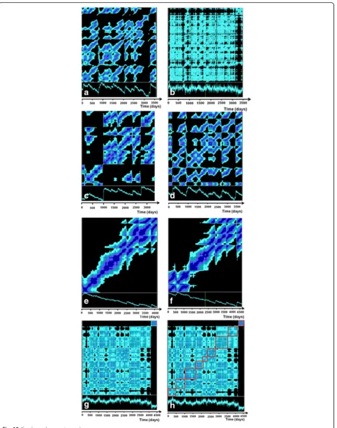
Figure12a, bshows the recurrence plots and associated signals for the raw daily data for CNST_e and CNST_u. We have not analysed CNST_n data. The contrast in ap-pearance between Fig.12a, breflects the nature of the two signals. The CNST_e data comprise a number of discon-tinuities with downward non-stationary trends between discontinuities. This is represented on the recurrence plot by abrupt gaps in recurrence (black areas) with fading to the upper right patterns between gaps. The large black areas (up to≈300 days wide) where no recurrences occur are particularly evident immediately prior to large discon-tinuities in the displacement record.
The recurrence plot for CNST_u (Fig. 12b) is much more highly populated with recurrences. Regions of no recurrence (black) tend to occur immediately prior to changes in the patterns in the raw data but these gaps are ≈50 days wide as opposed to up to a year in the CNST_e recurrence plot.
The essential attributes of the CNST_e recurrence plot are expressed in the RQA analysis of Table 3. The rela-tively low level of %REC is expressed by the high propor-tion of black areas in Fig. 12a. The signal is highly deterministic as indicated by the high values of %DET. DMAX is large which indicates a small value for the first Lyapunov exponent; this in turn indicates the potential for good predictability. The entropy (ENT = 4.4 bits/bin) is larger than that of the Hénon system (ENT = 2.56 bits/bin) and so suggests predictability may be more dif-ficult for CNST signals than for the Hénon system.
These values of RQA measures for CNST_e are to be contrasted with those for CNST_u which reflects the more diffuse nature of the latter signal. In particular, the first Lyapunov exponent indicates that predictability may be difficult.
Similar observations to the above hold for the other sig-nals examined: large gaps (black areas) in recurrence tend to occur prior to large discontinuities in displacement, de-terminism is high and the first Lyapunov exponent is small. Obvious differences in *_e recurrence plots exist for data sets that show significant non-stationarity: recurrence tends to be restricted to a relatively narrow zone either side of the main diagonal LOI but again discontinuities in the signal are preceded on the recurrence plots by gaps in recurrence.
is known as a sliding window analysis (Webber and Zbilut 2005).
Embedding dimension and the nature of the attractor
In Fig. 13, we show plots of the correlation dimension, given by (3), and the percentage of false nearest
neigh-bours against embedding dimension for CNST_e
(Fig. 13a, b) and CNST_u (Fig. 13c, d). The correlation dimension plot tends to deviate from a straight line somewhere in the range 8 to 10 indicating a relatively high value for the embedding dimension. This indicates that the underlying dynamics of the system involve 8 to 10 state variables; certainly more state variables are in-volved than in the Lorentz system (5). The percentage of false nearest neighbours gives little useful information as far as the embedding dimension is concerned and continues to decrease as the embedding dimension increases. This again indicates that the attractor is complicated and that it is difficult to view the attractor in its true embedding dimension with the data available. More data are needed to cover the attractor and sample all possible states.
In Fig. 14, we show a projection of the attractor for the CNST_e data set shown in Fig. 11b. As indicated earlier, the embedding dimension for this attractor is probably about 10 so Fig. 14 is a projection from this
10-dimensional state space into three dimensions. The fact that many trajectories cross each other in this pro-jection is an indication of the large number of false neighbours in three dimensions. Also note the presence of knot-like “outliers” in the system that are visited rarely but have a complicated shape with false neigh-bours in three dimensions. This indicates that the local estimates of the embedding dimension can be quite vari-able (Small 2005) and we tentatively assume that these complications in the attractor are responsible for any difficulties involved in using false nearest neighbours as a means of estimating the embedding dimension.
Noise reduction
As an example of the differences between nonlinear and linear noise reduction procedures, we first present in Fig. 15 two examples of the nonlinear noise reduction procedure discussed earlier in the paper. Here, the embedding dimension is taken as 10 and the delay, 5. Figure 15a shows approximately 76% noise reduction and the corresponding plot of correlation dimension against embedding dimension is shown in Fig.15b. This shows a reduction in the possible embedding dimension to about 5. In Fig.15c, 80% noise reduction is shown for CNST_u and the corresponding plot of correlation di-mension against embedding didi-mension is shown in Fig. 15d with a slight reduction in the indicated
(See figure on previous page.)
Fig. 12Recurrence plots for stations marked as yellow stars in Fig.11a. In all figures the embedding dimension is 10 and the time delay is 5. The scaling is maximum distance and the radius is 20% (Webber and Zbilut2005). The parametercis 5 so that 4 levels of contors appear in each plot. The signal for the raw data is shown at the base of each recurrence plot at the same linear scale as the plot. Details of these signals together with the time scale are shown in Fig.11.aCNST_e.bCNST_u.cPARI_e.dMAHI_e.eKAHU_e.fPAWA_e.gPAWA_u.hPAWA_u with sliding windows marked in red. Within each window a different pattern of recurrence occurs. The zero for the time scale in each of these plots and in subsequent plots in this paper is the zero for the relevant time scale in Fig.11
Table 3RQA measures for selected GNSS data sets on the North Island of New Zealand
Station Data set %REC %DET DMAX ENT TREND %LAM VMAX TTIME
CNST e 39.49 97.88 3588 4.4 −6 98.5 837 51.56
CNST* e_trunc 38.44 97.48 2687 4.28 −7.05 98.21 411 40.1
CNST** e_trunc_n 36.44 97.48 2688 4.28 −7.02 98.21 411 40.11
CNST*** e_reg_n 36.48 97.31 2676 3.8 −10.02 97.99 446 31.85
CNST u 6.9 29.13 45 0.89 −1.92 45.88 42 2.59
CNST**** u_n 27.77 65.81 114 1.6 −6.95 76.54 154 3.58
PARI e 39.26 98.73 3380 4.5 −13.77 99.07 898 70.36
MAHI e 42.38 98.26 3685 4.38 −9.77 98.79 841 60.7
KAHU e 37.47 99.47 4183 4.51 −27.64 99.62 1315 181.64
PAWA e 38.16 99.50 4526 5.14 −25.24 99.65 1326 200.18
PAWA u 56.32 95.54 1796 2.92 −15.05 96.76 1027 18.05
*CNST_e data truncated from 3650 days to 3300 days **Truncated CNST_e data with nonlinear noise removal
embedding dimension compared to Fig.13c. An attempt was made to optimise the noise reduction in these two cases by exploring different embedding dimensions and delays.
In Table4, the RQA data are shown for CNST_e (raw data, column 1), CNST_e with nonlinear noise reduction (column 2) and CNST_e with noise removed by the lin-ear regional filter described by Beavan et al. (2004); this latter method of noise removal has now been discontin-ued by GeoNet. The nonlinear noise removal process leads to no or insignificant changes in the RQA mea-sures whereas the regional filter method produces 5% in-crease in %recurrence, an 11% inin-crease in entropy, a 42% decrease in trend and a 21% increase in trapping time. Thus, although the data may appear “smoother”, the basic measures of the dynamics of the system have been significantly altered by the linear filtering method. A basic premise is that any data reduction method should preserve dynamic noise and it seems that the linear method has removed some such noise in this example.
Sliding window analysis of CNST_e data
A useful way of analysing recurrence plots is called the
sliding window method (Marwan et al. 2007a) whereby the recurrence plot is divided into small windows along the main diagonal LOI which may or may not overlap as desired (Fig. 12h). RQA measures are produced in each window enabling plots of these measures to be made through the history of the time series. In Fig. 16,
Fig. 13Correlation dimensions (left hand frames) and false nearest neighbour (right hand frames) plotted against embedding dimension.a,b Data set: CNST_e.c,dData set: CNST_u
Fig. 14Projection of the attractor for CNST_e data from a higher
such an analysis is shown for CNST_e data. This enables the RQA data to be compared directly with local patterns in the raw data. In particular, we are interested in RQA measures that may serve as precursors to the main dis-continuities in the displacement record.
In this analysis, the window size is 100 days and there is a 50 day overlap between windows so that each win-dow can“see”100 days ahead; this represents two black dots on the RQA signals shown in Fig. 16. Each dot is plotted at thebeginning of the 100 day window so each dot represents the RQA measure of the signal 100 days ahead. Here, we concentrate on the main displacement discontinuity that begins about day 3307 and continues until about day 3320. One can see that the mean and
standard deviation track the signal precisely and so are of little use as precursors. However, the %LAM and DMAX measures both behave anomalously 100 days be-fore the displacement discontinuity at ~ 3307 days and so are candidates as precursors for this event although it is appreciated that this event is not sharp and extends in a compound manner starting at ≈3200 days; others are possible but higher resolution (say 0.1 day binning) is necessary before one can be definitive.
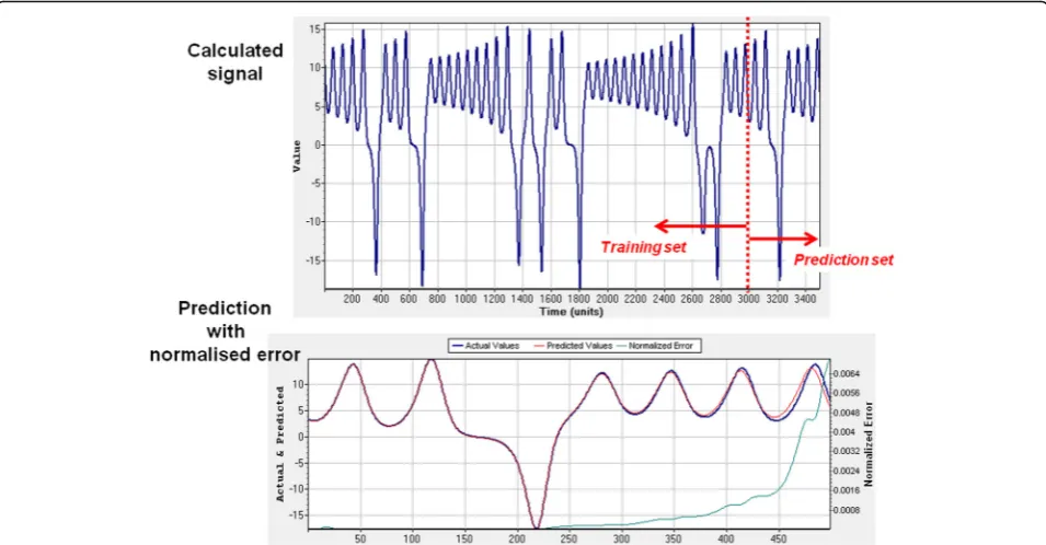
Nonlinear prediction of CNST_e data
A test of whether one has a reasonable data model is to attempt some form of nonlinear prediction. We have attempted this for the CNST_e data set using the first
Fig. 15Nonlinear noise reduction for CNST data sets. In left hand panels blue is original signal and red is the signal after noise reduction.aNoise reduction for CNST_e; 76% noise reduction.bPlot of correlation dimension against embeddding dimension for CNST_e after noise reduction. This should be compared to Fig.13a.cNoise reduction for CNSTE_u; 80% noise reduction.dPlot of correlation dimension against embeddding dimension for CNST_u after noise reduction. This should be compared to Fig.13c
Table 4Comparison of RQA measures for data set CNST_e, as raw data (column 1), with nonlinear noise reduction (column 2) and with noise reduction using the regional filter method (column 3; Beavan et al.2004)
Data set 1. CNST_e Raw one-day data
2. CNST_e
Nonlinear noise removal
3. CNST_e Regional filter
% change of # 2 with respect to 1 % change of # 3 with respect to 1
%REC 38.44 38.44 36.48 0 5.10
%DET 97.48 97.48 97.31 0 0.17
LMAX 2687 2688 2676 −0.04 0.41
ENT 4.28 4.28 3.8 0 11.21
TREND −7.05 −7.02 −10.02 −0.43 −42.13
%LAM 98.21 98.21 97.99 0 0.22
VMAX 411 411 446 0 −8.52
3200 days of the signal as a training set and an attempted prediction for the period 3201 to 3501 days. The results are shown in Fig. 17 which represents the 300 days starting at day 3201 and ending at day 3500 for an embedding dimension of 10, a delay of 10, a local lin-ear weight predictor and a Gaussian kernel. The actual values are plotted in blue and the prediction in red. The normalised error (in green) starts high at ≈1.4 remains high and drops to below 1 at the main jump in displace-ment. The final normalised error is ~ 0.98 but is still marginally better than linear predictors based on (7). The predicted signal hugs the details of the observed data quite nicely including the large displacement at about 105 days. This analysis again confirms that the embedding dimension of the attractor is relatively large. Reducing the embedding dimension below 10 or increas-ing the embeddincreas-ing dimension to 12 give normalised er-rors far greater than 1.
Synchronisation of data sets
It is clear that some of the large displacement events in New Zealand occur at near to the same time. Thus the same large displacement events can be observed syn-chronously at several stations (Wallace et al.2017, Fig.2). This represents synchronisation of large displacements over distances of at least 220 km. Recently, Wallace et al. (2017) have proposed that the magnitude 7.8 seismic Kaikōura event triggered large displacement events 250 to 600 km away on the North Island for 1 to 2 weeks after the South Island event. Whilst such synchronisa-tion is clear, it is of interest to see if more subtle forms of synchronisation exist and, if so, over what length and time scales does synchronisation occur? Also an under-standing of where such synchronisation sits in the classi-fication of synchronisation types described earlier in the paper and details of the frequencies at which synchron-isation occurs would shed light on the dynamics of crustal deformation. In what follows, we employ cross-recurrence and joint recurrence plots to detect
synchronisation between stations, to clarify details of the synchronisation and to classify the mode of synchronisation.
Synchronisation between stations on the North Island
In Fig. 18, we show synchronisation between signals for CNST_e and PAWA_e. Figure18a is a cross recurrence plot and shows that gaps in synchronisation between the two signals (black areas on the cross recurrence plot marked by white arrows) begin months before major dis-placement events at both CNST and PAWA, and syn-chronisation begins again immediately after an event. The ratio of recurrence time scales for the two stations,
TCNST/TPAWA, is ≈3:5 as shown by the slope of the LOSs and using (5). There are places in Fig.18ajust be-fore large displacement events where the LOS is almost horizontal indicating that TCNST/TPAWA switches from
≈3:5 to a large number (β in (5) approaches 0o as
TCNST/TPAWA →∞). These places (marked with red ar-rows) of lowTCNST/TPAWAcorrespond to discontinuities in the CNST_e displacement plot. Discontinuities in the PAWA_e displacement plot correspond to discontinu-ities in the LOSs with no change inTCNST/TPAWA.
The joint recurrence plot is shown in Fig. 18b and shows a high degree of joint recurrence along a single LOS for the early part of the history and widens out to have a higher proportion of joint recurrences as the major event is approached. After the major event, the joint recurrences are still strongly synchronised but the pattern of joint recurrences has broadened even further.
Figure18c, dshows the probability of a recurrence ver-sus frequency (1/lag in days) for CNST_e and PAWA_e respectively. Both signals have fractal distributions with respect to time lag for low frequencies but are more or less independent of frequency at high frequencies which is where the majority of recurrences occur and where the power in the signal exists. The details of the distributions are quite different for the two stations indicating that no simple phase or frequency locking exists between these
two stations. Figure 18e shows the scaling on a log-log plot of the probability of a joint recurrence against fre-quency (both normalised). The relation indicated by the dotted line is:
normalised recurrence probability is proportional to
(normalised frequency)11.6
indicating that all of the power in the signal is parti-tioned into the highest frequencies. Since almost all (99%) of the joint recurrences occur in the four or five highest frequencies in Fig.18e, the partitioning of power into the highest frequencies is far more pronounced (as indicated by the dotted red line) than indicated by the above scaling relation. These observations indicate that the synchronisation between CNST and PAWA is a form of generalised synchronisation.
Synchronisation between stations on the North Island and KAIK on the South Island
The spectacular observations of Wallace et al. (2017) that the magnitude 7.8 Kaikōura seismic event in the South Island of New Zealand is followed for a few weeks by slow displacement events 250–600 km distant on the North Island indicates clear lag synchronisation over large distances. The questions we want to address are the following: do other forms of synchronisation exist over these large distances and, if so, what form do they take and is there information in the form of pre-cursors in the synchronisation patterns? We first char-acterise the KAIK displacement history using a sliding window with RQA and then investigate cross recur-rence plots between CNST and KAIK and between PAWA and KAIK.
Figure 19 shows the results of a sliding window ana-lysis for the KAIK_e signal over a time period identical for signals from CNST and PAWA. The Kaikōura event occurs at day 3317 and so this event in Fig. 18is in the 50 day window following the red star in each RQA plot. The window is 100 days wide and the overlap between windows is 50 days. This means that each black dot in Fig. 19can “see” two black dots ahead. The RQA mea-sures for the 100 day wide window are plotted at the day corresponding to the beginning of the window. Any precursors for KAIK_e events must therefore be evi-dent two dots or more before the red star. A measure is deemed useful as a precursor to an event if the measure rises to more than twice the mean of the total signal for that measure for the period of 100 days before the event.
We see that the following RQA measures are not suit-able as precursors to the Kaikōura event: mean, standard deviation, TTIME and TREND. The other RQA mea-sures %REC, %DET, DMAX, ENT, %LAM and VMAX
seem to be useful precursors and increase to well over the mean of the measure 100 days before the Kaikōura event. These measures are connected to the determinism and the organisation of recurrence states and indicate that the processes operating in the system are becoming more organised for about 3 months at least before the Kaikōura event. The question then arises: do stations in the North Island“know”about this organisation process?
Figure 20 shows cross and joint recurrence plots for *_e time series between PAWA and KAIK. Figure 20a indicates strong synchronisation between PAWA and KAIK at punctuated intervals for a decade before the Kaikōura event. The ratio of time scales,TPAWA/TKAIK, as indicated by the dark blue LOSs in Fig.20a and from (5) is approximately 1:1 over large portions of the history but locally as in Fig. 20d the ratio increases to large values possibly > 20 at places indicated by the red arrow. Figure 20c shows that the ratio has increased to 3–5 before the main Kaikōura event. These relations presum-ably reflect a form of generalised synchronisation. Figure 20b shows synchronisation of joint recurrences over a narrow range of recurrences for the same period as is shown in Fig.20a.
Figure 21 shows strong synchronisation between CNST and KAIK at punctuated intervals over a period of ~ 3000 days with TCNST/TKAIK large but not easily quantified. If the ratio of the time scales is≥11 then the slope of the LOSs is≥85° so that the LOSs in Fig.21 in-dicate that (TCNST/TKAIK)≥11 and probably closer to 20. Figure 21a stops the displacement time series 772 days before the Kaikōura event and shows that syn-chronisation is well established with relatively strong synchronisation beginning about 270 to 350 days before any large slow event and ending as that individual event ends. These same relations regarding the relations of synchronisation to the displacement history hold in Fig. 21b, c, d that extend the plot first to 72 days and then 2 days and 1 day before the Kaikōura event. Strong synchronisation is already apparent 72 days before the Kaikōura event and begins to drop off as the Kaikōura event approaches. These relations are clear when the plot is extended to just after the event (Fig. 21e) where the degree of synchronisation just before the Kaikōura event swamps the degree of synchronisation associated with displacement events earlier in the history.
We conclude that there is strong nonlinear generalised synchronisation between stations CNST and PAWA on the North Island with station KAIK on the South Island in a punctuated manner for a period of at least 9 months before the magnitude 7.8 Kaikōura event. For≈270 days before the Kaikōura event, the degree of synchronisation between CNST and KAIK intensifies dramatically and ceases at the Kaikōura event. However, similar patterns
displacement event at CNST for the previous 3 years. These synchronisation events act as powerful precursors to both minor and major displacement events.
We attribute changes in β in cross recurrence plots between two signals to changes in the frequency content of one or both signals. For instance, consider a situation
where βchanges for 45° to 90° as occurs in Fig. 18a, c. This can result from a change where the frequency con-tents of both signals are equal to a situation where the frequency content of one signal does not change but all the power in the other signal is partitioned into the highest frequency as occurs in Fig.18e.
(See figure on previous page.)
Fig. 19Sliding windows RQA for station KAIK. The sliding window is 100 days wide with an overlap between windows of 50 days. The main displacement event occcurs in the 50 day window following the red star. For an RQA measure to be a useful precursor it should depart by a factor of two or more from the mean of that measure 100 days (two black dots) before the main event.aMean.bStandard deviation.c%REC. d%DET.eDMAX.fENT.gTREND.h%LAM.iVMAX.jTTIME