T
HE EFFECTS OF URANIUM PRICE
FLUCTUATIONS ON PRODUCTION
,
EXPLORATION EXPENDITURES AND RESERVES
:
VAR
APPROACH
S
ONDÈS
K
AHOULI
Université de Bretagne Occidentale, France
ABSTRACT
The aim of this paper is to empirically analyse the effects of uranium price fluctuations, i.e. increase vs decrease, on uranium production, uranium exploration expenditures and uranium reserves. We apply a Vector Autoregression (VAR) approach which allows for both symmetric and asymmetric model specifications to simulate impulse-response functions (IRFs) and derive the forecasting error variance decomposition (VD).
Results give evidence that a uranium price increase induces an exploration expenditures increase and, to a lesser extent, a production increase. In contrast, no significant effect of uranium price fluctuations on uranium reserves can be supported. Results also give evidence of the presence of asymmetric aspects in the response of uranium exploration expenditures and uranium production to uranium price fluctuations. In fact, uranium exploration expenditures and uranium production seem to be more sensitive to uranium price increases than to uranium price decreases.
Keywords
Uranium price, Uranium production, Uranium exploration expenditures, Uranium reserves, VAR modeling
JEL classification: Q42; C32
Corrseponding Author :
Sondès Kahouli,Université de Bretagne Occidentale. Faculté de Droit,
d'Economie-Gestion et d'AES. UMR AMURE. 12 rue de Kergoat, CS 93837 - 29238 Brest Cedex 3. France.
1. INTRODUCTION
From the beginning of the 2000s and with the rising interest in climate change issues and the subsequent ratification of the Kyoto Protocol, debates about nuclear energy expansion were revived. This was supported by the fact that the nuclear energy does not emit CO2
1. Moreover, since hydropower and renewable energy
sources, e.g. wind and photovoltaic, cannot supply significant volumes of baseload power, nuclear energy was considered as an interesting alternative option to carbon-emitting ones, e.g. oil, coal and natural gas, which currently account for perhaps 85% of global energy consumption and are responsible for a significant share of atmospheric polluting CO2 emissions.
On the other hand, the interest in the nuclear energy option was enhanced by the importance of ensuring the energy security condition. It refers to the national independence with regard to oil and gas imports. The political instability of the most important oil/gas exporting regions represents a constant threat. History has shown that the two Gulf Wars for controlling the oil resources in Iraq have only destroyed the country and led to significant disturbances in the oil market price2 (Esposto,
2008). It has also shown that the successive abrupt Russian gas supply suspensions have been at the origin of several economic, social and political conflicts opposing Russia and the European Union (EU), reminding that Europe is still largely dependent on gas imports3.
Owing to these environmental and energy security issues, it has been argued that the nuclear energy option should be considered when defining the future energy map. Several papers have shown the expected positive effects of the nuclear option on environment protection and energy security (Cf. Chae et al. (1995); Barré (1998); Sato et al. (1998); William et al. (2000); Van der Zwaan (2002b); Van der Zwaan (2004); Duffey (2005); Uyterlinde et al. (2006); Esposto (2008); Van der Zwaan (2008); Chakravorty et al. (2009))4.
1Nuclear energy is one of the few energy sources that emit virtually no air-polluting or greenhouse gases. The
entire nuclear fuel cycle including mining of ore and the construction of power plants has been estimated to emit between 2.5 and 6 g of carbon equivalent per kilowatt-hour (kWh) of energy produced. According to the OECD/NEA (2003), this is roughly equal to the estimated releases from the use of renewable sources (wind, hydropower and solar power) and about 20 to 75 times less than the emissions from natural gas power, the cleanest fossil fuel power source available.
2It is expected that Europe's dependence on oil from the Middle East will increase up to 85% in the coming
years. Since other world regions, mainly Asia, are also increasingly relying on oil from this region, this may lead to further oil price increases.
3As for oil, it is expected that the external dependency on natural gas will also grow in the coming decades and
that a continuing growth in gas consumption combined with a decrease of gas production in UK, Netherlands and Norway, will lead to a higher share of imports, probably from the two current main suppliers, Russia and Algeria. In addition, the arrival of the new member states within the EU and their heavy reliance on Russian supply will increase risks related to gas supply security.
4In particular, Uyterlinde et al. (2006) show that when completely phasing-out the nuclear energy option, natural
The resurrected interest in the nuclear energy option has been concretely manifested not only by license renewals (OECD/NEA, 2008b)5, but also by the
construction of new nuclear power reactors. More precisely, 41 power reactors were under construction in 14 countries in June 20086 and there are currently several
other programs for nuclear power plants expansion, particularly in China, India, Russia, the Ukraine and the USA7. Some other countries with no nuclear plants
construction orders, such as the UK, Italy and some Eastern Europe countries have shown their enthusiasm and interest in new nuclear reactors construction although without firm orders to date (OECD/NEA (2008b); Esposto (2008); MacKerron (2004)) (Cf. Appendix B for an overview of the reactor units and nuclear power installed capacities anticipated by country by 2015, 2020 and 2030). Current national plans and authoritative statements of intent suggest that in 2020, the USA, France, Russia, Japan, China, and Korea will be the countries having the largest installed capacity8.
Nevertheless, the expected large scale expansion of nuclear energy -also named the nuclear renaissance- has called attention to several issues which are inherent in the nuclear development. In addition to the usually discussed ones, e.g. competitiveness, waste management, proliferation risk, and safety constraints, one other less frenquently discussed issue deals with the question of nuclear fuel supply security.
In fact, the uranium market supply basically comes from the primary and the secondary supply. The primary supply refers to the newly mined and processed uranium. The secondary supply refers to all the materials that have been held in inventories or that have been previously used but have then been reprocessed into a form suitable for further use. According to the OECD/NEA (2006), uranium secondary production includes commercial and governmental inventories of natural and enriched uranium, both civilian and military in origin, nuclear fuel produced by the reprocessing of reactors spent fuel and from the surplus of military plutonium as well as the uranium produced by the re-enrichment of depleted uranium tails.
Until 1990, the primary uranium supply was enough to fill the entire uranium demand. However since 1991, it has been no longer sufficient to satisfy total nuclear reactors demand. The gap between the demand and the primary supply was therefore filled by the secondary supply. Twenty years after the extensive reliance on the uranium secondary supply, it becomes currently not as secure as in the past. In particular, Maeda (2005) argues that we cannot really rely on commercial inventories for future uranium supply since, approximately, they do not go beyond 110000 tU9,
which represents 150% of the world anual consumption. As a consequence, they need to be built up again before we can rely on them to fill the increasing coming uranium demand. At the same line, Maeda (2005) and Mullins (2009) assert that the Megatons to Megawatts Program, i.e. government uranium inventories, which
5In fact, 48 reactors around the world were granted license renewals in 2008, extending their operating lives
from 40 to 60 years, the longest till 2046 (OECD/NEA, 2008b).
6It is expected that these units will increase the global nuclear capacity by 9.4%.
7Also, South Korea recently won the United Arab Emirates call to build new plants and France is now restarting
activities on Fast Breeder reactors (FBRs).
8See for example Wang (2009) for a discussion of the Chinese nuclear energy plan expansion, Chae et al. (1995)
for a discussion of the role of nuclear energy for the long-run Korean energy supply strategy and Sato et al. (1998) for a study about the potential role of nuclear energy in reducing Japanese CO2 emissions.
supply arround 9000 tU per year and account for 10% of the US electricity supply, ends in 2013 and it is unknown what, if anything, will replace it. Maeda (2005) points out that probably nothing will replace it owing, not to economic reasons, but rather political ones opposing the USA and Russia. Moreover, as for the contribution of reprocessed uranium and re-enriched depleted uranium to the secondary supply, it is not expected that they will significantly contribute to fill the expected gap between supply and demand.
On the other hand, concerning the primary uranium supply, there has been a large non-anticipated uranium mine production decrease leading to substantial shortages, e.g. the suspension of the Cigar Lake uranium mine production in Canada because of flooding in October 2006 and the significant reduction of the Ranger uranium mine production in Australia which already represents 10.2% of the world uranium mine production. Moreover, investment in new capacity over the past two decades has been limited (Layton, 2008) because of the uncertainty which surrounds investment in new mines aiming at expanding the current primary uranium supply capacities. Much of the worldwide uranium primary supply expansion is expected to come from mining projects controlled by AREVA in Namibia and Niger in Africa (Layton (2008); UxC (2009)). In fact, Namibia is the site of AREVA's Trekkopje project which is expected to come on line during 2010-2011 timeframe and Niger is the home to AREVA's Arlit and Akouta projects as well as the Imouraren project, which is expected to start-up during the 2012-2013 time period (UxC, 2009). Nevertheless, given AREVA'current financial problems, delays are expected in those projects.
In this context, Maeda (2005) asserts that the future uranium supply -mainly the primary one- represents a big issue and that the supply will be potentially low beyond 2015. Recently, in a prospective analysis Layton (2008) also explains that since a large number of new reactors are scheduled for commissioning between 2014 and 2017, it is expected “to see a window market tightness on the back of strong demand for uranium” by 2011 and 201310. As a consequence, to ensure filling the future
increasing demand for uranium, important progress in developing the uranium resources are neeeded starting by increasing the primary production via new mining projects. In the same line, Mays (2005) argues that in addition to socio-political, licensing, legal, human skill, and equipment constraints, the most important limitation to the development of new uranium mining projects is the low uranim price level.
Indeed, uranium prices have been and are still below the level required to incentivize investors and producers to enter the industry or to even stay in it (Mays, 2005). Projects have been delayed and cancelled by producers, mainly those which recently entered the uranium mining business, because of low profitability level (De Montessus, 2008). As a consequence, much of the industry's capability has been lost due to 20 years of low prices. While the price is adequate for the known low-cost projects that are out there, it is still too low to encourage developing and managing new exploration and production activities needed to meet the future expected demand. Even after the gradual increase in the uranium prices by the beginning of the 2000s, they must rise further and stay higher to provide incentives for the
10Layton (2008) reports that in the global uranium outlook exercise that he discusses, it was forecasted that
exploration and production activities needed to develop new resources and to solve the other problems caused by such a long downtime for the industry. Within this framework, De Montessus (2008) asserts that one critical action to ensure the long-run sustainability of uranium production and exploration activities is to improve the pricing mechanisms so that uranium price reflects the actual cost of production. Therefore, there is a crucial need for high and sustainable price level to avoid the uranium supply shortage risk.
In this context, we aim in this paper to emprically test for the effect of uranium price fluctuations, i.e. increase vs decerase, on the uranium production activity and the uranium exploration expenditures. We also consider the effect of uranium price fluctuations on uranium reserves by allowing for the uranium production and uranium exploration expenditures to be the two main transmission channels by which it is expected that uranium price fluctuations feed in uranium reserves. Thus, this permits to investigate if uranium price increase (decrease) enhances addition (decrease) to (of) existing uranium reserves.
There is obviously a well-established body of theoretical work on the relationship between optimal pricing of non renewable resources and reserves level, dating back to the seminal paper by Hotelling (1931) with antecedents going back to Faustmann (1849) and Gray (1914). Krautkraemer (1998) surveys the voluminous subsequent literature. The main focus of those researches has been on pricing and production trajectories and not on the effect of price fluctuations as it is proposed in this paper. The aim of this paper is therefore quite modest. It is not to develop or critique this literature but just to empirically analyse what effect can be exerted by price increase (decrease) on the production, exploration expenditures and addition to reserves11.
Technically speaking, the methodology that we use is based on a Vector Autoregression (VAR) approach which allows for, both, symmetric and asymmetric model specifications of uranium price fluctuations, i.e. price increase as well as price decrease. After performing preliminary Granger (1969)-causality tests, we simulate impulse-response functions (IRFs) and derive forecasting error variance decomposition (VD) results permitting to discuss the reaction of uranium production and exploration activities as well as of uranium reserves to price fluctuations.
The paper is structured as following. Section 2 describes data and methodology. Section 3 presents and discusses empirical results. In particular, in sub-section 3.1 we analyse the results of Granger-causality tests, and in sub-section 3.2 we examine and discuss the results of IRFs and VD simulations. Section 4 concludes the paper.
11Note that the relationship between price, production, exploration, and reserves of an exhaustible resource has
2. DATA AND EMPIRICAL METHODOLOGY
In this section, we start by presenting and qualitatively describing data in sub-section 2.1. Then, in sub-sub-section 2.2, we give a technical description and discussion of the empirical methodology.
2.1 Data
In this paper, we make use of four variables: uranium spot price (Pt) ($/KgU),
uranium production (Yt) (tU), uranium exploration expenditures (Expt) (M$)12,
and uranium reserves (tU) (Rt). The full sample comprises global annual
observations for the time period going from 1970 to 2007. Variables are extracted from three reports: “Red Book Retrospective: Forty years of uranium resources, production and demand in perspective”, published by OECD/NEA (2006), “Uranium 2007: Ressources, production et demande”, published by OECD/NEA-IAEA (2008)13, and “Uranium
market outlook: Quarterly market report (Q1)” published by UxC (2009). Figure 1
graphically depicts variables.
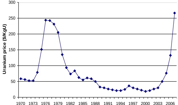
In particular, Figure 1(a) shows that from 1971 to 1973 uranium price has decreased from 59.15$/KgU to 52.39$/KgU. Then, it has considerably jumped to attain 243.29$/KgU in 1976. Although uranium price was still very high until 1979 (more than 200$/KgU), it has declined to 18.73$/KgU in 2000. By the beginning of 2000s (in particular from 2003) uranium price has started a smooth increase to reach 266.52 $/KgU in 2007.
Figure 1. (a) Uranium price
Figure 1(b) depicts the evolution of primary uranium production. It shows that by 1970, uranium production has gradually increased to reach a peak of about 69692 tU in 1980. Then, it has decreased to tumble down to 31503 tU in 1994. Since this date to 2007, production has increased but in a way which is largely less spectacular than the one observed in the mid-1970s.
12Million of dollars.
13International Atomic Energy Agency (IAEA).
0 50 100 150 200 250 300
1970 1973 1976 1979 1982 1985 1988 1991 1994 1997 2000 2003 2006
U
ra
n
iu
m
p
ri
c
e
($
/K
g
U
Figure 1. (b) Uranium production
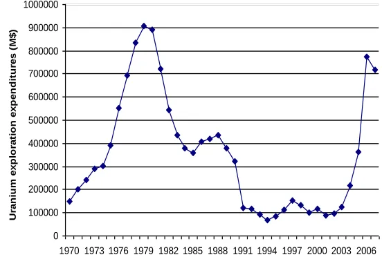
Figure 1(c) shows that uranium exploration expenditures evolution is very similar to the ones of uranium price and uranium production. Indeed, uranium exploration expenditures have started increasing in 1970 until reaching a peak of 907932 M$ in 1979. Then, from the beginning of 1980s, they have declined to 70325 M$ in 1994. In contrast, from the beginning of 2000s exploration expenditures have gradually increased again to reach a new peak of 773844 M$ in 2006.
Figure 1. (c) Uranium exploration expenditures
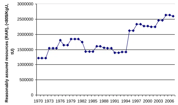
Finally, Figure 1(d) presents uranium reserves evolution. It is possible to distinguish three periods. The first one has started from the beginning of 1970s and lasted until the beginning of 1980s, during which the reserves have increased. The second one has started from the beginning of 1980s and lasted until the beginning of 1990s, during which the reserves have remained relatively constant. The third one has started from the beginning of 1990s and lasted until the end of the considered time period, during which uranium reserves have increased.
0 10000 20000 30000 40000 50000 60000 70000 80000
1970 1973 1976 1979 1982 1985 1988 1991 1994 1997 2000 2003 2006
U
ra
n
iu
m
p
ro
d
u
c
ti
o
n
(tU
)
0 100000 200000 300000 400000 500000 600000 700000 800000 900000 1000000
1970 1973 1976 1979 1982 1985 1988 1991 1994 1997 2000 2003 2006
U
ra
n
iu
m
e
x
p
lo
ra
ti
o
n
e
x
p
e
n
d
it
u
re
s
(
M
$
Figure 1. (d) Uranium reserves
These figures permit to show that there may be close relationships between uranium price, production, exploration expenditures and reserves since we can distinguish similar trends. In this sub-section, we limit our analysis to the above qualitative description of variables evolution. However, we analyse possible interactions and interdependence between these variables in section 3.2.3 when discussing the empirical results.
It is worthy to note that in our definition of uranium reserves, we consider the definition adopted by the OECD-NEA as reported in the Red Book Retrospective: Forty years of uranium resources, production and demand in perspective (OECD/NEA, 2006). According to this definition, uranium reserves refer to Reasonably Assured Resources (RAR)14 belonging to the cost category below 80$/KgU15. In fact,
reserves are in general defined as resources recoverable at a cost which is less than or equal to the upper cost limit of the lowest cost category. Therefore, the cost level that we consider for reserves definition is 80$/kgU for all the time period.
2.2 Empirical methodology
To investigate the effect of uranium price fluctuations on uranium production, exploration expenditures and reserves, we consider the following VAR(p) model:
14According to OECD/NEA (2006), RAR represent uranium that occurs in known mineral deposits of a given
size, grade and configuration that it could be recovered within the given production cost ranges, with currently proven mining and processing technology.
15Reserves discoveries follow the price development. In fact, the limit of the mineable ore is set by the point at
which the concentration falls to a level where mining is no longer economic at the contracted price. Therefore, a price rise is expected to generate new resources/reserves. These uranium resources are generally classified according to their degree of economic competitiveness, measured in terms of cost ranges (which depends on the contracted price level), and degree of confidence in resources estimations. Several classification systems exist. The NEA-IAEA is the most refered one. For a more comprehensive presentation of this classification system and some comparison with other ones, interested reader can look at OECD/NEA (2006). Also, Fujita and Silvennoinen (1985) present a brief discussion about the evolution of the NEA-IAEA classification system as well as the historical change in uranium resources.
0 500000 1000000 1500000 2000000 2500000 3000000
1970 1973 1976 1979 1982 1985 1988 1991 1994 1997 2000 2003 2006
R
e
a
s
o
n
a
b
ly
a
s
s
u
re
d
r
e
s
o
u
rc
e
s
(
R
A
R
),
(
<
8
0
$
/K
g
U
,
tU
t i t i p
i
t c y
y
1 =
=
(1)
where yt is a (41) vector of endogenous variables , c=(c1,...,c4) is the
1)
(4 intercept vector of the VAR, is the ith (44) matrix of autoregressive
coefficients for i=1,2,...,p, and t =(1t,...,4t) is the (41) generalisation of
innovation processes which represent unobservable zero-mean white noise processes with a time invariant positive-definite variance-covariance matrix.
The advantage of using VAR model is that it provides a multivariate framework where the changes in a particular variable are related to changes in its own lags and to changes in other model variables and the lags of those variables. The VAR model treats all variables as jointly endogenous and does not impose a prior restrictions on structural relationships. Because the VAR expresses the dependent variables in terms of predetermined lagged variables, it is a reduced-form model.
In this paper, we start by estimating a VAR model as it was defined by the equation (1) where all variables are expressed in natural logarithm. We call this VAR model the symmetric specification. Furthermore, on the basis of the previous empirical studies on oil price fluctuations effects on the economic activity, in particular on Mork (1989), we consider an asymmetric VAR model specification in which price increase and decrease are considered as a separate variables. More specifically, the asymmetric VAR model specification distinguishes between the positive changes in the uranium price (Pt), and the negative changes (Pt) as
follows:
otherwise P P if P P
Pt t t t t
0
0 >
= 1 1
and
otherwise P P if P P
Pt t t t t
0
0 <
= 1 1
where Pt being the natural logarithm of uranium prices. Figure 2 illustrates
annual uranium price changes from 1970 to 200716.
The advantage of the asymmetric specification is two fold. First, since it was largely admitted that the low uranium price level is an important limitation to the development of new production and exploration activities, that is, to discovering new reserves (Mays (2005); De Montessus (2008)), the asymmetric specification permits to show if uranium production, exploration expenditures and reserves are significantly influenced by price decrease. It also permits to show if there is any asymmetric reaction of production, exploration expenditures and reserves to price
16Each vertical bar in the graph represents the difference between price levels at time t and (t1).
variations, that is, to show if those variables are more sensitive to price increase rather than price decrease and vice-versa.
Figure 2. Uranium price variations from 1970 to 2007
In order to analyse the system's response to uranium price shock, the VAR system can be transformed into its Moving Average (MA) representation:
=0 1
=
i ti t
y
(2)
where 0 is the identity matrix and is the mean of the process
) ) (
=
( 1
0
= c
I i
i n
. The MA representation is used to obtain both the
impulse-response functions (IRFs) and the forecasting error variance decomposition (VD). In particular, while the IRFs permit to assess the dynamic impact of a one variable shock on the other system endogenous variables, the VD shows the proportion of the unanticipated changes of a variable that is explained by its own innovations and by shocks in other variables of the system.
In order to simulate IRFs, we examine the response of the system to 1% uranium price shock as well as to the orthogonal impulses by using the Cholesky decomposition. The response to orthogonal impulses assumes that shocks in different variables are independent and implies choosing an ordering for the system variables since this method of orthogonalisation involves the assignment of contemporaneous shocks only to specific series (Lütkepohl, 2006). Thus, the first variable in the ordering is not contemporaneously affected by shocks to the remaining variables, but shocks to the first variable affect the other variables in the system. By the same, a shock in the second variable affects contemporaneously the other variables (with the exception of the first one), but the second variable itself is not contemporaneously affected by a shock in one of them, and so on.
-100 -50 0 50 100 150
1970 1972 1974 1976 1978 1980 1982 1984 1986 1988 1990 1992 1994 1996 1998 2000 2002 2004 2006
Pr
ic
e
v
a
r
ia
ti
o
In this paper, we have assumed the following Cholesky ordering: uranium price, uranium production, uranium exploration expenditures and uranium reserves17.
Thus:
yt ={Pt,Yt,Expt,Rt} (4)
Using Cholesky decomposition, the innovations of current and past one-step ahead forecast errors are orthogonalised so that the resulting covariance matrix is diagonal. This assumes that in this pre-specified ordering, the uranium reserves react indirectly to uranium price fluctuations via the effect of uranium price on production and exploration expenditures. Uranium price variable is thus ranked as an exogenous variable which has an immediate impact on the uranium production and then uranium exploration expenditures which is, itself, allowed to feed changes in uranium reserves.
Before studying the effects of uranium price shocks, we proceed to investigate the stochastic proprieties of the time series considered in the VAR model by analysing their order of integration on the basis of unit root tests. We perform the Augmented Dickey and Fuller (1979, 1981) (ADF) and Phillips and Perron (1988) (PP) stationarity tests. If all variables are stationary in levels, i.e. I(0), VAR model specification in levels is appropriate. However, if variables have a problem of non-stationarity, the question of differencing series arises. According to Hamilton (1994), one option in such case is to ignore the non-stationarity altogether and simply estimate the VAR in level, relying on standard t and Fdistribution for testing
any hypothesis. In Hamilton's words, this strategy has three commendable features. “First, the parameters that describe the system's dynamics are estimated consistently. Second, even if the true model is a VAR in differences, certain functions of the parameters and hypotheses tests based on a VAR in levels have the same asymptotic distribution as would estimates based on differenced data. Third, a Bayesian motivation can be given for the usual t or Fdistributions
for test statistics even when the classical asymptotic theory for these statistics is non-standard” (Hamilton (1994), p. 652).
The alternative option is to difference any apparently non-stationary variable before estimating the VAR model. If the true process is a VAR in differences, then differencing should improve the small sample performance. The drawback of this approach is that when the true process may not be a VAR in differences. Some of the series may in fact have been stationary, or perhaps some linear combinations of the series are stationary, as in a cointegrated VAR. According to Sims (1980) and Hamilton (1994) in such circumstances defining a VAR in differenced form is mis-specified.
17Since variables ordering is crucial and can change the dynamics of the VAR system, and since
making the assumption that the uranium price is contemporaneously exogenous could be restrictive, we also consider, as robustness check, an alternative ordering namely: uranium
production, uranium price, uranium exploration expenditures and uranium reserves. Thus:
yt ={Yt,Pt,Expt,Rt} (3)
Table 1a. Results of ADF tests
Tests on levels18 Tests on first differences
ADF statistic
Critical value
Lag
number19 statistic ADF Critical value number Lag
t
P 0.42 -1.95 1 -2.05** 20 -1.95 0
t
P -1.81* -1.95 0 --- --- ---
t
P -3.28** -2.94 0 --- --- ---
t
Exp 0.21 -1.95 1 -3.74*** -1.95 0
t
R 1.24 -1.95 0 -5.95*** -1.95 0
t
Y 0.17 -1.95 1 -3.16*** -1.95 0
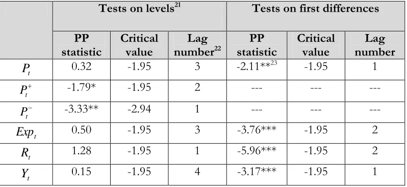
Table 1b. Results of PP tests
Tests on levels21 Tests on first differences
PP
statistic Critical value numberLag 22 statistic PP Critical value number Lag
t
P 0.32 -1.95 3 -2.11**23 -1.95 1
t
P -1.79* -1.95 2 --- --- ---
t
P -3.33** -2.94 1 --- --- ---
t
Exp 0.50 -1.95 3 -3.76*** -1.95 2
t
R 1.28 -1.95 1 -5.96*** -1.95 2
t
Y 0.15 -1.95 4 -3.17*** -1.95 1
18Note that for ADF stationarity test, the null hypothesis is that the variable has a unit root. When testing for the
stationarity, we consider specifications with constant and trend, only with constant and without constant and trend.
19To choose the optimal lag number, we are based on the autocorrelation functions. In fact, we retained a
maximum lag number which corresponds to the last lag number for which the autocorrelation function is statistically significant. Then, starting from this maximum lag number, we choose the lag number that minimizes AIC and SC information criteria.
20***significant at 1%, **significant at 5%, *significant at 10%.
21Note that for PP stationarity test, the null hypothesis is that the variable has a unit root. When testing for the
stationarity, we consider specifications with constant and trend, only with constant and without constant and trend.
22To choose the optimal lag number, we are based on the autocorrelation functions. In fact, we retained a
maximum lag number which corresponds to the last lag number for which the autocorrelation function is statistically significant. Then, starting from this maximum lag number, we choose the lag number that minimizes AIC and SC information criteria.
Table 2a. Results of cointegration test: symmetric case
Number of CR24/Trace
statistic and CV25 Trace Statistic
26 CV at 5% CV at
1%
3
r 2.15 12.25 16.26
2
r 9.35 25.32 30.45
1
r 29.55 42.44 48.45
0 =
r 54.86 62.99 70.05
Table 2b. Results of cointegration test: asymmetric case
Number of CR27/Trace
statistic and CV28 Trace Statistic
29 CV at 5% CV at
1%
2
r 3.49 25.32 30.45
1
r 9.97 42.44 48.45
0 =
r 30.70 62.99 70.05
Subsequently, the other area of debate is whether an unrestricted VAR should be used when the variables in the VAR are cointegrated. There is a body of literature that supports the use of a vector error correction model (VECM), or cointegrating VAR, in this case. Nevertheless, it has been argued that in the short-term, unrestricted VAR performs better than a cointegrated VAR or VECM. For instance, Naka and Tufte (1997) demonstrated the advantages of unrestricted VAR by examining IRFs in cointegrated systems. According to their analysis, a system of cointegrated variables is estimated either as a VAR in levels or as a VECM model, where the latter is a restricted version of the former. If there is cointegration, imposing this restriction will yield more efficient estimates. However, in the short-run, VEC estimates are less accurate than those from a VAR. Their Monte Carlo analysis shows that the loss of efficiency from VAR estimation is not critical for the commonly used short-run. In addition Naka and Tufte (1997), other researchers like Engle and Yoo (1987), Clements and Hendry (1995), and Hoffman and Rasche (1996) showed that an unrestricted VAR is superior (in terms of forecast variance) to a restricted VEC model in the short-run when the restriction is true.
The results of stationarity tests are presented in Tables 1a and 1b. They show that all variables are stationary on the first differences, except Pt and Pt which are
stationary on level. On the basis of the mentioned debates of the advantages and drawbacks of different VAR model specifications, and considering the possibility of the existence of cointegration relationships between the integrated variables, we test for the presence of cointegration relationships by using Johansen cointegration test
24Denotes cointegration relationships. 25Denotes critical values.
26Here, we report the results of the test after including linear trend in cointegration relationship. Even when
including a constant results are still the same.
27Denotes cointegration relationships. 28Denotes critical values.
29Here, we report the results of the test after including linear trend in cointegration relationship. Even when
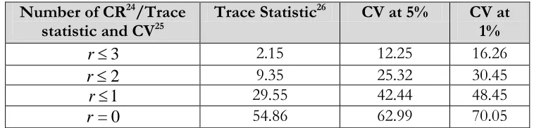
(Johansen (1991); Johansen (1995)). Results, based on trace statistics at 1% and 5% significance levels, are presented in Tables 2a and 2b. They show that there is no evidence of cointegration relationships between the integrated variables. As a consequence, we define the vector yt in equation (1) to be given by the first
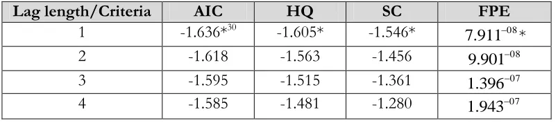
differences of the variables. To determine the optimal lag length of the symmetric and asymmetric VAR model specifications, we make use of Akaike (AIC), Hannan-Quinn (HQ), Schwarz (SC) and Forcasting Prevision Error (FPE) criteria. The results are presented in Tables 3a and 3b. They show that for the symmetric VAR model, the optimal lag length is equal to 1. For the asymmetric VAR model, results of HQ and SC criteria show that the optimal lag length is equal to 1, whereas the results of AIC and EPE criteria show that it is equal to 2. Since we have a limited number of observations, we consider that the optimal lag length for the asymmetric VAR model specification is equal to 1.
Table 3a. VAR optimal lag number selection: symmetric case
Lag length/Criteria AIC HQ SC FPE
1 -1.636*30 -1.605* -1.546* 08
7.911 *
2 -1.618 -1.563 -1.456 08
9.901
3 -1.595 -1.515 -1.361 07
1.396
4 -1.585 -1.481 -1.280 07
1.943
Table 3b. VAR optimal lag number selection: asymmetric case
Lag length/Criteria AIC HQ SC FPE
1 -1.812 -1.351* -0.478* 0.166
2 -1.907*31 -1.063 0.536 0.165*
3 -1.575 -0.348 1.979 0.298
4 -1.532 -0.195 2.045 0.328
3.EMPIRICAL RESULTS
In this section, we present and discuss empirical results. In particular, we analyse in subsection 3.1 the results of Granger (1969)-causality tests. We turn in subsection 3.2 to the examination of the effects of uranium price shocks on production, exploration expenditures and reserves: first we present the results of the IRFs simulation (subsection 3.2.1), second we present the results of VD (subsection 3.2.2), and finally we discuss empirical findings in subsection 3.2.3.
3.1 Testing for Granger-causality
To investigate the structure of causality relationships between uranium price and other VAR model variables, we perform Granger (1969) causality test32. Results are
detailed in Tables 4a and 4b. Figure 3 depicts the structure -or direction- of causality relationships for the symmetric VAR model specification.
Table 4a. Results of Granger-causality test: symmetric case
Null hypothesis F-statistic Probability
t
Y does not Granger cause Pt 0.251 0.619
t
P does not Granger cause Yt 7.607 0.009***
33
t
Exp does not Granger cause Pt 0.370 0.547
t
P does not Granger cause Expt 9.725 0.003***
t
R does not Granger cause Pt 2.937 0.095*
t
P does not Granger cause Rt 1.287 0.264
t
Exp does not Granger cause Yt 3.545 0.068*
t
Y does not Granger cause Expt 2.627 0.114
t
R does not Granger cause Yt 0.227 0.636
t
Y does not Granger cause Rt 0.576 0.453
t
R does not Granger cause Expt 0.205 0.653
t
Exp does not Granger cause R 0.314 0.578
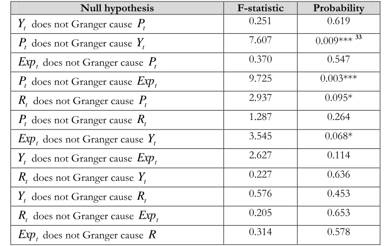
For the symmetric case (Cf. Table 4a) results show that the causality between uranium price and uranium production as well as between uranium price and uranium exploration expenditures is statistically significant. More specifically, they show that the causality relationship goes from uranium price to exploration expenditures as well as from uranium price to production. Results also show that the causality relationship between production and exploration expenditures is significant but going in one direction from exploration expenditures to production. As for the relationships between uranium reserves and other model variables, results show that there is no evidence of causal relationship going from uranium price to uranium reserves. However, the inverse is true: reserves cause uranium price. This may refer to Hotelling (1931) rule according to which the reserves level (or the extraction rate) determines the price of the (exhaustible) resource34. Further, results
show that, both, uranium exploration expenditures and uranium production do not Granger cause uranium reserves contrasting the intuition according to which uranium production and uranium exploration expenditures may represent the transmission channels through which uranium price affects uranium reserves.
32We use the same number of lags as in VAR model specifications. 33***significant at 1%, **significant at 5%, *significant at 10%.
34According to the Hotelling (1931) rule, the optimal use of an exhaustible resource implies that the resource
Figure 3. Granger-causality relationships structure: symmetric case.
Table 4b. Results of Granger-causality test: asymmetric case
Null hypothesis F-statistic Probability
t
Y does not Granger cause Pt 0.169 0.682
t
P does not Granger cause Yt 4.103 0.050** 35
t
Exp does not Granger cause Pt 1.270 0.267
t
P does not Granger cause Expt 4.468 0.042**
t
R does not Granger cause Pt 2.252 0.142
t
P does not Granger cause Rt 0.020 0.886
t
Y does not Granger cause Pt 0.247 0.622
t
P does not Granger cause Yt 0.238 0.628
t
Exp does not Granger cause Pt 0.805 0.376
t
P does not Granger cause Expt 0.028 0.867
t
R does not Granger cause Pt 0.234 0.631
t
P does not Granger cause Rt 0.652 0.424
t
Exp does not Granger cause Yt 3.545 0.068*
t
Y does not Granger cause Expt 2.627 0.114
t
R does not Granger cause Yt 0.227 0.636
t
Y does not Granger cause Rt 0.576 0.453
t
R does not Granger cause Expt 0.205 0.653
t
Exp does not Granger cause R 0.314 0.578
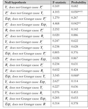
The results of the Granger-causality tests of the asymmetric specification (Cf. Table 4b) corroborate those ones corresponding to the symmetric specification. In fact, they show that positive uranium price shock (Pt) significantly causes uranium
production as well as uranium exploration expenditures and that the uranium exploration expenditures significantly cause the uranium production. Also, results show that, as in the symmetric VAR specification, no significant causal relationship can be indentified from uranium production to uranium reserves or from uranium exploration expenditures to uranium reserves. Further, no significant causal relationship can be identified between uranium reserves and uranium prices neither in one direction nor in the other.
Finally, the results of the asymmetric specification show that there is no significant causal relationships between negative uranium price shock (Pt) and the
other variables. This result gives a first evidence that the effect of price increase, i.e. positive price shock, is more felt than the effect of price decrease, i.e. negative price shock.
In sum, the results of Granger-causality tests of the symmetric and asymmetric VAR model specifications permit to identify that while uranium price does not cause the uranium reserves, it significantly causes the uranium production as well as the uranium exploration expenditures, and that there is some evidence of asymmetric reaction of the uranium production and exploration expenditures to price fluctuations since uranium production and exploration expenditures significantly react to a positive price shock but not to a negative one.
3.2 Impacts of uranium price shocks on uranium reserves
In this subsection, we assess the effect of uranium price fluctuations on uranium production, exploration expenditures and reserves. After estimating the symmetric and asymmetric VAR models (Cf. Tables A.1 and A.2 in Appendix A), we present under subsection 3.2.1, the results of IRFs. Then, in subsection 3.2.2, we analyse the sources of variation of each variable by using the VD. Finally, we discuss those results in subsection 3.2.3.
3.2.1 Impulse response functions analysis
The graphic representation of IRFs traces the effects of a one-time shock to one of the innovations on current and future values of the endogenous variables. IRFs for symmetric and asymmetric VAR model specifications are depicted in Figures. 4(a), 4(b), 5(a), 5(b) and 636. We also report the results of elasticities of the model
variables to uranium price shock in Tables 5(a) and 5(b)37.
According to Runkle (1987), reporting IRFs without standard error bars is equivalent to reporting regression coefficients without t-statistics. Therefore, as an indication of significance, IRFs figures are reported with bootstrap/Monte Carlo two-standard error bounds. In each IRFs figure, the middle continuous line
36IRFs that we report represent the response of the system to 1% uranium price shock as well as to the
orthogonal impulses.
37Since the results show that a negative uranium price shock ( )
t
represents the IRF while the broken lines represent confidence intervals. When the horizontal line falls into the confidence interval (for all time periods or for only some particular time periods), the null hypothesis that there is no effect of uranium price shock on the other model variables cannot be rejected, that is, there is evidence of statistical non significance.
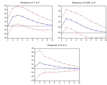
Figure 4a displays the orthogonalised IRFs to a one standard deviation uranium price innovation for the symmetric VAR specification. It shows that the uranium price shock engenders a significant increase in uranium production as well as in uranium exploration expenditures. This result goes the same way as the results of the estimation of the symmetric VAR model (Cf. Table A.1 in the Appendix A) showing that the uranium price is significantly correlated with uranium production and exploration expenditures. IRFs in Figure 4(a) mainly show that the uranium production start rising at the first year after the shock and reach a peak at the third year after the shock to start decreasing after that. Thus, when uranium price increases, uranium producers being tempted by the possibility to make new profits will increase their production. The reaction of the production to the price shock becomes statistically significant with a time lag of one year, and it is still significant untill the fourth year after the price shock. After that, the production reaction progressively dissipates implying that such reaction is transitory.
Figure 4. (a) Orthogonalised IRFs to a one standard deviation uranium price innovation for the symmetric VAR specification
-.03 -.02 -.01 .00 .01 .02 .03 .04 .05
1 2 3 4 5 6 7 8 9 10
Response of Y to P
-.05 .00 .05 .10 .15 .20 .25
1 2 3 4 5 6 7 8 9 10
Response of EXPL to P
-.03 -.02 -.01 .00 .01 .02 .03 .04 .05
1 2 3 4 5 6 7 8 9 10
Figure 4(b) and Table 5a, presenting the reaction of uranium production to 1% price increase, show that uranium production elasticity to 1% uranium price shock goes from 0.09% two years after the shock to 0.11% three years after the shock and that it is statistically non significant the first year after the shock. This corroborates the results of the orthogonalised IRFs according to which the reaction of production to price increase is not instantaneous. In this context, historical analysis of the uranium price-prodution relationship shows that in the beginning of 1970s, the uranium production increase has started in 1975, two or three years lag after the uranium price increase in 1973 (OECD/NEA, 2006). From the fifth year after the shock, the production reaction (elasticity) becomes statistically non significant implying that the price shock effect is not sustainable.
On the other hand, IRFs show that uranium price shock engenders an instantaneous and significan t increase in exploration expenditures (Cf. Figure 4(a)). This effect lasted from the first year of the shock untill the fourth year after the shock. This result confirms the conclusions of Greenwood (1981), Price (1984), Harris DeVerle (1984), Underhill (1990), Price (2005) and OECD/NEA (2006) which assert that it exists a causal relationship between uranium price and exploration expenditures. In fact, when the uranium price increases the production increases which may engender a need for expanding exploration activities and discovering new resources. Figure 4(b) and Table 5a show that the uranium exploration expenditures elasticity to price shock is equal to 0.62% two years after the shock. It decreases then to reach 0.29% five years after the shock. After the fifth year, it becomes statistically non significant.
Figure 4. (b) 1% uranium price shock IRFs for the symmetric VAR specification.
-.05
.00 .05 .10 .15 .20 .25
1 2 3 4 5 6 7 8 9 10
Response of Y to P
-0.2 0.0 0.2 0.4 0.6 0.8 1.0
1 2 3 4 5 6 7 8 9 10
Response of EXPL to P
-.08 -.04 .00 .04 .08 .12 .16 .20 .24
1 2 3 4 5 6 7 8 9 10
The IRF displaying uranium reserves reaction to uranium price shock suggests that uranium reserves positively react to uranium price shock. However, the reaction is not statistically significant. Estimation of the symmetric VAR model as shown in Table A.1 in Appendix A also shows that there is no significant correlation between uranium price and uranium reserves. Although this result may, at a first glance, seem surprising, it corroborates results of OECD/NEA (2006) which argues that although uranium price is expected to indirectly affect resources because it affects exploration expenditures and production, the relationship between uranium price and uranium reserves is seldom readily obvious. One reason for this, is the existence of time lag between exploration activities, effective discoveries and reporting of new discovered reserves. Thus, although price increase may induce production increase which may feed in exploration expenditures, the effect of exploration expenditures on adding to the reserves base can only be perceived in the long-run.
To sum up, the IRFs results of the symmetric VAR specification show that both uranium production and uranium exploration expenditures respond significantly and positively to uranium price shock. However, uranium reserves reaction which is positive, is statistically non significant along the whole time period.
Figure 5. (a) Orthogonalised IRFs to a one standard deviation uranium price
innovation for the asymmetric VAR specification: positive price shock (Pt)
-.02 -.01 .00 .01 .02 .03 .04 .05
1 2 3 4 5 6 7 8 9 10
Response of Y to P+
-.05 .00 .05 .10 .15 .20 .25
1 2 3 4 5 6 7 8 9 10
Response of EXPL to P+
-.04 -.03 -.02 -.01 .00 .01 .02 .03 .04 .05
1 2 3 4 5 6 7 8 9 10
Figure 5. (b) 1% uranium price shock IRFs for the asymmetric VAR specification: positive price shock (Pt).
When considering the asymmetric VAR model (the results of estimating this model are presented in Table A.2 in Appendix A, Figure 5(a), depicting the effect of positive uranium price shock (Pt), shows that the response of uranium production
is positive and statistically significant at 10%. The reaction of exploration expenditures is also positive and statistically significant corroborating the IRFs results relative to the symmetric VAR model specification. The exploration expenditures reaction stops to be significant from the third year following the shock. In particular, Figure 5(b) and Table 5b show that uranium exploration expenditures elasticity goes from 0.08% the second year after the shock to 0.05% the third year. On the other hand, the reaction of uranium reserves to a positive uranium price shock is also statistically non significant as in the symmetric VAR model specification (uranium reserves slightly increase by the end of the first year after the shock to peak at the third year and decrease then until the end of the time period). In this context, the results of estimating the asymmetric VAR model (Cf. Table A.2 in Appendix A) show that there is no significant correlation between uranium price increase and uranium reserves.
Finally, Figure 6 which depicts IRFs relative to a negative uranium price shock
)
(Pt , shows that the reactions of the production, exploration expenditures as well
as reserves are statistically non significant although they are correctly signed, i.e. they decrease after a negative price shock. This may refer to the lack of competitiveness of the uranium market and reflect the fact that the uranium price, production, exploration and reserves are not always governed by the supply-demand rules as for
-.01 .00 .01 .02 .03 .04
1 2 3 4 5 6 7 8 9 10
Response of Y to P+
-.04 .00 .04 .08 .12 .16
1 2 3 4 5 6 7 8 9 10
Response of EXPL to P+
-.03 -.02 -.01 .00 .01 .02 .03
1 2 3 4 5 6 7 8 9 10
any traditionnal commodity but also governments intervention and other political issues38.
Table 5a. Elasticity of variables to uranium price shock: symmetric case
Period
t
Y Expt Rt
2 0.092 (0.047)39 0.628(0.177) 0.078(0.076)
3 0.113(0.044) 0.478(0.168) 0.038 (0.042) 4 0.101(0.046) 0.414(0.186) 0.038(0.037) 5 0.079(0.046) 0.298(0.188) 0.025(0.031) 6 0.057(0.043) 0.209(0.179) 0.017(0.025)
Table 5b. Elasticity of variables to uranium price shock: asymmetric case
Period
t
Y Expt Rt
2 0.011(0.006)40 0.081(0.035) -0.000(0.014)
3 0.013(0.007) 0.056(0.030) 0.002(0.006) 4 0.011(0.007) 0.044(0.029) 0.002(0.004) 5 0.008(0.006) 0.029(0.025) 0.001(0.003) 6 0.005(0.005) 0.019(0.021) 0.001(0.002)
Figure 6. Orthogonalised IRFs to a one standard deviation uranium price
innovation for the asymmetric VAR model specification: negative price shock (Pt).
38According to the OECD/NEA (2006) “while the uranium market price is now largely controlled by the perception of the
balance between supply and demand, this has not always been the case. Prior to the end of the Cold War, military demand acted
to distort the treatment of uranium as a commodity due to national security requirements and secrecy”.
39Values between brackets denote the standard error (bootstrap/Monte Carlo). 40Values between brackets denote the standard error (bootstrap/Monte Carlo).
-.05 -.04 -.03 -.02 -.01 .00 .01 .02
1 2 3 4 5 6 7 8 9 10 Response of Y to
P--.16 -.12 -.08 -.04 .00 .04 .08
1 2 3 4 5 6 7 8 9 10 Response of EXPL to
P--.06 -.05 -.04 -.03 -.02 -.01 .00 .01 .02 .03
P-Thus, results of analyzing the effects of uranium price fluctuations on uranium production, exploration expenditures and reserves show that no significant causal relationship between uranium price and uranium reserves can be identified. Nevertheless, in the symmetric VAR specification, the reaction of uranium production and uranium exploration expenditures, already defined as transmission channels through which it was expected that uranium price fluctuations will affect reserves, is statistically significant. In the asymmetric VAR specification, when there is a positive uranium price shock (Pt), the reaction of exploration expenditures and production are still statistically significant41. When there is negative uranium price
shock (Pt), reaction of all variables is statistically non significant pointing out,
therefore, the asymmetric reaction of exploration expenditures and, to a lesser extent, the uranium production to uranium price variations42.
3.2.2 Variance decomposition analysis
By using IRFs, we have illustrated the qualitative response of variables to uranium price shock. We now examine the forecasting error variance decomposition (VD) to determine the proportion of variables variations which is engendred by shocks in variables themselves as opposed to shocks in other variables.
Tables 6a and 6b present the VD analysis for the symmetric and asymmetric VAR model specifications43.
Table 6a. Variance decomposition: symmetric case
Year/Variable
t
P Yt Expt Rt
Yt
1 0.001 99.998 0.000 0.000
2 9.722 89.340 0.891 0.045
3 20.114 77.589 1.408 0.888
4 26.565 70.148 1.667 1.618
5 29.896 66.241 1.782 2.079
Expt
1 6.685 7.623 85.691 0.000
2 26.110 14.795 58.486 0.607
3 35.374 12.463 50.144 2.017
4 40.404 11.285 45.623 2.686
5 42.611 10.768 43.531 3.087
Rt
1 0.301 5.757 8.893 85.047
2 2.333 5.976 9.469 82.219
3 3.283 5.879 9.717 81.119
4 3.937 5.836 9.647 80.578
5 4.246 5.822 9.631 80.299
41At 10% significance level for uranium production.
42To check the robustness of these conclusions, we simulate IRFs with alternative variables ordering as
described in section 2.2. The results are still the same as in the pre-specified variables ordering. These IRFs figures are available upon request.
The results of the symmetric VAR model specification (Cf. Table 6a) show that in the first year following uranium price shock, the production variation is mainly explained by its past innovations, i.e. 99.9%. Uranium price fluctuations seem to play only very marginal role in explaining production variations, i.e. 0.1%. Nevertheless, in the second year after the shock, while uranium price shock explains 9.7% of production variations, the exploration expenditures explain 8.9%. The role of uranium price fluctuations in explaining prodution innovations continue to increase going from 9.7% in the second year after the shock to 29.89% in the fifth year. However, the role of exploration expenditures fluctuations decreases to 1.78% in the fifth year after the shock. Therefore, the role of exploration expenditures fluctuations in explaining production variations is still largely less important than the role of uranium price shock. The role of reserves is also minor since their contribution to production variations does not go beyond 4.5% the first year after the shock and 2.07% the fifth year.
The uranium price fluctuations also significantly contribute to explaining exploration expenditures variations. In the second year after the price shock, their contribution reach 26.11%. For the same year, the remaining of exploration expenditures variations is mainly explained by its own innovations, i.e. 58.48%, and by production fluctuations, i.e. 14.79%. Five years after the price shock, price fluctuations explain 42.61% of uranium explorations expenditures variations. This result confirms once again the existence of a close correlation between uranium price and exploration expenditures. For the same year, the production fluctuations explain 10.76% of the exploration expenditures variations.
Table 6b. Variance decomposition: asymmetric case
Year/Variable
t
P Pt Yt Expt Rt
Yt
1 1.252 11.042 87.705 0.000 0.000 2 9.449 9.306 78.186 2.933 0.123 3 16.121 8.387 70.897 4.041 0.551 4 19.703 7.894 66.817 4.737 0.847 5 21.389 7.667 64.901 5.031 1.009
Expt
1 8.675 2.788 7.461 81.073 0.000 2 22.233 3.209 13.871 59.663 1.022 3 27.805 2.848 12.880 55.013 1.452 4 30.479 2.721 12.348 52.735 1.715 5 31.583 2.657 12.067 51.855 1.835
Rt
The past innovations of uranium reserves explain 85.04% of reserves variations in the first year after the price shock, 82.21% in the second year, and 81.11% in the third year. The role of uranium price fluctuations in explaining reserves variations is very low going from 0.3% in the first year after the shock to 4.24% in the fifth year. Uranium exploration expenditures and uranium production variations explain 5.87% and 9.71% respectively of the reserves variations in the third year after the shock.
In sum, VD results of the symmetric VAR model specification show that uranium price shock plays significant role in explaining uranium production and explorations expenditures innovations, especially in the long-run. However, it marginally contributes to explaining uranium reserves variations.
The VD results of the asymmetric VAR model specifications are presented in Table 6b. They give evidence of the asymmetric aspect in the reaction of uranium production and uranium exploration expenditures to price shock. In fact, with regard to the uranium production variations, while a positive price shock plays a gradually increasing role in explaining the uranium production variations, i.e. from 1.25% in the first year after the shock to 21.38% in the fifth year, a negative uranium price shock plays a gradually decreasing and less important role in explaining the uranium production: from 11.04% in the first year after the shock to 7.66% in the fifth year. Therefore, the role of a negative uranium price is steadily decreasing to the profit of the role of positive price shock and exploration expenditures. The contribution of the latter variable variations is growing going from 2.93% in the second year after a negative price shock to 5.03% in the fifth year.
The same holds when looking at the VD of uranium exploration expenditures. In fact, the positive uranium price shock explains the major variations of exploration expenditures, after its own innovations and before uranium production variations, i.e. from 8.67% in the first year after the shock to 31.58% in the fifth year after the shock. However, the negative variations of uranium price explain less than 3% of the explorations expenditures variations along the first five years.
When analysing the source of variations of uranium reserves, the results are almost similar to the ones relative to the symmetric VAR specification. In fact, uranium reserves variations are mainly explained by their own innovations, uranium explorations expenditures and uranium production. The uranium price fluctuations play a minor role in explaining reserves variations. This role does not go beyond 4.2% on average in the case of positive uranium price shock and 2.7% on average in the case of a negative uranium price shock. In contrast, uranium exploration expenditures and production respectively explain around 13% and 7.5% of reserves variations. Thus, once again the results of VD point out the fact that uranium price does not play a crucial role in explaining uranium reserves behaviour, corroborating therefore the IRFs result according to which there is no significant correlation between uranium price and uranium reserves.
3.2.3 Results discussion
expenditures relationship, and the third one deals with the uranium price-uranium reserves relationship. Below, these results are discussed.
Uranium price-uranium production relationship
The results of the symmetric and asymmetric VAR model specifications shows that uranium price increase exerts a significant effect on the uranium production. Also, the VD analysis points out the fact that a large part of the uranium production variation after price increase is explained by the price fluctuations44.
Figure 7, which shows the historical evolution of uranium price and uranium production from 1970 to 2007, corroborates the fact that it exists a close relationship between uranium price and uranium production since trends are similar although the timing of production data breakpoints have been produced with a certain time lag (as indicated by the IRFs results in section 3.2.1).
Figure 7. Uranium price vs uranium production
Such lag can be explained by the transaction process on the uranium market based on long-term contracts. For example, after the sharp uranium price decline by the end of 1970s, the production was still high during seven years after the price decline due to the fact that uranium producers operate on the market via long-term contracts which were contracted at a price level situated above the falling prices. Thus, these contracts have acted to sustain the production increase after price jump in the mid-1970s, although prices have declined few years after. Once these long-term contracts have been run out, the production has decreased again following the uranium price decrease45. The next long time period of falling prices during the
44The asymmetric Granger causality tests also show that a positive price shock significantly causes the
production.
45Note that the transaction on the uranium market relying on long-term contracts procedure may also explains
why uranium production does not significantly react to price decrease as shown by the results of the asymmetric analysis.
0 50 100 150 200 250 300
1970 1973 1976 1979 1982 1985 1988 1991 1994 1997 2000 2003 2006
U
ra
ni
um
pri
c
e
(
$
/K
gU
)
0 10000 20000 30000 40000 50000 60000 70000 80000
U
ra
ni
um
prod
uc
ti
on
(
tU
)
Uranium price