Learning a Transferable World Model by Reinforcement Agent
in Deterministic Observable Grid-World Environments
Jurgita Kapoit-Dzikien, Gailius Raškinis
Vytautas Magnus University Vileikos 8, LT-44404 Kaunas, Lithuania
e-mail: [email protected], [email protected]
http://dx.doi.org/10.5755/j01.itc.41.4.915
Abstract. Reinforcement-based agents have difficulties in transferring their acquired knowledge into new different environments due to the common identities-based percept representation and the lack of appropriate generalization capabilities. In this paper, the problem of knowledge transferability is addressed by proposing an agent dotted with decision tree induction and constructive induction capabilities and relying on decomposable properties-based percept representation. The agent starts without any prior knowledge of its environment and of the effects of its actions. It learns a world model (the set of decision trees) that corresponds to the set of explicit action definitions predicting action effects in terms of agent’s percepts. Agent’s planning component uses predictions of the world model to chain actions via a breadth-first search. The proposed agent was compared to the Q-learning and Adaptive Dynamic Programming based agents and demonstrated better ability to achieve goals in static observable deterministic grid-world environments different from those in which it has learnt its grid-world model.
Keywords: Adaptive agent; reinforcement learning; percept generalization; world model.
1. Introduction
Imagine a rat running in search for a food in lots of different mazes. An experimenter in animal cognition would be surprised to observe the rat perfectly navigating in one of the mazes but hitting walls and obstacles in the others. Otherwise stated, it seems that rats like other animals learn the effects of their basic actions in a way that is independent of their environ-ment.
Imagine a comparable situation of an adaptive agent placed in an artificial grid-world environment. Every cell of a grid is labeled with some symbol. The agent can perform a few basic actions. If it goes left, the contents of all cells shift right (imitating the movement of its “view of sight”). If it goes up, cell
contents shift down and so on1. The agent starts
without any knowledge of its environment and of the effects of its own actions. Having operated in one environment for some time the agent is transferred to some another. This new environment has a completely different rearrangement of cell labels (assuming that labels retain their meanings). Do the regularities learned by the agent in the first environment have any
1 This environment is not subject to the perceptual reference frame
assumption which requires that agent actions change only a small part of the agent’s perceptual input, the remaining steady input providing a background or frame.
sense in this second one? Should the agent continue learning or should it “reboot” and start learning from zero again?
Though adaptive agents are often thought as computational models of biological intelligence, these questions would be hard to many of them. In many agent designs, the knowledge learnt by an adaptive agent must be invalidated when the agent is confronted to a different environment (or even a different goal in the same environment) than that in which it has been learning. The transferability of learned knowledge to different environments is an important aspect of adaptive behavior. This aspect seemed to be underemphasized in the reinforcement learning research until very recently.
To address this challenge we have developed an
adaptive agent called LEAD12 that is able to operate in
a static observable deterministic grid-world environment roughly described above. The agent learns explicit action definitions in terms of its percepts and can predict the effects of its actions. This type of knowledge can be transferred and augmented in new environments that are different from those in which it has learnt its first experience.
2. Related work
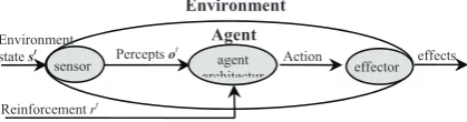
An adaptive agent is the system that perceives and acts upon its environment and improves its performance by adjusting its internal configurations and actions in response to feedback from its environment. Figure 1 illustrates the agent-environment interaction. The agent starts without any knowledge of its environment and of the effects of its
own actions. At every discrete time step t it receives
percept information ot through its sensors, processes
this information, e. g. updates its internal world
model, and selects some action at to be performed
through its effectors. The action typically alters the
state of the environment st+1 resulting in new percepts
ot+1 and a new percept-action cycle begins (Figure 1).
Figure 1. Illustration of an agent embedded into its environment
If agent’s percepts are representing the complete
environment state (e. g. ot { st), the environment is
called observable. If the environment state is changed solely by the agent’s actions, the environment is called static. If the same action performed in the same environment state but at two distinct time instants always results in the identical successor states, the environment is called deterministic. Otherwise the environment is called partially observable, dynamic and stochastic, respectively.
There are different agent architectures capable of associating agent’s percepts to its actions. Detailed descriptions of many complete agent architectures can be found in A Survey of Cognitive and Agent Architectures [1]. We are mostly interested by the agents that learn some knowledge body from their experience and by the aspect of transferability of that knowledge.
First, agents are provided their goals in different ways. The most widespread approach is that of reinforcement [11] [12] [14]. It assumes that there exists a dedicated reinforcement channel into an agent (Figure 1). Reinforcement values coming through this channel tell the agent which environmental states are preferred to the others, thus indirectly describing its goal. Another approach is to assume the existence of a dedicated “goal channel” through which agent’s goals
are directly “injected”3 into the system [10]. There are
other more biologically inspired approaches where an agent is supposed to have motivations, innate behaviors or to be able to extract reinforcement values from the ordinary sensory input [3] [16].
3 In humans, this would correspond to having mystical experiences
such as unexplained visions and desires.
Second, agents make different architectural assumptions about their percepts. The most common
assumption is to take percepts ot as an atomic state
identity label [15]. An alternative approach is to assume that perceptual information is decomposable and/or structured. In this latter case, percepts may be represented by a set of properties [5] [13] [16], described in propositional or the first-order logic [10]. The generalization capabilities of an agent have sense only if decomposable percept representation is used.
One of the most important dividing lines among agent architectures is the presence or absence of a world model. A world model is defined as a body of knowledge that tells the agent what are the expected outcomes of its actions in terms of its future percepts. The presence of a world model has clear architectural implications as only the world model makes an agent capable of planning, i. e. chaining sequences of its actions. We would distinguish three types of agent architectures: agents that learn utility values associa-ted to percepts or the percept-action pairs (model-free agents), agents that learn both utility values and a world model (model-based agents) and agents that learn only a world model (model-rich agents).
An example of a model-free method is Q-learning [15]. The Q-learning based agent selects its actions on the basis of the percept-action utility values (Q-values). It improves its performance in terms of cumulative positive reinforcement. However the table of Q-values is a type of knowledge that bounds the agent to pursue a single goal in the same environment. Some extensions to Q-learning such as function
approximation [2] and relational reinforcement
learning [6] [7] aim to abstract from specific goals pursued and to exploit the results of previous learning phases in new situations. Function approximation approach uses properties-based percept represen-tation [2] [7]. It generalizes over properties in order to approximate the Q-function. Relational reinforcement represents percepts as a set of ground facts stated in the first order logics [6]. It combines Q-learning and supervised learning by learning Q-function with relational regression tree algorithm [4]. These extensions to Q-learning make computationally intrac-table learning problems tracintrac-table, and increase the transferability of learned knowledge. However they do not compensate for the fact that an agent still lacks a world model and explicit definitions of its actions.
Examples of model-based architectures are Dyna
[11], TD(O) [12], and ADP [9]. Model-based agents
also rely on the identity-based percept representation. Besides percept utility values they learn a world model consisting of a set of conditional transition probabilities of percept identities p(ot+1|ot,at). Model-based agents, like model-free agents, select their actions on the basis of percept utility values. Thus, the probabilistic world model is seen not as a means for constructing explicit action plans but as a body of knowledge useful to the convergence of percept utility values to the optimal policy. Though model-based
Perceptsot
Environment
Agent
effector
sensor Action effects
Reinforcement rt Environment statest
agents would be able to adapt to changing goals in the same environment, they would not be capable to predict the effects of their actions in new environ-ments.
Among examples of model-rich agents are LIVE [10], the architecture proposed by Drescher [5], SRS/E [16], and CALM [13]. Model-rich agents learn their world model for the purpose of planning action sequences. Except for LIVE, model-rich agents rarely learn explicit action definitions. The world model of a model-rich agent often consists of the set of
accumulated elementary experiences of the type <ot,
at, ot+1>. Model-rich agents use properties-based
percept representation. Thus, part of the world-model experiences can be generalized by omitting (e. g.
replacing by a wildcard) some properties within ot,at,
orot+1 components. This capability of generalization is
enough for pursuing different goals in the same environment, but not enough to solve the grid-world task outlined in the introductory section. On the other hand, SRS/E and CALM are advanced agent architectures in other respects. SRS/E can operate in stochastic environments, while CALM is designed to operate in deterministic but partially observable environments.
LIVE is model-rich agent that learns explicit action descriptions. It represents its percepts as a set of ground facts stated in the language of the first order
logics4. States are generalized into a set of the
action-defining STRIPS-like first-order logic rules. However, the LIVE approach relies on the perceptual frame hypothesis, which is not satisfied in the grid-world challenge outlined in the introductory section.
3. LEAD1 architecture
The underlying hypothesis of our approach is that the transferability of knowledge is intrinsically related to the generalization capabilities of an agent. An agent must learn to predict outcomes of its actions (a world model) on the basis of its percepts in such a way that regularities/laws establishing prediction hold for different unseen environments. This can be achieved only if decomposable percept representation is used and the agent is capable of extracting relevant properties and abstracting from irrelevant properties at the same time.
This kind of reasoning has driven us to design the
LEAD1 agent. The life of the agent is organized in
epochs each epoch consisting of a number of discrete time steps until it reaches the goal state. Agent
recognizes that a goal state is reached at time t if it
receives positive reinforcement rt= 1. Otherwise it
receives the reinforcement rt= 0. The LEAD1 agent
operates in a grid-world environment. Agent’s
4 This means that LIVE, if making part of a real-world robotic
application, would delegate a significant processing burden to its sensors. LIVE is not a reinforcement-based agent as it expects goals to be directly injected into the system.
percepts ot = {oti} correspond to the vector5 of the
grid-world cell labels called observations, where oti
denotes the observation of the ith cell at time t.
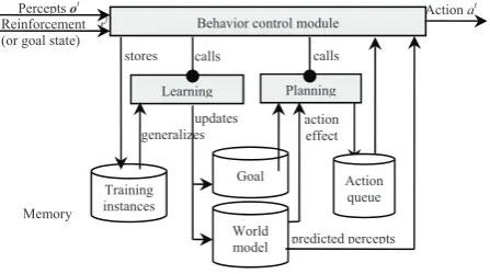
LEAD1 architecture is outlined in Figure 2. Though
the idea of integrating learning and planning in this way is not original but it is quite novel in the context of reinforcement learning (see subsection 3.2.). Each component of this architecture is explained in more detail in the following subsections.
Figure 2. The architecture of the LEAD1 agent
3.1. Learning world model
LEAD1 is based on Markov assumption. It assumes
that any observation ot+1i is a function of the previous
vector of observations ot and of the action at. This
functional relationship is expected to exist for every cell i and to hold for every time instant t.
i fi such that t ot+1i = fi(ot,at) (1)
If discovered, the functions {fi,} would predict
future observations on the basis of past observations
and agents actions. The entire set of functions {fi,}
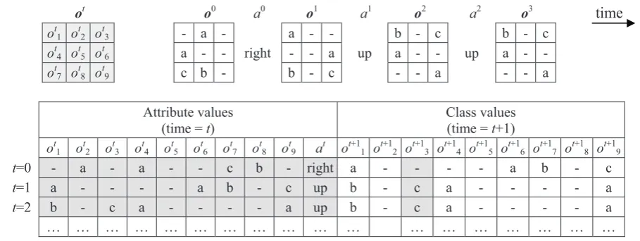
would make up the world model (one function per observation cell). The learner’s task is to discover these functions through supervised learning. A supervised training set is continuously extended at
every discrete time step t out of the triplets of agent’s
elementary experience <ot,at,ot+1>. Parts ot,at of this
experience are taken as attribute values and ot+1i
(individual components of ot+1) are taken as
class-values (Figure 3).
5 Though grid-world cells are organized in a two-dimensional
matrix the observation vector ot obfuscates spatial relationships among individual observations during the supervised learning of the world model.
Behavior control module
Learning Planning
Training instances
generalizes updates
World model Perceptsot
Reinforcement rt (or goal state)
Actionat stores
predicted percepts action effect calls calls
Figure 3. The transformation of the agent’s experience in a 3u3 grid world (top) into the set of training instances for supervised learning of a world model (bottom). Symbols {a, b, c, -} denote grid-world cell labels. The bottom training set is used for learning predictive functions f1, …, f9 (9 learning tasks in total). The area in gray shows one particular training set used to learn
the function f3, such that o
t+1 3 = f3(o
t ,at)
Many supervised learning techniques can be used
to learn the set of functions {fi} satisfying (1). LEAD1
assumes it is operating in a deterministic and observable environment. This means that data noisiness problem can be neglected and suggests decision tree learner as a good candidate for solving
this learning task. Pruning will not be required and decision trees built by the learner will always be
consistent with all training instances stored in LEAD1’s
memory. The outline of LEAD1’s decision tree learner
algorithm is presented below:
BuildTree (Node, Inst, Depth)
// Node – DT Node being processed;
// Inst – set of training instances, associated to Node; // Depth – depth of Node.
IF all members of Inst belong to the same Class THEN Label Node with Class
return(success)
FOR EACH attribute Attrm
IF Attrm values match class values for every member of Inst THEN Label Node with Attrm
return(success)
IF CurrentDepth = MaxDepth6 THEN return(failure)
FOR EACH attribute Attrm
Group the most scattered values of Attrm, into the “other” value Estimate the utility of splitting Inst by Attrm
Sort attributes in the order of decreasing utility FOR EACH attribute Attrm
FOR EACH Attrm value vmi (including the value “other”) Select instances Inst’Inst for which Attrm = vmi result = BuildTree(Successor(Node), Inst’, Depth+1) IF result = failure THEN break
IF result = success return(success) END
6MaxDepthwas set to 3 in our experiments.
The procedure outlined above and resulting decision trees have some differences with respect to
decision trees built by other decision tree builders (e. g. C4.5).
ot o0 a0 o1 a1 o2 a2 o3 time
ot1 ot2 ot3 - a - a - - b - c b - c
ot4 ot5 ot6 a - - right - - a up a - - up a - -
ot7 ot8 ot9 c b - b - c - - a - - a
Attribute values (time = t)
Class values (time = t+1)
ot1 ot2 ot3 ot4 ot5 ot6 ot7 ot8 ot9 at ot+11 ot+12 ot+13 ot+14 ot+15 ot+16 ot+17 ot+18 ot+19
t=0 - a - a - - c b - right a - - - - a b - c
t=1 a - - - - a b - c up b - c a - - - - a
t=2 b - c a - - - - a up b - c a - - - - a
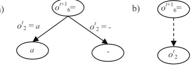
1. Terminal nodes. Besides terminal nodes associated to the pure (in the sense of class labels) subsets of training instances, terminal nodes are created for mixed subsets of training instances if there is an attribute called predictive attribute such that its values match class values of every training instance in the mixed subset. In this case a terminal node is labeled with an attribute name. Labeling nodes with predictive attributes can be thought of as generalizing the structure of a decision tree at the terminal level (Figure 4).
Figure 4. Decision tree predicting ot+1
6 = f6(ot,at) (see Figure 3) by (a) the conventional decision tree builder and (b) by LEAD1. The second tree contains a single node that is
labeled with the name of predictive attribute ot2
2. Aggregating attribute values. Sometimes the split over different values of an attribute results in a few identically labeled terminal nodes. In this case, the attribute values leading to the identically labeled terminal nodes are aggregated together under the “other” branch. If more than one group is present, the larger one is selected for aggregating. This procedure helps to deal with unseen attribute values during percept prediction step (Figure 5).
Figure 5. Decision tree predicting ot+11 = f1(ot,at) (see Figure 3) by (a) the decision tree builder and (b) by
LEAD1
3. Search space and search strategy. Decision tree builders usually follow a “divide and conquer” approach thus performing a hill-climbing, non-backtracking search in the space of possible decision trees. The learner component of LEAD1 performs a depth-first exhaustive search in the space of possible decision trees. The space of decision trees is constrained by the limit that is imposed on the depth of a tree. Failure to create a terminal node within a given depth limit under some branch of a tree causes backtracking. Then a different attribute is selected and sub-trees tied to neighboring branches are invalidated. This search strategy is more costly in computation time but helps in finding more compact decision trees. 4. Node splitting criterion. Node splitting criterion is
used to measure the utility of an attribute for
splitting a particular node. Decreasing order of utility is the order in which attributes are tested during the search. The utility U(A) of the attribute A
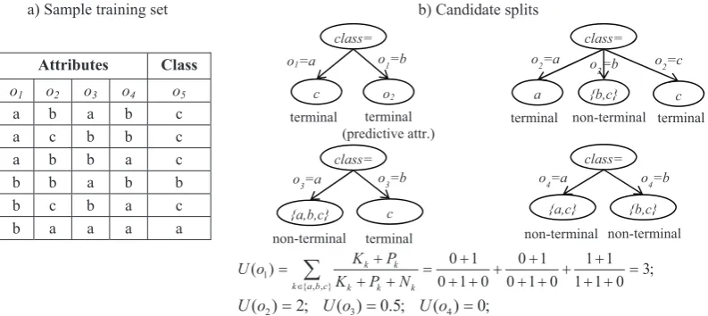
for splitting a particular node is given by (Figure 6):
¦
Classes
k k k k
k k
N
P
K
P
K
A
U
(
)
, where (2)Kk,Pk, and Nk are the quantities of nodes resulting
from the node split over A values such that:
Kk is the number of terminal nodes that would be
labeled by the class k.
Pk is the number of terminal nodes that would be
labeled with a predictive attribute and would cover at least one instance of class k.
Nk is the number of non-terminal nodes that would
cover at least one instance of class k.
The node splitting criterion given by (2) avoids counting training instances in the sub-nodes of the node under investigation. The criterion is in favor of attributes that obtain as many “purely” separated and/or predicted classes as possible (Figure 6).
3.2. Learning goal test
LEAD1 can be provided with the goal either
directly or indirectly. In the first case, the percepts corresponding to the goal state are directly “injected” into the agent. In the second case, the goal is specified indirectly by the signal coming through the reinforce-ment channel. The indirect case is more complicated as the planner requires goal percepts or the goal test to be known prior to planning. To address this problem
LEAD1 is dotted with the capability of constructive
induction7 [8]. Having acted in its environment for
some time, the agent accumulates a set of percept-reinforcement associations {<ot,rt>}.Then it learns to discriminate positively and negatively reinforced percept subsets thus inducing a goal test. This goal test is not discarded but kept and refined across different environments thus implicitly assuming that there are universal laws explaining agent’s reinforcement as a function of agent observations. Goal test induction may result in false generalizations especially if there are too few positive training instances. As a result,
LEAD1 may pursue wrong goals during the initial
epochs of its life.
3.3. Planning
Planning component of the LEAD1 agent is
responsible for finding the shortest action sequence that is expected to achieve agent’s goal. It is based on
the breadth-first depth-limited8 search in the space of
agent’s percepts. The initial state is assumed to
7 This capability is embedded into LEAD1’s learner component but
its details are not covered by this paper. Spatial relationships among individual observations of ot are exploited in this type of learning.
8 The depth limit was set to 15 in our experiments. ot2 =a
ot+16=
a)
-a
ot2 =
-b) ot+16=
ot2
b
a)
b a
ot+11=
ot1 =- o
t
1 =a ot1 = b o
t
1 =other
ot+11=
b
b)
a
ot1 =
Figure 6. Illustration of the node splitting utility function U(A). a) Sample training set b) Four candidate splits based on attributes {o1,o2,o3,o4}. The best split is based on the attribute o1 as it has the maximum estimated utility U(o1) = 3.
correspond to the current percepts. Successor-states are generated on the basis of the world model to date.
3.4. Behavior control module
Behavior control module is responsible for
organizing LEAD1’s behavior at the highest level, i. e.
it is responsible for the interaction of the learner and planner components, action selection, and exploitation
vs. exploration trade-off. The outline of LEAD1’s
behavior control module for one time step is presented below:
Behavior control module (current percepts, reinforcement) static world model
static InstWM // training instances for learning world model static InstGT // training instances for learning goal test static action queue // action set expected to achieve the goal static action // last action taken
static anticipated percepts
action m None
InstWM m Update(<previous percepts, action, current percepts>)
InstGT m Update(<current percepts, reinforcement>)
IF anticipated percepts z current percepts THEN
world model m Learner(world model, InstWM)
action queue m {}
IF Satisfy(current percepts, goal test) THEN IF reinforcement = off THEN
goal test m Learner(InstGT)
action queue m {} ELSE return(action) IF action queue = {} THEN
action queue m Planner(world model, current percepts, goal test)
IF action queue = {} THEN
action m random action
ELSE // exploitation vs. exploration
p m random number, p[0,1] If p < prnd THEN
action m random action
action queue m {} ELSE
action m RemoveTopAction(action queue)
anticipated percepts m Predict(world model, current percepts, action)
return(action) END
b) Candidate splits a) Sample training set
class= class=
class= class=
c o2 a {b,c} c
terminal terminal (predictive attr.)
terminal non-terminal terminal
{a,b,c} c {a,c} {b,c}
non-terminal terminal non-terminal non-terminal
o1=a o1=b o2=a o2=b o2=c
o3=a o3=b o4=a o4=b
Attributes Class
o1 o2 o3 o4 o5
a b a b c a c b b c
a b b a c
b b a b b b c b a c b a a a a
; 3 0 1 1
1 1 0 1 0
1 0 0 1 0
1 0 )
(
} , , { 1
¦
abc
k k k k k k
N P K
P K o
U
; 0 ) ( ; 5 . 0 ) ( ; 2 )
(o2 U o3 U o4
LEAD1
anticipated p i. e. the real-w world model experience. P percepts do n action plan. action seque returns an em
If the pl
LEAD1 selec
action plan, purposes of
that LEAD1 w
action sugges
1
rnd
p
where all_rn
the sliding w
inc_rnd is t
all_rnd acti predicted by decreases as model increa current action 4. Experim The obje was to demo its world mo is capable of capable of o For this reas other adaptiv reinforcemen experimental experimental experimental All agent the size of 9 describing it content label
a tree, and a
of 8 elementa actions, one successful, a within their 1 and 2 c successful if
9 The width of th 10 In other expe
forward and turn
invokes the percepts mism
world experie l and makes Planning com not satisfy the Upon succe ence leading t mpty sequence lanner is una cts a random a random act environment will select a r sted by the pla
1 exp 2 ¨¨ ¨ ¨ ¨ © § rnd rnd all inc
nd is the numb
window of th the number ions that ha y the world m
s the estimat ases. If a rand n plan must b
mental invest
ective of our onstrate that a odel as well as f solving an e operating in a
son, the LEA
ve agents bas nt learning l investigat l setups, com l setup that is ts were place
9u9 cells. Eve
ts content. T ls:an agent,a wall. Agents ary actions: fo e action per
actions go a
environment cells respectiv f the destinatio
he window was s erimental setups,
rn right.
e learner c match the cu ence. The lear it consistent mponent is inv e goal test and ess, the plann to the goal. U e.
able to find a action. Even tion may be s exploration. P random action an is given by
,
01 . 0 ¸¸¸
¸ ¸
¹ ·
ber of random he most recen of random a d their effec model. The p ted reliability dom action is p
e reset.
tigation
r experimenta an agent capa s its goal conc extended set o a wider set of
AD1 agent wa
sed on Q-lear techniques. tion includ mparisons were
described bel ed within an e ery cell was a There were 6
a box,an empt
s had an action
ourgo actions
r possible d
and jump dis
in the specifi
vely. Any g
on cell was em
set to 20 in our ex the agent was g
component urrent percept rner updates th
with the late voked if curren
there is no an ner returns th Upon failure,
an action pla n if there is a selected for th Probability pr
n instead of a y:
(3)
m actions withi nt actions9, an actions amon cts incorrectl probability pr
y of the worl performed, an
al investigatio able of learnin cept descriptio of tasks, i. e. f environment as compared t rning and AD Though ou ded differen e based on th ow.
environment o assigned a lab 6 different ce
ty cell,a stump
n set consistin
s and four jum
irection10. splaced agen ed direction b
go action wa
mpty. Any jum
xperiments. given 2 actions: g
if ts, he est nt ny he it an an he rnd an ) in nd ng tly rnd rld ny on ng on is ts. to DP ur nt he of bel ell p, ng mp If nts by as mp go actio and Agen The mean agen
go ac T agen agen subje actio sight cente expe perc Figu a) In T epoc time its en reach time reinf goal mem know Q-va A techn sche agen defin vs. e yield A tasks summ 11 In o enviro saw h top). frame
12 The
exper
on was succes the intermed nts remained
environment ning that hav nts to reach th ction 9 times. The environme nts through the nts mapped ective coordin on go left cau t” to shift rig er cell of th erimental set eptual frame h
ure 7. Grid-wor nitial percepts. b
The life of a chs each epoc
steps. An ep nvironment. A hed the goal
steps per forcement was
. Agents sta mory, i. e. wit wledge (world alues) was acc Adaptive agen
niques were mes given b nts treated th
ning state ide exploration tr d the best perf All three adap
s of gradu marized by Ta
other experimenta onment state in it himself moving a
Such an experim e hypothesis. e maximum dura riments.
sful if the des diate cell was
in the same ce t was consid
ing no obstac he same cell a
ent was comp eir percepts. H
the environm nates. As a r used the who ght. Agents s heir view at up could n hypothesis11 (F
rld environment b) Agent percep has been perfo
all three age h consisting o poch started b An epoch was or if maximu epoch was e s given only u arted the fir thout any p d model, table cumulated from
nts based on implemente by Russell an
eir percepts ntity. Paramet rade-off funct formance.
ptive agents w ually increa able 1.
al setups, the age ts objective coord round the environ mental setup could
ation of an epoch
stination cell w asn’t a tree o
ell, if any act dered to be cles it was po after repeating
pletely observ However, sens
ment state i result, for ins ole perceptual
saw themselv any time. T not benefit
Figure 7).
nt of the reduced pts after the act ormed.
ents was org of a number o by situating an s terminated i um allowed n
exhausted12.
upon agent rea rst epoch w prior knowle es of stat utili m epoch to ep n ADP and Q
ed according nd Norvig [
ot as an ato
eters of the ex tion were opt
were confron asing compl
ent was given an rdinates. As a res nment (as if view d benefit from th
h was set to 50
was empty or a wall.
ion failed. spherical, ossible for g the same
vable to all sors of the into their stance, the
“view of ves in the Thus, this from the
d size 5u5. tiongo left
ganized in of discrete n agent in f an agent number of . Positive aching the with blank dge. The ity values, poch. Q-learning g to the
14]. Both omic label xploitation timized to
nted to 10 lexity as
access to the ult the agent wed from the he perceptual
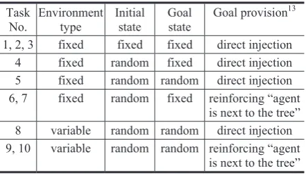
Table 1. Experiment summary Task
No.
Environment type
Initial state
Goal state
Goal provision13 1, 2, 3 fixed fixed fixed direct injection
4 fixed random fixed direct injection 5 fixed random random direct injection 6, 7 fixed random fixed reinforcing “agent
is next to the tree” 8 variable random random direct injection 9, 10 variable random random reinforcing “agent
is next to the tree”
The environment type was denoted as fixed if
contents of its cells were initialized in the same way at the beginning of every epoch. The environment was
denoted as variable if its cells were initialized
randomly using the same six possible cell content labels. The tasks 6-7 and 9-10 were characterized by the environments with more than one goal state. In these environments, all three adaptive agents where reinforced at any state where they found themselves next to some tree.
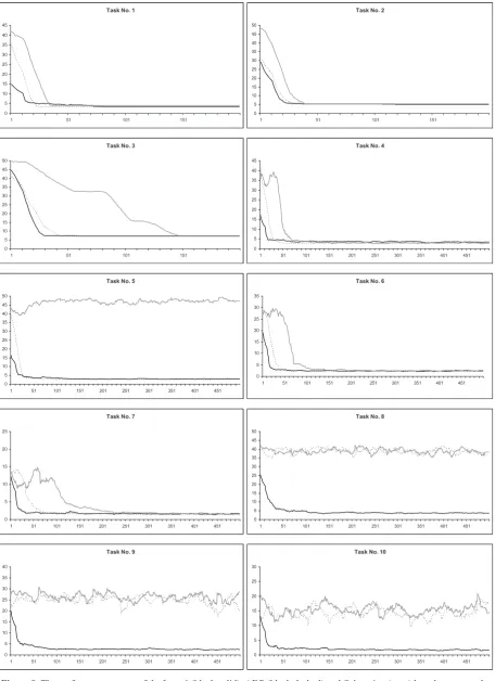
Agent performance was measured through their performance curves (Figure 8).
On the simplest tasks 1-4 all three agents converged to their optimum performance. Q-learning based agent exhibited a slower convergence with the increasing environment size (task 3). Q-learning based agent failed to solve tasks 5, 8-10, which correspond to the changing goal state. This confirms that model-free agents can learn to pursue a single goal. ADP based agent successfully solved the task 5 but failed to solve tasks 8-10. This means that ADP algorithm has mechanisms (world model) to adjust to new goals (the state utility values were cleared and recomputed on the basis of a world model at the beginning of each epoch). Variable type environment presented a challenge that went beyond the generalizing capa-bilities of both Q-learning and ADP. This challenge
was solved by the LEAD1 agent that has learnt explicit
action definitions in terms of its percepts.
LEAD1 solves even those tasks that Q-learning and
ADP cannot cope, but it requires exponential time complexity compared with polynomial complexity of Q-learning and ADP.
5. Discussion and conclusions
The research presented in this paper has shown that it is possible to carry and re-use knowledge acquired in one environment to different environments thus extending the range of tasks solvable by the agent. It has also shown that the planning of action sequences may be a viable action selection policy of the reinforcement driven agents. This paper suggested that one of the ways to address the problem of
13 Only the LEAD1 agent described in this paper was provided its
goal via direct injection. ADP and Q-learning based agents were always provided their goals via reinforcement.
knowledge transferability may be related to the appropriate selection of generalization capabilities of an agent.
The above conclusions are subject to certain limitations and assumptions. First of all, they apply to the class of static, observable and deterministic grid world environments. Second, they assume that meanings of cell labels and agent actions have a universal scope, i. e. that identical cell labels have identical meanings in both seen and unseen grid-world environments. Third, they were demonstrated only for the subset of environments that satisfy the first-order Markov property.
The concerns that LEAD1 that is developed for
static, observable and deterministic environments could not be extended to stochastic, partially observable and dynamic ones are reasonable. However, we believe that there is a way of extending
LEAD1’S behavior to partially observable
environ-ments. The hidden variable approach similar to that used by CALM [13] may be one of the ways to follow. Stochastic perception of the environment (also known as perceptual aliasing) can be thought as a phenomenon arising in consequence to the partial observability of the world and approached by the same method as well.
The assumption of the universality of cell labels and agent actions doesn’t seem to be very annoying. In real-world robotic systems, grid-world cell labels should normally by extracted by the frontend process-ing of sensory data. Though labels may become noisy, the labeling itself should remain consistent.
The agent architecture described in this paper was tested in the environments satisfying the first-order Markov property. It would be straightforward to extend the learning task defined by (1) to include more past percepts: ot+1i = fi(ot-n, …, ot-1,ot,at). This would
theoretically enable the agent to construct world model in the higher order Markov environments. However, the time complexity of learning is an exponential function of the number of parameters. Planning that is based on the breadth-first search is exponentially prohibitive as well. Giving-up the perceptual frame assumption does not allow the agent to use efficient search orienting heuristics like those derived from the means-ends analysis [10]. The limits imposed by the computational costs on the agents’ architecture are still to be investigated.
Another interesting development of LEAD1 would
be to carry it to the Block’s World task [6] [7]. This environment is characterized by composite (parameterized) actions like PutOn(CubeA, CubeB) or PutOnTable(CubeA). It would be interesting to see how such an extension would impact the structure of
Figure 8. The performance curves of the LEAD1 (black solid), ADP (black dashed) and Q-learning (grey) based agents on the tasks 1-10. X axis shows the number of epochs and the Y axis shows the average number of actions to achieve the goal (performance). Y axis values have been averaged over epochs, using sliding window of size 20. In experiments presented results
are averaged in 5 trials
Task No. 1
0 5 10 15 20 25 30 35 40 45
1 51 101 151
Task No. 2
0 5 10 15 20 25 30 35 40 45 50
1 51 101 151
Task No. 3
0 5 10 15 20 25 30 35 40 45 50
1 51 101 151
Task No. 4
0 5 10 15 20 25 30 35 40 45
1 51 101 151 201 251 301 351 401 451
Task No. 5
0 5 10 15 20 25 30 35 40 45 50
1 51 101 151 201 251 301 351 401 451
Task No. 6
0 5 10 15 20 25 30 35
1 51 101 151 201 251 301 351 401 451
Task No. 7
0 5 10 15 20 25
1 51 101 151 201 251 301 351 401 451
Task No. 8
0 5 10 15 20 25 30 35 40 45 50
1 51 101 151 201 251 301 351 401 451
Task No. 9
0 5 10 15 20 25 30 35 40
1 51 101 151 201 251 301 351 401 451
Task No. 10
0 5 10 15 20 25 30
References
[1] Artificial Intelligence Library. A Survey of Cognitive and Agent Architectures. University of Michigan, 2010. Web. 3 May, 2010. Available at: http://ai.eecs.umich.edu/cogarch0.
[2] L. Baird. (1995). Residual algorithms: reinforcement learning with function approximation. In: Proceedings of the 12th International Conference on Machine Learning. Morgan Kaufmann, pp. 30-37.
[3] M. M. Bongard, I. S. Losiev, M. C. Smirnov. Project modeli organizaciji povedenija – Zivotnoje. Modelirovanije. Obuchenija i povedenija. Nauka, 1975, pp. 153-209. (in Russian).
[4] L. De Raedt, H. Blockeel. Using logical decision trees for clustering. In: Proceedings 7th International Workshop on Inductive Logic Programming, 2nd ed. Springer, Berlin, 1997, pp. 133-141.
[5] G. L. Drescher. Made-up Minds: A Constructivist approach to Artificial Intelligence, 2nd ed. The MIT Press, Cambridge, Massachusetts, 2002.
[6] S. Džeroski, L. De Raedt, K. Driessens. Relational reinforcement learning. Machine Learning, 43, pp.7-52 (2001). http://dx.doi.org/10.1023/A:1007694015589. [7] M. Irodova, R. H. Sloan. Reinforcement learning and
function approximation. In: FLAIRS (2005), pp. 455-460.
[8] J. Kapoit-Dzikien, G. Raškinis. Constructive In-duction of Goal Concepts from Agent’s Percepts and Reinforcement Feedback. Information Technology and Control, Vol. 39, No. 3 (2010), pp. 211-219.
[9] J. J. Murray, C. J. Cox, G. G. Lendaris, R. Saeks.
Adaptive dynamic programming. In: IEEE Transaction on Systems, Man, Cybernetics, Part C: Applications & Reviews, 2002, Vol. 32, No. 2, pp. 140-153, http://dx.doi.org/10.1109/TSMCC.2002.801727.
[10] W. Shen, H. A. Simon. Rule Creation and Rule Learning Through Environmental Exploration. In: Proceedings of 11th International Joint Conference on Artificial Intelligence, Palo Alto, California. Morgan Kaufmann, 1989, pp. 675-680.
[11] R. S. Sutton. First results with Dyna, an integrated architecture for learning, planning, and reacting. In: Series In Neural Network Modeling And Connectionism. MIT Press, 1990, pp. 179-189.
[12] R. S. Sutton, B. Tanner. Temporal-Difference Networks. In: Advances in Neural Information Processing Systems 17, 2005, pp. 1377-1384.
[13] F. Perotto, J. Buisson, L. Alvares. Constructivist anticipatory learning mechanism (CALM): Dealing with partially deterministic and partially observable environments. In: Proceedings of the 7th International Conference on Epigenetic Robotics: Modeling Cognitive Development in Robotic Systems, Piscataway, NJ, USA. Lund University, Cognitive Studies, 2007, pp. 117-127.
[14] S. J. Russell, P. Norvig. Artificial Intelligence. A Modern Approach, 2nd ed. Pearson Education, Inc., Upper Saddle River, New Jersey 07458, 2003, pp. 830-859.
[15] C. Watkins, P. Dayan. Q-learning. Machine learning, vol. 8, no. 3, 1992, pp. 279 - 292, http://dx.doi.org/10.1007/BF00992698.
[16] C. M. Witkowski. Schemes for Learning and
Behaviour: a New Expectancy Model. Ph. D. Thesis, University of London, 1997.