A systematic approach for modelling quantitative lake ecosystem data to facilitate proactive urban lake management

R E S E A R C H

Open Access

A systematic approach for modelling quantitative

lake ecosystem data to facilitate proactive urban

lake management

Aaron N Wiegand

, Christopher Walker

, Peter F Duncan

, Anne Roiko

and Neil Tindale

Abstract

Background:The management of the health of urban lake systems is often reactive and is instigated in response to poor aesthetic quality or physicochemical measurements, rather than from an overall assessment of ecosystem health. Interpreting physicochemical monitoring data in isolation is problematic for two main reasons: the suite of parameters that are monitored may be limited; and the contribution that any single parameter has towards water quality or health varies considerably depending on the nature of the system of interest. Extending monitoring programs to include flora and fauna results in a better dataset of ecosystem status, but also increases the complexity in interpreting whether the status is good or poor.

Results:This paper details a process by which a large set of quantitative biological, physical, chemical and social indicators may be transformed into a simple, but informative, numerical index that represents the overall ecosystem health, while also identifying the likely source and scale of pressure for remedial management action. The flexibility of the proposed approach means that it can be readily adapted to other lake systems and environments, or even to include or exclude different indicators. A case study is presented in which the model is used to assess a comprehensive longitudinal dataset that resulted from monitoring a constructed urban lake in Southeast Queensland, Australia.

Conclusions:The sensitivity analysis and case study indicate that the model identifies how changes in individual monitoring parameters result in changes in overall ecosystem health, and thus illustrates its potential as a lake management tool.

Keywords:Modelling, Urban lakes, Ecosystem health, Management, Index

Background

In Australia, design guidelines for urban lakes have been refined over the past few decades to better cater to the impacts associated with urban settings. Current design guidelines consider an urban lake to be a receiving envir-onment for runoff, requiring that the runoff is pre-treated prior to input through various measures (e.g. retention and re-use, constructed wetlands and bioretention basins). While the contemporary design guidelines have been embraced by many levels of authority, difficulties with the subsequent management of urban lakes are still present (Lloydet al.,2002; Bayley & Newton, 2007; Walkeret al.,

2010). Management of urban lakes, and indeed many aquatic ecosystems, is often reactive and is instigated in response to poor aesthetic quality or dictated by physi-cochemical measurements, rather than from an overall assessment of ecosystem health (Rapport, 1998; Karr &

Chu, 1999; Likens et al.,2009). Management strategies

for urban lakes have generally been short term and are often reactionary to physicochemical monitoring alone, which serves to temporarily address an issue, but often fails to provide a long-term solution (e.g. macrophyte har-vesting) (Walkeret al. 2010). Remediation strategies that are based solely upon the limited observations provided by physicochemical monitoring, are likely to have limited effectiveness and may fail to identify and address issues with the broader ecosystem health of an urban lake.

* Correspondence:[email protected] 1

University of the Sunshine Coast, Locked Bag 4, Maroochydore DC, QLD 4558, Australia

Full list of author information is available at the end of the article

Interpreting physicochemical monitoring data as repre-senting good or poor water quality, or even lake health as a whole, is problematic for two main reasons: the suite of parameters that are monitored may be limited; and the contribution that any single parameter has with respect to quality or health is not well identified and may vary considerably depending on the nature of the system of interest. For example, in Australia, existing guidelines, such as ANZECC (2000) and Queensland Water Quality Guide-lines (DERM, 2009) present reference condition values for slightly to moderately disturbed freshwater lakes in Southeast Queensland (SEQ), but these are probably not appropriate or realistic for existing urban lakes, because they assume that urban lakes were once in an undisturbed state or that the influence of an urban catchment is min-imal, as the reference condition values are based on natural lake ecosystems. Additionally, the use of reference condi-tion values can lead to the assumpcondi-tion of an equilibrium, or constant state, while aquatic ecosystems are generally in a state of flux (Reeves & Duncan, 2009), driven by climatic, seasonal or external influences (e.g. stormwater runoff) and changing primary productivity. While urban lakes may demonstrate high quality and health when first constructed, this is generally considered a temporary state in the absence of effective management of the lakes (Leinster, 2006).

A further problem with interpreting a suite of physico-chemical data, is how these may be used to represent the overall quality of the lake system. It is fairly common prac-tice to express the overall quality as a single index or score, by applying a weighting to each monitored quantita-tive parameter that rates each parameter according to the perceived influence of that parameter on overall health (Sanchezet al., 2007; Bordaloet al., 2006; Fernándezet al., 2004). Another approach is to map each measured param-eter value (e.g. concentration of PO4, or temperature) to a normalised index value by use of a graphical function (or lookup table) of parameter value (Cude, 2001).

Cude (2001) utilised eight water quality indicators (dissolved oxygen, biological oxygen demand, ammonia & nitrate nitrogen, total phosphorus, temperature, total suspended solids, pH and faecal coliforms) to establish a model which provided a scaled reference condition for streams in Oregon, USA. The model scored the geomet-ric mean of the selected indicator scores which ranged

from 0 – 100, with a score of 0 –59 considered to be

very poor, 60–79 poor, 80–84 to be fair, 85–89 to be

good and 90 – 100 to be excellent. This modelling

approach linked different indicators to present a concise summary as to the state of health in a stream and whether or not it was appropriate for recreational use. The results were easily communicable and could allow managers to prioritise at-risk areas (Cude, 2001).

Although there is debate regarding the accuracy of using an overall index, the interpretive simplicity of this

approach has resulted in it being used in various forms by many agencies responsible for reporting on the quality and/or health of water systems (United Nations Environment Program, 2007; Hallock, 2002).

In order to evaluate the health status of water-based ecosystems and to pre-empt degradation, an improvement on assessing just physiochemical quality is to also assess biological indicators, which may be more representative of large-scale ecosystem health. A comprehensive study of assessing biological indicators was undertaken by Reiss

and Brown (2005), who developed “a Florida Wetland

Condition Index (FWCI) for isolated depressional forested wetlands in Florida”. Although the detailed approach does not lend itself to be implemented as a routine monitoring program, the study concluded that the inclusion of bio-logical indicators with physical and chemical indicators resulted in a useful index for biological integrity.

Presently, many urban lakes are degraded (Mitsch & Gooselink, 2000; Bayley & Newton, 2007) and, given that many constructed urban lakes are central features of residential developments, it is important to include social and public health indicator data in any evaluation or discussion of lake health (e.g. aesthetic satisfaction, community behaviours, microbial quality, algal and cyano-bacteria risks). Social and health indicators can help assess the value the local residents place on the lake, what impacts community behaviour may have on lake health and what risks such lakes may be having upon the resi-dents and thereby includes the local community as part of the“ecosystem”.

The inclusion of a broader suite of lake-health indica-tors increases complexity. Evaluation of multi-parameter physicochemical data alone can be a difficult task in it-self, and the inclusion of additional data types increases the complexity of the analysis, but carefully designed models can assist with the interpretation of large, com-plex datasets, identify problems that may yet occur and allow for pre-emptive and adaptable management.

While the approaches for reducing a large dataset to a single number are useful, they do not reflect the fact that the overall health of a system is better represented by the worst scoring parameters; individual parameter values that indicate a decline in health are typically “smoothed” and hidden when averaged against many other values. As agencies monitor more parameters, it is likely that the overall average index will become more stable and less sensitive to changes in individual parameters. Models for ecosystem health must be sensitive enough to detect when any part of the ecosystem becomes non-ideal.

how catchment-specific data may be used to more accur-ately describe the health of the constructed lake ecosystem.

Methods

The described approach aims to assist ecosystem man-agers in the development of a modelling tool that may be used to summarise and interpret large sets of disparate data that may result from monitoring practices. The resulting modelling tool itself is not dynamic as it does not make temporal predictions and is not based on differ-ential equations. It is better described as a static model that may be used to summarise and simplify large volumes of disparate data for rapid interpretation and manage-ment intervention. The general approach described in this paper, or even an adaptation of the described model, is designed so it may be incorporated within explicit, tem-poral ecosystem models to provide a temtem-poral“overview” of the health of the simulated ecosystem.

With respect to the constructed lake system to which this approach has been applied, three major groups of measurable environmental indicators (parameters) were identified: water quality; flora; and fauna.

A fourth group, social indicators, such as community

“satisfaction”(which may perhaps be quantified through numbers of complaints to the managing authority), has not been explicitly included in the model. However, an

“aesthetic index” has been derived from specific

mea-sured indicators in the water quality and floral groups. In this case, the derived aesthetic index has been used as a proxy for community satisfaction, and is presented in greater detail within the ‘Model Description’ section of this paper.

Water quality indicators

The water quality group of environmental health indicators include all the standard physical and chemical parameters that are typically measured in monitoring programs, such as temperature, turbidity, salinity, dissolved oxygen, pH and, in this case, additional lab-analysis values for various nutrient species.

For most water quality parameters, some measure of legislation exists which stipulates the quantitative range of values over which each water quality parameter is considered“normal”or healthy. In some cases,“normal” is defined to be based on any existing historical data for the system of interest. In the context of the lakes described in this paper, the relevant guidelines are Australian water quality guidelines, such as the Australian New Zealand

En-vironment Conservation Council’s (ANZECC) guidelines

(2000) and Queensland Water Quality (QWQ) guidelines (DERM, 2009).

As some parameters aren’t monitored routinely by agen-cies and, in some cases, the guidelines vary for different types of water bodies, the model is designed to be flexible

and easily adapted for different guidelines and different situations.

The first step in the approach is to quantify each indi-vidual parameter as being in a state that represents“ideal” or“poor”health. With this aim, the relevant water quality guidelines were used to develop functions with which each measured parameter value (e.g. concentration of PO4, or temperature) is mapped to a Health Index (HI) for that parameter, the scale of which ranges from 0 (zero) to 1 (unity), where 0 represents the worst condition possible and 1 represents a healthy, perfect state.

HIp¼fp vp ð1Þ

Where, for parameterp, the Health Index (HI) is related to the measured value (v) of the parameter by a function (f) that is specific to that parameter.

This approach is not new, but is often implemented through an arbitrary definition of the specific nature of the function. In many cases, the function is simply defined as a line that has been drawn on a graph of HI versus parameter value, based on nothing more than“instinct”, although which is perhaps guided by water quality guide-lines and experience. That is not to say that such graphically-defined functions are not effective, but they lack the rigorous and consistent approach that allows less experienced managers to generate functions suit-able for their local requirements. A more mathematical approach is suggested by which, for each parameter,

“regimes” of parameter values are identified that repre-sent“terrible”(HI = 0),“perfect”(HI = 1) and“dynamic” (HI ranges between 0 and 1). Such piece-wise defined functions are readily described, tested, compared and applied in spreadsheets and models.

Two examples of functions for mapping quantitative water quality parameters to Health Indices, as used in the model described in this paper, are provided in Figure 1 (pH and Total Nitrogen).

The generation of these functions is not an arbitrary process, but follows a general procedure by which exces-sively low and high values are identified first, from either water quality guidelines, scientific literature or historical monitoring data. Using total nitrogen (NTOT) as an ex-ample, a complete absence of nitrogen prevents essen-tial ecological processes from occurring, which results in a lack of vigour or productivity. Conversely, a high concentration of NTOT (1500μg/L) infers an overly vig-orous urban lake ecosystem, to the point where eutrophic conditions may be evident (i.e. very unhealthy). It follows that both a complete absence and a value exceeding

1500 μg/L are both unhealthy and are therefore mapped

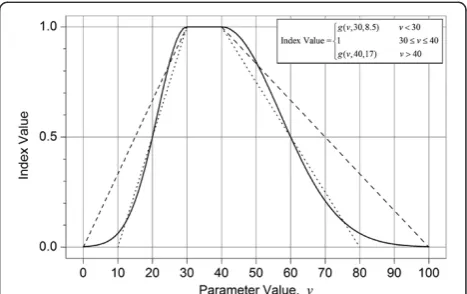
The specific nature of the function as it changes be-tween 0 and 1 is open to debate, but in the absence of spe-cific empirical data, it is necessary to select a function that behaves in a predictable and reasonable manner. The sim-plest option for this purpose is a linear function, but this has the disadvantage of resulting in“shoulders”where the function“pieces”meet and, if the piece-wise defined func-tion is not programmed carefully, may result in negative HI values or HI values greater than 1. This paper proposes that a simplified Gaussian function be used to describe all dynamic sections of the HI function (Equation 2).

HI¼g vð ;v1;wÞ ¼e0:5ð Þvwv1 2

ð2Þ

Where vis the measured value of the parameter (the

variable), v1 is the parameter value at which HI must

equal 1, and w is the width coefficient, analogous to standard deviation.

The selection of this function for the dynamic regimes provides four significant advantages: i) it can be used in the same form for both cases where HI increases from zero to 1 or decreases from 1 to zero; ii) it cannot provide HI values less than zero or greater than one; iii) it provides a smooth continuum across the regimes of piece-wise defined functions and iv) the parameter-specific compo-nents (v1 and w) are readily estimated in a systematic manner.

The width coefficient may be estimated by either of two methods. The preferred method identifies the specific

parameter value at which the health is classed as a“Fail”, ie HI falls below 0.5. Having identified the boundary value of the parameter at which HI is one (v1), identify the value at which the HI must fall to a value of 0.5 (v0.5). The width parameter is then calculated by:

w¼0:85jv1v0:5j ð3Þ

The alternative method for specifying the width param-eter is to estimate the width of the domain over which the HI falls from one to near zero (Δv). The width parameter is simply estimated asw=Δv/3. This is useful when rapid changes in HI are required. The use of this simplified Gaussian function is illustrated in Figure 2.

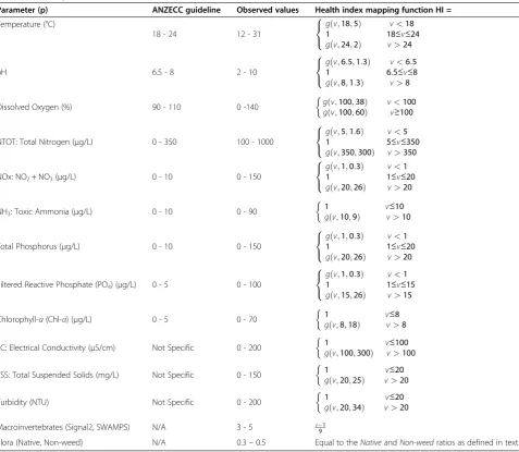
The complete list of HI functions used in the model described in this paper is provided in Table 1. Note that, for any given ecosystem, the list of parameters included in the model can be reduced or extended, depending on what parameters are actually measured and what data are available.

Ammonia presents a unique problem that must be dis-cussed specifically, as it equilibrates between NH3 and

NH4+, the equilibrium being dependent on both pH and

temperature. Although only the NH3 form of ammonia

is toxic, ammonia is typically measured as ‘total

ammo-nia nitrogen’ (TAN), which is the sum concentration of

NH3and NH4+. The fraction of TAN that is NH3can be determined as described in Körneret al.(2001), which is

Figure 1Examples of Health Index (HI) values as functions of ecosystem monitoring parameters pH, total nitrogen and macro invertebrate SWAMPS score.

then used to determine actual NH3(toxic) concentration and subsequently the HI for ammonia (Table 1).

While this approach to processing the water quality indi-cators is similar to Cude (2001), the functions described for this specific application of the model were adjusted to relevant local and regional criteria based upon the re-sponse of a sub-tropical ecosystem to specific climatic conditions. The curves were also adjusted to suit urban lakes, which are not flowing systems, as were measured by Cude (2001).

Once all parameter values are mapped to their respect-ive HI values, they are quantitatrespect-ively summarised to cre-ate the overall wcre-ater quality health index (WQHI). Cude

(2001) suggests that all HI values be summarised by their geometric mean, as this is more sensitive to changes in individual variables than the arithmetic mean. It is im-portant that the WQHI is not positively biased by large quantities of good HI values, and that very poor HI values (e.g. values of 0 which indicate a need for very urgent at-tention) are not“lost”through averaging with better HI values. For management purposes, it is important that the model quickly identifies when any one parameter goes bad, rather than emphasise good health. For these reasons, the WQHI is calculated from the geometric

mean of the ‘worst’ three HI values. The use of the

worst three HI ensures that the WQHI is not too sensi-tive to any single water quality indicator (such as if only Table 1 Model parameters that contribute to the OEHI

Parameter (p) ANZECC guideline Observed values Health index mapping function HI =

Temperature (°C)

18 - 24 12 - 31

g vð;18;5Þ v<18

1 18≤v≤24

g vð;24;2Þ v>24 8

< :

pH 6.5 - 8 2 - 10

g vð;6:5;1:3Þ v<6:5 1 6:5≤v≤8

g vð;8;1:3Þ v>8 8

< :

Dissolved Oxygen (%) 90 - 110 0 -140 g vð;100;38Þ v<100 g vð;100;60Þ v≥100

NTOT: Total Nitrogen (μg/L) 0 - 350 100 - 1000

g vð;5;1:6Þ v<5

1 5≤v≤350

g vð;350;300Þ v>350 8

< :

NOx: NO2+ NO3(μg/L) 0 - 10 0 - 150

g vð;1;0:3Þ v<1

1 1≤v≤20

g vð;20;26Þ v>20 8

< :

NH3: Toxic Ammonia (μg/L) 0 - 10 0 - 90

1 v_≤10

g vð;10;9Þ v>10

Total Phosphorus (μg/L) 0 - 10 0 - 150

g vð;1;0:3Þ v<1

1 1≤v≤20

g vð;20;26Þ v>20 8

< :

Filtered Reactive Phosphate (PO4) (μg/L) 0 - 5 0 - 100

g vð;1;0:3Þ v<1

1 1≤v≤15

g vð;15;26Þ v>15 8

< :

Chlorophyll-a(Chl-a) (μg/L) 0 - 5 0 - 70 1 v≤8

g v_ð;8_;18_Þ v_>8

EC: Electrical Conductivity (μS/cm) Not Specific 0 - 200 1 v≤100 g vð;100;300Þ v>100

TSS: Total Suspended Solids (mg/L) Not Specific 0 - 150 1 v≤20 g vð;20;25Þ v>20

Turbidity (NTU) Not Specific 0 - 200 1 v≤20

g vð;20;34Þ v>20

Macroinvertebrates (Signal2, SWAMPS) N/A 3 - 5 v1 9

the worst indicator was used), and is also not“buffered” or “smoothed” by using a large quantity (or all) of the indicators. The geometric mean is used instead of an arithmetic mean, as an HI of 0 for any of the three worst individual health indices results in an overall index of 0, which emphasises the fact that remedial action is required as a matter of some priority. The geometric mean also emphasises the worst case more than an arithmetic mean and is therefore more appropriate from a management perspective.

WQHI¼ Y 3

i¼1

mini HIp

" #1=3

ð4Þ

Where mini{HIp} is the i’th smallest value in the set of

all HI values.

Floral indicators

Similarly to the WQHI, the overall floral, or vegetation health index (VHI), is calculated from individual HI values, but just two in this case. The first HI describes the proportion of all plants that are defined to be natives (as opposed to exotics), and the second HI describes the proportion of all plants that are defined to be non-weeds. Although highly structured and comprehensive survey methods have been developed for determining health of ecosystems with respect to floral indicator parameters, these are often too expansive and resource-intensive for regular surveys of small systems, especially if they are to be undertaken by local authorities with limited expertise and resources.

In this study, the method for the floral surveys was con-ducted through a simple visual assessment of the riparian and aquatic zones. For the case of urban lakes, a survey may be limited to riparian and visible floating and sub-merged aquatic vegetation. Floating aquatic macrophytes may be surveyed visually from the bank-side of an urban

lake in a 10 m radius point transect (Buckland et al.,

2001). At each survey point, the abundance of each observed plant species was recorded. Each species was then classified as being native or exotic (native species being preferable), and as being a weed species or non-weed species. The latter classification allows non-native species to be non-weeds; ie it simply characterises as favourable those species that do not invade and replace other species. This classification is often straight-forward as many authorities keep registers of known noxious weeds. The HI value of each classification is simply the proportion of all plants that are natives and non-weeds.

For example, if 70% of all the plants are natives, the native-vs-exotic HI value is 0.7; similarly for the non-weeds-vs-weeds HI value. Each HI for the system of inter-est is simply the mean value over all survey points. The VHI is calculated as the geometric mean of the two HIs

to represent the contribution of floral indicators to eco-system health. The geometric mean is used for the same reasons as provided for the calculation of the WQHI.

VHI¼ðHINATIVESHINONWEEDSÞ1=2 ð5Þ

As floral populations do not tend to change as rapidly as, for example, water quality parameters, it is suggested that floral surveys do not need to be performed as frequently, but should be undertaken perhaps biannually or even sea-sonally. Exceptions to this may be following storms, weed harvesting or turnover events, after which some aquatic species may undergo exponential growth, such asSalvinia molestaandNymphaea mexicana.

Faunal indicators

Similarly to the VHI, the overall faunal, or macroinverte-brate health index (MHI), is calculated from only two indi-vidual HI values, each being derived from separate macroinvertebrate survey approaches, as detailed by Chess-man (2003) and Davis et al. (1999). The first approach is

the Stream Invertebrate Grade Number – Average Level

(SIGNAL2), which is typically used on Australian rivers and streams and the second approach is the Swan Wetlands Aquatic Macroinvertebrate Pollution Score (SWAMPS), which is typically applied within Australian wetland ecosys-tems. Each of these survey approaches are used to score the health of rivers, streams and wetlands based upon the diver-sity, type and abundance of macroinvertebrates (Chessman,

2003; Davis et al., 1999) and provide a numerical score

from 1 to 10, 10 representing a healthy system. Because most constructed urban lakes have characteristics of both running (e.g. rivers and streams) and static (e.g. wetland) environments, it is prudent to apply both of these survey approaches. It is entirely possible to use alternative survey methods that are perhaps more suitable to a different eco-system, or perhaps even characterise fauna in a similar manner to the approach described in this paper for floral health indices (native ratio and non-pest ratio), but discus-sion of this is beyond the scope of this paper. This study used SIGNAL2 and SWAMPS, because they are straight forward approaches that are recognised for Australian systems.

Each of the SIGNAL2 and SWAMPS scores are mapped linearly to HI values (Figure 1 and Table 1) and the MHI is equal to the geometric mean of the two HI values. The geometric mean is used for the same reasons as provided for the calculation of the WQHI.

MHI¼ðHISIGNAL2HISWAMPSÞ1=2 ð6Þ

Overall ecosystem health index

like the individual HI values from which it is ultimately calculated, has a range of 0 to 1.

OEHI¼ðWQHIVHIMHIÞ1=3 ð7Þ

As the OEHI is a “summary” of many input

para-meters, it serves as a first indication that something is amiss. If, for example, the OEHI is calculated to have a value of 0.6, it suggests that the manager of the system should identify which specific aspect of the system is in need of attention. It may eventuate that the low OEHI is caused by a single high ammonia value, or a high turbid-ity value, which may not have been noted at the time of analysis and data entry. Alternatively, a low OEHI may be a cumulative result of several parameters slipping to low levels, which indicates a system in decline.

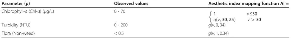
Community (overall aesthetic index)

In addition to characterising the overall health of the ecosystem from measurable environmental factors, the identification of specific drivers for remedial manage-ment is also a goal of this modelling approach. Pressure for remedial action may arise from adverse monitoring results, which will be flagged by the OEHI or, alterna-tively, it may arise from a community’s attitude (for ex-ample aesthetic satisfaction) towards the lakes. It is important that any community surrounding an urban lake is considered in some way to be part of the lake ecosystem, as it is the attitudes of those communities that dictate how they interact with the lakes and this in turn can affect lake health. A community's perception of poor lake health is typically based on visual or odiferous observations, such as high turbidity or algal blooms, and the response will usually manifest itself in the form of direct complaints, either to the managing body or to media. Tracking complaints quantitatively can prove to be difficult and expensive, but if such data are available, these can be readily incorporated into this model by a similar normalisation approach as already described. In this project, no such data were available, so a proxy for community satisfaction has been developed. The overall aesthetic index (OAI) is based on the assumption that community attitudes towards a lake are primarily driven by specific, visually impacting indicators from the water quality and floral index groups. In terms of water qual-ity, turbidity and chlorophyll-aare considered here to be the most appropriate indicators which contribute to the

OAI, as high turbidity is perceived to be“dirty”and high

concentrations of chlorophyll-a are often viewed with

concern, as the water is visibly green. From the floral group, the proportion of plants that are non-weeds was the parameter selected, as a dominance of weed species in Australian urban lakes may often be linked to floating

macrophyte species, such as Salvinia molestaand

Nym-phaea mexicana. The specific functions that map these parameters to individual indices of aesthetic satisfaction (AI) are provided in Table 2.

The model assumes that community dissatisfaction (eg: formal complaints to lake council) is triggered when any one of these three indexes falls below 0.7, so to cap-ture this, the OAI is defined to be the minimum individ-ual AI from turbidity, chlorophyll-aand non-weed flora and is considered poor enough to generate community complaint when it falls below 0.7. While the critical value of 0.7 has been selected somewhat arbitrarily and is an assumption of community values and behaviour, this provides a conservative assessment which better allows for pre-emptive and adaptable management.

OAI¼MIN AIChla;AITurbidity;AINONWEEDS

ð8Þ

Simulated pressure for management action

As already described, the pressure for management ac-tion (PMA) can come from either monitoring data, which describes the physical, biological and chemical health of the system, summarised as the OEHI, or from community complaint due to dissatisfaction with the ap-pearance of the system, summarised as the OAI. Each of these indices may be used to estimate the degree of pres-sure for remedial action, although it is acknowledged that the specific nature of the function is open to debate. It is suggested here that lake managers must respond when OAI falls below 0.7 (to offset anticipated commu-nity complaint at an early stage) or when OEHI falls below 0.5 (which indicates a fail), so in these cases, the index value is assigned to be unity. Otherwise, the de-gree of pressure for remedial action is based solely on the OEHI. This is summarised by Equation 9:

PMAI¼ 1 OAI<0:7 or OEHI<0:5

2ð1OEHIÞ OAI≥0:7 and OEHI≥0:5

ð9Þ

Table 2 Model parameters that contribute to the aesthetic index

Parameter (p) Observed values Aesthetic index mapping function AI =

Chlorophyll-a(Chl-a) (μg/L) 0 - 70

1 v≤30

g vð;30;25Þ v>30

Turbidity (NTU) 0 - 200 g(v, 0, 34)

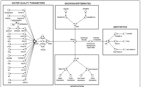
An illustration of the relationships between all parts of the model is provided in Figure 3.

Assumptions and limitations

As with the development of any new modelling approach, there are several assumptions that have been made and these impose inherent limitations on the model (CRC for Catchment Hydrology, 2005).

In the model described in this paper, the specifications that define water quality parameters to be “healthy”, or otherwise, are based on standard Australian guidelines (ANZECC, 2000; DERM, 2009) and on a set of monitor-ing data that was collected over four years. While the Australian guidelines provide reference condition values for slightly to moderately disturbed freshwater lakes, the monitoring data served to inform values more typical of the lake systems of interest. The use of monitoring data to develop specifications for individual water bodies is based on percentiles and is fully described in the above guidelines. The specific correspondence functions that map parameter values and HIs require further refine-ment in order for the model to be applicable to other ecosystems, particularly those with inherently different physicochemical and climatic conditions (e.g. saline lakes and temperate climates). As already described, the spe-cific shape of each function must be defined with care

and, at the very least, undergo qualitative validation that the outcomes are reasonable.

Model sensitivity

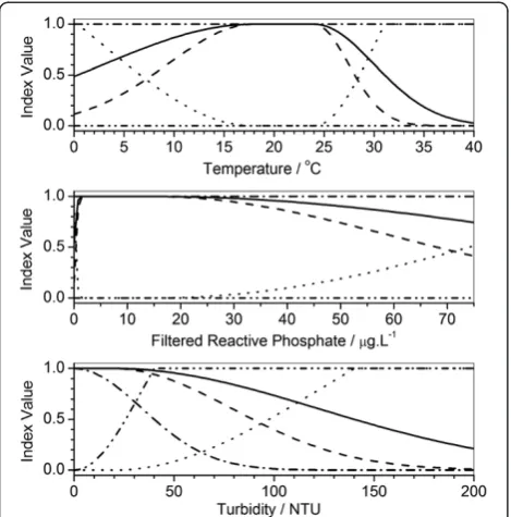
A sensitivity analysis of the model was conducted to deter-mine the sensitivity of the OEHI to the various health indi-cators and which indiindi-cators were most likely to trigger a need for remedial action. All exogenous parameters in the model (indicators) were set to optimum values (HI = 1) and the impact of each individual parameter within all groups (water quality, floral and faunal) was assessed from the lowest to the highest extremes. Examples are pre-sented in Figure 4, which illustrate the sensitivity of the lake ecosystem to temperature, phosphate and turbidity respectively.

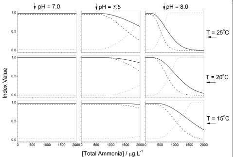
The sensitivity of the overall WQHI to total ammonia was considered in conjunction with temperature and pH. At higher temperatures and pH, ammonia is more persist-ent in its toxic, un-ionised form. As shown in Figure 5, the effect of total ammonia on ecosystem health became more pronounced as temperature and pH increased, with pH having the more substantial effect.

The indicators to which the OEHI was most sensitive to in terms of the full scale of each parameter (i.e. OEHI quickly degraded with increase/decrease over the full range) were found to be temperature, pH, turbidity, filtered

reactive phosphate, total phosphorus, oxidised nitrogen, total nitrogen, total ammonia, chlorophyll-a, dissolved oxygen saturation and the ratio of weed to non-weed floral species. This was to be expected, as the sensitivity analysis is a reflection of the original value-to-HI functions. These indicators trigger more obvious and severe changes in the WQHI and aesthetic satisfaction, and subsequently the OEHI, and are therefore more prone to trigger a need for remedial action, which is essential if the model is to raise alerts when environmental values are not“normal”.

In order to assess the sensitivity of the model to“ nor-mal” conditions, it was also necessary to determine the indicators to which the OEHI was most sensitive over the expected parameter range (20th percentile and 80th percentile from monitoring data). For example, the 20th

and 80th percentile values for temperature were 18°C

and 25°C respectively and the OEHI did not dramatically change in this range, indicating that it was not strongly sensitive to changes in temperature. The OEHI was most sensitive to change in dissolved oxygen saturation and to

a lesser extent, filtered reactive phosphate, over the expected range. While the remaining indicators did im-pact the overall ecosystem health index, such imim-pacts were less obvious and occurred more gradually, particu-larly for conductivity and total suspended solids. This stable behaviour is essential if the model is not to raise alerts for fluctuations in environmental values that are

“normal”.

Results and discussion

In order to assess the applicability and effectiveness of the model with real-world data, a case study analysis was conducted by using the model to summarise an existing multi-disciplinary dataset that resulted from a full year of monitoring several urban lakes. This moni-toring was conducted each month over 2009 (with the exception of March and April due to equipment failure) at the Chancellor Park estate in Sippy Downs, South East Queensland, Australia, which contains a series of ten linked, constructed urban lakes. Results from a spe-cific lake in this estate, Lake 6, are presented here as a case study. Application of this model to other lakes yielded similar results to those presented here.

Site description

The Chancellor Park estate is comprised of medium to heavy residential development, with an extensive commer-cial development of approximately 13 ha which drains to the head of ten linearly-connected urban lakes. The lakes were constructed along the natural drainage line as a cen-tral feature of the residential development. All lakes in the system capture runoff from residential areas and the last lake in the chain discharges into a National Park. The pri-mary functions of the lake system are twofold; the first is to capture and filter runoff from the surrounding urba-nised catchment prior to discharging into a National Park. The second function is to create an aesthetic benefit for the community and provide an area of passive recreation. Of the lakes in the system, Lake 6 was selected to present as a case study as it is situated in the middle of the chained lake system and represents a typical con-structed urban lake (surface area 1.67 ha, maximum depth 3.3 m, volume 26 ML, direct catchment area 67 ha).

Case study results

Water quality monitoring, for each of the water quality parameters listed in the model, was undertaken each month at the input, output and the vertical profile (i.e. the water column) at the centre. Mean values of each in-dicator over all measurements for each month were used to represent the value of that parameter over the entire lake. The values for the macro invertebrate and floral in-dicator groups were comprehensively surveyed only once during the year and therefore were represented as

being constant for the year (no temporal study on these was conducted). In retrospect, although potentially ex-pensive, it is recommended that faunal and floral studies be undertaken at least twice per year to identify any sea-sonal changes, or more frequently if any rapid changes are observed (Figure 6).

Lake 6 demonstrated variability in the WQHI, with some distinction between the WQHI and the OEHI, the latter including the VHI and MHI. Temperatures, NOx, PO4and turbidity were the water quality parameters that had the most influence on the WQHI. In July 2009 and November 2009, the WQHI was less than 0.1 which, unto itself should raise alarm for managers, and also sig-nificantly impacted the OEHI, which is the index that managers would be watching most carefully. The low WQHI in July 2009 was a result of very high turbidity

and PO4 caused by construction works occurring

up-stream from the lake. In general of 2009, it is clear that Lake 6 had a poor OEHI, with a mean of 0.28 from January to December 2009.

The aesthetic satisfaction index was consistently low, driven by the high turbidity and a widespread presence of

exotic floating weed species (Nymphaea mexicana, also

known as the Yellow Waterlily). The lack of aesthetic satis-faction in the model anticipated that community pressure for remedial action would be forthcoming. Regardless, the very low WQHI should trigger a management response even in the case that aesthetic satisfaction had been accept-able. The low OEHI score indicates that the health of the lake should be a high management priority.

The model proved to be sensitive enough to automat-ically identify months in which lake health decreased or improved; closer analysis of the specific monitoring parameters for those months verifies that the model ac-curately reflected the health status of the lake with re-spect to those parameters.

Although the model indicated that there was little tem-poral variation between the overall ecosystem health and water quality indexes, this was likely the result of the static (non-temporal) values entered for the floral and faunal index groups. Although floral communities are less subject to observable change, bi-annual or seasonal surveys will serve not only to identify changes in floral communities, but also the effectiveness of related management strategies

(e.g. weed control). Faunal communities are also subject to change as a result of seasonal shifts and disturbance events, so seasonal macroinvertebrate surveys would allow stake-holders to establish patterns in faunal composition in rela-tion to the other environmental indicators. The inclusion of more robust and variable floral and faunal data would serve to increase the sensitivity of the model to these para-meters.

Model extension

Although the model provided a novel inclusion of the

community in the sense that resident’s attitudes were

simulated by proxy, it was limited in scope and scale. A broader spectrum of community-linked satisfaction indi-cators may yield a more sensitive index to reflect commu-nity behaviours, interaction, satisfaction and/or attitudes towards urban lake ecosystems. For example, parameters may be included that quantify the degree and frequency of physical contact with the lakes, which could be linked to water quality parameters and expressed as a human-health risk index, but such data are not always readily available and further observational or survey type research would need to be undertaken.

Other, more physical parameters that may be included, although only limited data are often available, are micro-bial cyanobacteria and specific faunal hazards (e.g. mos-quito larvae). These relate not only to ecosystem health, but may also be adapted in combination with quantified exposure assessments to provide an estimate of risk to the public and provide a third driver for remedial action.

Looking beyond this model itself, this simple and adapt-able approach for calculating an overall index of ecosystem health directly from measured data, makes aspects of this model highly suitable for inclusion within larger, dynamic models such as those that simulate water quality para-meters as a function of time.

Conclusion

This paper details a flexible approach by which a model may be developed as a means for calculating a single index value (the OEHI) to describe the overall health of a lake ecosystem, which is readily understandable to a range of stakeholders. This overall index is derived from quantifi-able indicator data pertaining to physicochemical water quality parameters, floral surveys, and faunal surveys, which can be collected through a multi-disciplinary inves-tigation of the ecosystem. The described approach is unique for several reasons namely: i) the suggested use of a simplified Gaussian function to define the dynamic regimes of mapping parameter-to-HI (makes extension of the model more accessible to non-experts); ii) the use of only the ‘worst’ three physicochemical water quality HI values for the calculation of the WQHI makes the model more sensitive when individual parameters become poor; iii) floral and faunal indexes are included in a simple man-ner as components of ecosystem health, with equal weighting as physicochemical water quality parameters; iv) simulated community satisfaction is included as a

compo-nent of ecosystem health and “complaint” is generated

whenever any single aesthetic indicator drops below a threshold value. The model also recognises two “drivers”

for remedial action by the managing authority, specifically: monitoring data (usually undertaken by system managers), and community satisfaction. Each driver is handled differ-ently and triggers a need for management action independ-ently. Although the approach described in the paper is not limited to any particular indicator set and can be modified or extended to include additional indicators, it does require knowledge regarding what is considered “healthy” for any given parameter in the system and the specific correspond-ence functions that map parameter values and HIs require further refinement in order for the model to be applicable to other ecosystems, particularly those with inherently dif-ferent physicochemical and climatic conditions.

The included case study presents a specific application of the model in which it is calibrated for urban lakes in South East Queensland, Australia, using Australian guidelines and local monitoring data. Through this, it is demonstrated that the described approach is effective for simplifying large datasets and responds to changes in individual parameters that impact the overall health of the system.

Competing interests

The authors declare that they have no competing interests.

Authors’contributions

AW assisted with collection of field data, designed the modelling approach, prepared and edited much of the manuscript. CW collected the field data, helped develop and test early drafts of the model, performed the literature review, prepared and edited the manuscript. AW, NT, PD and AR secured funding for the project, assisted with the design of the monitoring program and the interpretation of subsequent data, and helped to draft the manuscript. All authors read and approved the final manuscript.

Acknowledgements

The authors gratefully acknowledge and thank the Sunshine Coast Council for the financial support provided towards a monitoring study of lake ecosystem health, from which some data are incorporated in the case study presented in this manuscript.

Author details

1_{University of the Sunshine Coast, Locked Bag 4, Maroochydore DC, QLD} 4558, Australia.2_{School of Ocean Sciences, Bangor University, Anglesey, LL59} 5AB, United Kingdom.

Received: 24 December 2012 Accepted: 1 February 2013 Published: 9 February 2013

References

ANZECC & ARMCANZ (2000) Australian and New Zealand guidelines for fresh and marine water quality. Australian and New Zealand Environment and Conservation Council & Agriculture and Resource Management Council of Australia and New Zealand, Canberra

Bayley ML, Newton D (2007) Water quality and maintenance costs of constructed waterbodies in urban areas of south east Queensland. Proceeding from 5th international water sensitive urban design conference-‘rainwater and urban design. Pub: Engineers Australia, Sydney. ISBN 1877040614

Bordalo AA, Teixeira R, Weibe WJ (2006) A water quality index applied to an international shared river basin: the case of the Colorado river. Environ Manage 38:910–920

Buckland ST, Anderson DR, Burnham KP, Laake JL, Borchers DL, Thomas L (2001) Introduction to distance sampling: estimating the abundance of biological populations. Oxford University Press, Oxford

Chessman B (2003)SIGNAL 2–A scoring system for macro-invertebrate (‘water Bugs’) in Australian rivers, monitoring river heath initiative technical report No. 31. Commonwealth of Australia, Canberra

CRCfor Catchment Hydrology (2005) General approaches to modelling and practical issues on modelling choice. Series on Modelling Choice 1:1–21 Cude CG (2001) Oregon water quality index: a tool for evaluating water quality

management effectiveness. J Am Water Resour Assoc 37:125–137 Davis J, Horwitz P, Norris R, Cheesman B, McGuire M, Sommer B, Trayler K (1999)

Wetland bioassessment manual (macroinvertebrates). National wetlands research and development program. Environment Australia, Canberra Department of Environment and Resource Management - DERM (2010)

Monitoring and sampling manual 2009. Queensland Government, Ver. 2, Available at http://www.ehp.qld.gov.au/water/pdf/monitoring-man-2009-v2. pdf [accessed 08 Feb 2013]

Fernández N, Ramírez A, Solano F (2004) Physicochemical. Water Quality Indices–A Comparative Review Bistua: Revista de la Facultad de Ciencias Básicas 2(1):19–30 Hallock D (2002) A water quality index for Ecology’s stream monitoring program,

vol Publication number 02-03-052. Washington State Department of Ecology, Available at https://fortress.wa.gov/ecy/publications/summarypages/0203052. html [accessed 08 Feb 2013]

Karr JR, Chu EW (1999) Restoring life in running waters: better biological monitoring. Island Press, Washington, D.C.

Körner S, Das SK, Veenstra S, Vermaat JE (2001) The effect of pH variation at the ammonium/ammonia equilibrium in wastewater and its toxicity toLemna gibba. Aquat Bot 71:71–78

Leinster S (2006) Delivering the final product - establishing vegetated water sensitive urban design systems. In: Ana D, Tim F (eds) Book of proceedings: 7th International Conference on Urban Drainage Modelling and the 4th International Conference on Water Sensitive Urban Design: book of proceedings /. Monash University, Melbourne., Australia, pp 1–8 Likens GE, Walker KF, Davies PE, Brookes J, Olley J, Young WJ, Thoms MC, Lake

PE, Gawne B, Davis J, Arthington AH, Thompson R, Oliver RL (2009) Ecosystem science: toward a new paradigm for managing Australia’s inland aquatic ecosystems. Mar Freshw Res 60:271–289

Lloyd S, Wong THF, Chesterfield CJ (2002) Water sensitive urban design–a stormwater management perspective. CRC for Catchment Hydrology 2000:1–44 Mitsch GA, Gooselink JE (2000) Wetlands, 3rd edn. John Wiley and Sons, New York Rapport DJ (1998) Defining ecosystem health. In: Rapport DJ, Costanza R, Epstein

P, Gaudet C, Levins R (eds) Ecosystem health. Blackwell Science, Oxford, UK Reeves GH, Duncan SL (2009) Ecological history vs. social expectations: managing

aquatic ecosystems. Ecol Soc 14(2):8

Reiss KC, Brown MT (2005) Pilot Study—the Florida Wetland Condition Index (FWCI): Preliminary Development of Biological Indicators for Forested Strand and Floodplain Wetlands. Howard T. Odum Center for Wetlands, University of Florida, Gainesville, FL

Sáncheza E, Colmenarejoa MF, Vicenteb J, Rubiob A, Garcíaa MG, Traviesoc L, Borja R (2007) Use of the water quality index and dissolved oxygen deficit as simple indicators of watersheds pollution. Ecol Indic 7:315–328

United Nations Environment Programme (2007) Global drinking water quality index development and sensitivity analysis report., . ISBN 92-95039-14-9 Walker C, Tindale N, Roiko A, Wiegand A, Duncan P (2010) An ecosystem health

approach to assessing stormwater impacts on constructed urban lakes. Refereed proceedings from the National Conference of the Stormwater Industry Association, Sydney, Australia

doi:10.1186/2193-2697-2-3

Cite this article as:Wiegandet al.:A systematic approach for modelling quantitative lake ecosystem data to facilitate proactive urban lake