Calibration of vector network analyzers on the basis of the LRR-method

c

Copernicus GmbH 2003

Advances in

Radio Science

Calibration of vector network analyzers on the basis of the

LRR-method

I. Rolfes and B. Schiek

Institut f¨ur Hochfrequenztechnik, Ruhr-Universit¨at Bochum, Universit¨atsstr. 150, 44801 Bochum, Germany

Abstract. The LRR method for the calibration of vector

net-work analyzers is presented. This method belongs to the self calibration procedures where the calibration circuits might be partly unknown. The LRR calibration circuits are all of equal mechanical length in contrast to the well known TRL cali-bration, which needs a line-standard with a different length than the other calibration standards. For the LRR method it is thus not necessary to displace the connectors of the vector network analyzer during calibration in order to contact the calibration structures. The calibration circuits mainly consist of reflective networks that have to be placed at three consec-utive positions. As the algorithm accounts for different dis-tances between the reflective networks, the circuits are easy to realize. The robust functionality of the LRR method is confirmed by measurements.

1 Introduction

At microwave frequencies the complex scattering parameters of linear devices can be measured with vector network ana-lyzers (VNA). The anaana-lyzers have to be calibrated in order to eliminate systematic errors from the measurement results. For the calibration of a VNA with four receivers it is advan-tageous to use self-calibration techniques where the calibra-tion standards can be partly unknown. The commonly used TRL (Thru Reflect Line) method (Engen and Hoer, 1979; Eul and Schiek, 1991) needs a line-standard that differs in length from the other calibration standards. In order to contact the calibration circuits the distance between the connectors of the VNA has to be changed. Therefore a more complex test-fixture is needed. The TRL method is thus for example not suited for applications where the connector distance is fixed. The LRR method (Line Reflect) solves this problem, be-cause its calibration circuits are all of equal mechanical length. This method can thus be used advantageously for instance in free space systems where a variation of the an-Correspondence to: I. Rolfes ([email protected])

tenna positions might be critical due to changes of the beam propagation. The calibration structures of the LRR method are very similar to the ones of the LNN method (Heuermann and Schiek, 1997). A symmetrical, reciprocal network, the so-called obstacle, is placed at three consecutive positions. While this obstacle network has to show a transmission for the LNN method, the networks of the LRR method consist of reflections, which might or might not show a transmis-sion. The LRR method is thus able to perform a calibration on the basis of reflective networks, which leads to an enlarge-ment of the bandwidth in comparison to the LNN method. The calibration structures of the LRR method can be real-ized very easily as etched structures in microstrip technology or as metal plates for free space applications for instance.

In the following the theory of the LRR method is pre-sented, where in principal two cases are distinguished. In the first one, the obstacles are assumed to show no transmis-sion at all and in the second one, the obstacles might or might not show a weak transmission. Both solutions are described, because depending on the realized calibration structures the appropriate way should be chosen in order to improve the ac-curacy. In addition the algorithm of the LRR method for dif-ferent distances between the obstacle positions is presented.

2 The LRR method

Q Q

l

Q

l ✛

✲ ✲

✛

(a)

Q Q

l1

Q

l2

✛

✲ ✲

✛

(b) Fig. 1. Principal setup of the LRR calibration circuits with (a) equal

and (b) different lengths.

M0=G−1LLH

a2,1=k4ρb2,1, a3,1=ρb3,1

a2,2=k2ρb2,2, a3,2=k2ρb3,2

a2,3=ρb2,3, a3,3=k4ρb3,3

✛ ✲✛ ✲

l l

Fig. 2. LRR calibration structures in microstrip technology.

2.1 LRR method without transmission

For this variant the calibration structures may be realized e.g. in microstrip technology as open-ended transmission lines as depicted in Fig. 2. The calibration circuits can be described with the help of a line parameterk=e−γ lwith the unknown propagation constant γ and a reflection coefficient ρ. The wave parametersa1,i, . . . , a4,i andb1,i. . . b4,i, i = 1. . .3 are defined according to the setup in Fig. 3 where the re-flection coefficientsρl,i andρr,irefer to theidifferent posi-tions of the reflective networks. G and H are two-ports which represent the systematic errors of the VNA. During the self-calibration G and H are eliminated in order to determine the unknown line parameterkand the reflection coefficientρ.

For this purpose the error two-port G−1is described by the following equation withG˜ =G−1:

b1,i a1,i

= ˜G

a2,i b2,i

= ˜G

ρl,ib2,i

b2,i

(1) resulting in a bilinear transformation (Schiek and Gronefeld, 1999).

νl,i= b1,i a1,i

= ˜

G11ρl,ib2,i+ ˜G12b2,i ˜

G21ρl,ib2,i+ ˜G22b2,i =

˜

G11ρl,i+ ˜G12 ˜

G21ρl,i+ ˜G22 (2)

Such a bilinear transformation, also known as M¨obius-transformation, is generally defined as, (Schiek, 1999), xj =

C1yj+C2 C3yj+C4

(3)

G

a

_H

b

a

b

✲

✛

DUT

_✛

✲

a

b

✲

✛

a

b

✲

✛

ρ

✛ ✲

ρ

Fig. 3. Simplified block diagramm of the analyzer setup

where the two variablesxjandyjcorrespond to the measure-ment valueνl,iand the unknown calibration standard param-eterρl,iand the constantsC1, . . . , C4represent the error two port parameters of Eq. (2). Concerning the two-port H a sim-ilar equation can be found on the basis of the wave parameter description in Fig. 3.

a4,i b4,i

=H−1

b3,i a3,i

=H−1

b3,i ρr,ib3,i

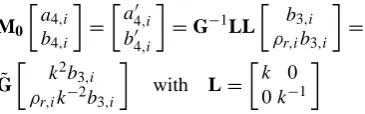
(4) With the help of the first structure of the LRR method in Fig. 2, the through connection with M0=G−1LLH, the de-pendence of the error two port parameter H can be replaced by the error parameterG:˜

M0

a4,i b4,i

=

a_4,i0 b0_4,i

=G−1LL

b3,i ρr,ib3,i

=

˜ G

k2b3,i ρr,ik−2b3,i

with L=

k 0 0k−1

(5) In this way, another bilinear transformation in the error two port parameterG results with˜ ρ˜r,i =k4ρ−r,i1.

νr,i = a_4,i0

b0_4,i = ˜

G11k2b3,i+ ˜G12ρr,ik−2b3,i ˜

G21k2b3,i+ ˜G22ρr,ik−2b3,i =

˜

G11k4ρ_r,i−1+ ˜G12

˜

G21k4ρ_r,i−1+ ˜G22 =

˜

G11ρ˜r,i + ˜G12 ˜

G21ρ˜r,i + ˜G22

(6)

The reflection coefficients ρl,i and ρ˜r,i correspond to the measurement valuesνl,iandνr,i with:

ρl,1=k4ρ⇒νl,1,ρ˜r,1=k4ρ−1⇒νr,1 ρl,2=k2ρ⇒νl,2,ρ˜r,2=k2ρ−1⇒νr,2 ρl,3=ρ ⇒νl,3,ρ˜r,3=ρ−1 ⇒νr,3

(7)

On the basis of the measurement of four reflection coeffi-cients four equations of the type of Eqs. (2) and (6) result, so that the unknown error two port parametersG˜11,G˜12,G˜21 andG˜22can be eliminated. This can be performed with the help of the cross ratio

(y1−y2)(y3−y4)

(y1−y4)(y3−y2)

= (x1−x2)(x3−x4) (x1−x4)(x3−x2)

˜ ν1=

(νl,3−νr,3)(νr,2−νl,2) (νl,3−νl,2)(νr,2−νr,3)

= (ρ−ρ

−1_)(k2_ρ−1_−k2_ρ)

(ρ−k2_ρ)(k2_ρ−1_−ρ−1₎ (9) ˜

ν2=

(νl,3−νl,1)(νr,1−νr,3) (νl,3−νr,3)(νr,1−νl,1)

= (ρ−k

4_ρ)(k4_ρ−1_−ρ−1₎

(ρ−ρ−1_)(k4_ρ−1_−k4_ρ) (10) ˜

ν3=

(νl,3−νl,1)(νr,3−νr,2) (νl,3−νr,2)(νr,3−νl,1)

= (ρ−k

4_ρ)(ρ−1_−k2_ρ)

(ρ−k2_ρ)(ρ−1_−k4_ρ) (11) The line parameter and the reflection coefficient are thus cal-culable as follows:

k4+k2(2− ˜ν1ν˜2)+1=0, ρ2= ˜

ν3−1−k2 k2(k2(ν˜3−1)−1)

(12) 2.2 LRR method without transmission and unequal

obsta-cle distances

In order to account for different lengths between the obstacle positions as shown in Fig. 1b the following algorithm has to be considered. The line elements of the mechanical lengths l1andl2can be described in dependence of the propagation constantγ with the line parameters k1 = e−γ l1 andk2 = e−γ l2 _{and the corresponding transmission matrices L}

1 and

L2. According to Fig. 3 the following wave parameters can be defined:

a2,1=k12k22ρb2,1, a3,1=ρb3,1

a2,2=k12ρb2,2, a3,2=k22ρb3,2

a2,3=ρb2,3, a3,3=k12k 2

2ρb3,3 (13) Considering the previous description of the error two-port

G, Eq. (2) is also valid for this calibration setup. On the

other hand for the error two port H a modified relation re-sults. Starting from Eq. (4) and with H−1=M0−1G−1L1L2 one gets:

M0

a4 b4

=

a₄0 b0₄

=G−1L1L2

b3,i ρr,ib3,i

=

˜ G

k1k2b3,i ρr,ik₁−1k−₂1b3,i

, (14)

so that the following bilinear relation results νr,i =

a_4,i0

b0_4,i = ˜

G11k12k22ρ

−1 r,i + ˜G12 ˜

G21k₁2k₂2ρ_r,i−1+ ˜G22 =

˜

G11ρ˜r,i+ ˜G12 ˜

G21ρ˜r,i+ ˜G22 . (15) For the structures depicted in Fig. 1b with:

ρl,1=k21k22ρ⇒νl,1, ρ˜r,1=k12k22ρ

−1_⇒ν r,1

ρl,2=k21ρ⇒νl,2, ρ˜r,2=k12ρ

−1_⇒ν r,2

ρl,3=ρ⇒νl,3, ρ˜r,3=ρ−1⇒νr,3 (16)

different bilinear relations can be written.

˜ ν1=

(νl,3−νr,3)(νr,2−νl,2) (νl,3−νl,2)(νr,2−νr,3)

=

(ρ−ρ−1)(k2₁ρ−1−k₁2ρ)

(ρ−k₁2ρ)(k₁2ρ−1_−ρ−1₎ (17) ˜

ν2=

(νl,3−νl,1)(νr,1−νr,3) (νl,3−νr,3)(νr,1−νl,1)

=

(ρ−k₁2k₂2ρ)(k₁2k₂2ρ−1−ρ−1)

(ρ−ρ−1_)(k2

1k22ρ−1−k12k22ρ)

(18)

˜ ν3=

(νl,1−νl,2)(νr,2−νr,1) (νl,1−νr,1)(νr,2−νl,2)

=

(k2₁k2₂ρ−k₁2ρ)(k₁2ρ−1−k2₁k2₂ρ−1)

(k₁2k2₂ρ−k₁2k₂2ρ−1_)(k2 1ρ

−1_−k2 1ρ)

(19)

˜ ν4=

(νl,3−νl,1)(νr,3−νl,2) (νl,3−νl,2)(νr,3−νl,1)

=

(ρ−k₁2k₂2ρ)(ρ−1−k2₁ρ)

(ρ−k₁2ρ)(ρ−1_−k2 1k22ρ)

(20)

After some transformations the following equations for the determination of the line parameters and the reflection coef-ficient result:

k2₂±k2 ˜

ν1ν˜3− ˜ν1ν˜2−1 √

˜ ν1ν˜2

+1=0, k1= ±

√ ˜ ν1ν˜3

±√ν˜1ν˜2−k2 ,

ρ2= 1 k₁2

· 1−k 2

1k22+ ˜ν4(k12−1) 1−k₁2k₂2+ ˜ν4k22(k12−1)

(21) The two previously discussed solutions are based on the premise that the obstacle networks show no transmission. For the case that they may have a weak transmission, the following variant of the LRR method is appropriate. 2.3 LRR method with a weak transmission

This algorithm is based on the representation of the obstacle networks with pseudo-transmission matrices. As the obsta-cles might also be realized as pure reflections, the networks cannot be described with transmission matrices, because in this representation a factor1mimight become zero. Accord-ing to Fig. 3 the measurement matrix is defined as follows,

Mi=

_b0

1,i b

00

1,i a0_1,i a00_1,i

₁

a0_4,ib_4,i00 −a00_4,ib_4,i0 _b00

4,i −a

00

4,i −b0_4,i a0_4,i

(22) where the primes indicate from which side of the setup the generator signal is fed in. By multiplying the measurement matrices with the factor1mi =a4,i0 b

00

4,i−a

00

4,ib

0

4,ithe pseudo-transmission matricesQ˜iresult.

˜

Qi=

1mi S21,i

S12,iS21,i−S_11,i2 S11,i

−S11,i 1

=

1 µf,i

µf,iµr,i−ρ2ρ

−ρ 1

The transmission characteristics in forward and reverse di-rection are described byµf,iandµr,i. These values are re-lated to the scattering parameters of the obstacle as follows: µf,i = S21,i/1mi, µr,i = S12,i ·1mi andµf,i ·1mi = 1mi/µr,i taking into account the reciprocity of the obsta-cle. In order to determine the unknown obstacle and line parameters the obstacle networks are positioned as depicted in Fig. 2. Considering the setup in Fig. 1a, the follow-ing pseudo-transmission matrices can be constructed with

˜

Mi=1miMiandQ˜i=1miQ fori=1, . . . ,3: ˜

M1=G−1Q˜1LLH, ˜

M2=G−1LQ˜2LH, ˜

M3=G−1LLQ˜3H (24)

For the obstacle matrices at the different positions it can be found thatQ˜1 = ˆQ/µf1,Q˜2 = ˆQ/µf2andQ˜3 = ˆQ/µf3 whereQ is defined as:ˆ

ˆ

Q=

µf1µr1−ρ2ρ

−ρ 1

=

ˆ q11 qˆ12

ˆ q21 qˆ22

(25) with µf1µr1 = µf2µr2 = µf3µr3 because of the reci-procity.

On the basis of this representation, the following trace rela-tions can be evaluated:

δ1=t r{ ˜M1M0

−1

} =µ−_f11t r{ ˆQ}

δ2=t r{ ˜M2M0

−1

} =µ−_f21t r{ ˆQ}

δ3=t r{ ˜M3M0

−1

} =µ−_f31t r{ ˆQ}

δ4=t r{ ˜M2M0

−1_˜

M1M0−1}

=µ−_f11µ_f−₂1t r{ ˆQLQLˆ −1}

δ6=t r{ ˜M3M0

−1_˜

M1M0

−1 }

=µ−_f11µ−_f31t r{ ˆQLLQLˆ −1L−1} (26) These equations can be transformed into a set of nonlinear equations.

µf1δ1= ˆq11+ ˆq22 (27) µf1µf2δ4= ˆq112 + ˆq

2

22+ ˆq12qˆ21(k2+k−2) (28) µf1µf3δ6= ˆq112 + ˆq222 + ˆq12qˆ21(k4+k−4) (29) The unknown parameters can thus be determined as follows (k+k−1)2= δ1δ6δ

−1

3 −δ12+21m21 δ1δ4δ−21−δ12+21m21 ,

µf1= 1 2h1

·

−h2±

q

h2₂−4h3

,

ρ2=1m2₁µ2_f1−µf1δ1+1 (30) with

h1=δ1δ4δ−21−δ 2 1+1m

2

1(2+h3), h2= −δ1h3,

h3=(k−k−1)2. (31)

a)

a)

b)

b)

(a) (b)

Fig. 4. Obstacle networks (a) without or (b) with transmission.

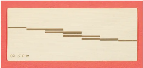
Fig. 5. Foto of the device under test which is a bandpass filter.

As already explained in conjunction with the other methods, an approximate knowledge of the circuits dimensions is nec-essary in order to choose the correct solutions.

3 Experimental results

For the verification of the developed LRR method the ca-libration circuits are realized in microstrip technology.

The obstacles consist of open ended transmission lines as depicted in Figs. 2 and 4. They might also be realized as open ended stubs as shown in Fig. 4. The LRR solution reveals singularities when the electrical length of the line element becomes a multiple of the half wavelength, as is also known from the TRL and the LNN methods.

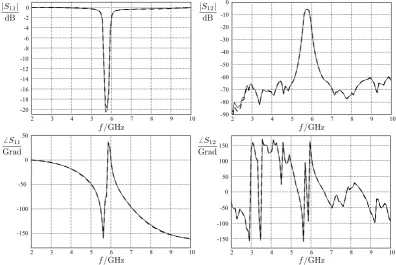
Measurements of a planar stripline bandpass filter as shown in Fig. 5 were performed with a VNA (HP8510C) on the basis of the LRR method in comparison to the TRL method. The measurements lead to similar results which are shown in Fig. 6. The measured scattering parameters show a good agreement between the two methods.

4 Conclusion

|S11|

dB

f/GHz

10 9 8 7 6 5 4 3 2 0 -2 -4 -6 -8 -10 -12 -14 -16 -18 -20

_S11

Grad

f/GHz

50

0

-50

-100

-150

10 9 8 7 6 5 4 3 2

|S12|

dB

f/GHz

0

-10

-20

-30

-40

-50

-60

-70

-80

-90

10 9 8 7 6 5 4 3 2

_S12

Grad

f/GHz

150

100

50

0

-50

-100

-150

10 9 8 7 6 5 4 3 2

Fig. 6. TRL ( ) and LRR method ( ) applied to a bandpass-filter.

References

Engen, G. F. and Hoer, C. A.: Thru-Reflect-Line: An improved technique for calibrating the dual six port automatic network ana-lyzer, IEEE Trans. Microw. Theory Tech., 27, pp. 987–993, Dec. 1979.

Eul, H.-J. and Schiek, B.: A Generalized Theory and New Cali-bration Procedures for Network Analyzer Self-CaliCali-bration, IEEE Trans. Microw. Theory Tech., 39, pp. 724–731, April 1991. Eul, H.-J. and Schiek, B.: Thru-Match-Reflect: One result of a

rig-orous theory for deembedding and network analyzer calibration, Proc. 18th EUMC, pp. 909–914, 1988.

Williams, D. F. and Marks, R. B.: LRM Probe-Tip Calibrations using Nonideal Standards, IEEE Trans. Microw. Theory Tech., 43, pp. 466–469, Feb. 1995.

Heuermann, H. and Schiek, B.: Line Network Network (LNN): An Alternative In-Fixture Calibration Procedure, IEEE Trans. Mi-crow. Theory Tech., 45, pp. 408–413, March 1997.

Schiek, B.: Grundlagen der Hochfrequenz-Messtechnik, Springer-Verlag Berlin, pp. 173–174, 1999.