c
Copernicus GmbH 2003
Advances in
Radio Science
Efficient extrapolation methods for electro- and
magneto-quasistatic field simulations
M. Clemens, M. Wilke, and T. Weiland
Technische Universit¨at Darmstadt, Dept. of Electrical Engineering and Information Technology, Computational Electromagnetics Laboratory (TEMF), Schloßgartenstr. 8, 64289 Darmstadt, Germany
Abstract. In magneto- and electroquasi-static time domain simulations with implicit time stepping schemes the iterative solvers applied to the large sparse (non-)linear systems of equations are observed to converge faster if more accurate start solutions are available. Different extrapolation tech-niques for such new time step solutions are compared in combination with the preconditioned conjugate gradient al-gorithm. Simple extrapolation schemes based on Taylor se-ries expansion are used as well as schemes derived especially for multi-stage implicit Runge-Kutta time stepping methods. With several initial guesses available, a new subspace projec-tion extrapolaprojec-tion technique is proven to produce an optimal initial value vector. Numerical tests show the resulting im-provements in terms of computational efficiency for several test problems.
In quasistatischen elektromagnetischen Zeitbereichsimu-lationen mit impliziten Zeitschrittverfahren zeigt sich, dass die iterativen L¨osungsverfahren f¨ur die großen d¨unnbesetzten (nicht-)linearen Gleichungssysteme schneller konvergieren, wenn genauere Startl¨osungen vorgegeben werden. Verschiedene Extrapolationstechniken werden f¨ur jeweils neue Zeitschrittl¨osungen in Verbindung mit dem pr¨akonditionierten Konjugierte Gradientenverfahren vorgestellt. Einfache Extrapolationsverfahren basierend auf Taylorreihenentwicklungen werden ebenso benutzt wie speziell f¨ur mehrstufige implizite Runge-Kutta-Verfahren entwickelte Verfahren. Sind verschiedene Startl¨osungen verf¨ugbar, so erlaubt ein neues Unterraum-Projektion--Extrapolationsverfahren die Konstruktion eines optimalen neuen Startvektors. Numerische Tests zeigen die aus diesen Verfahren resultierenden Verbesserungen der numerischen Effizienz.
Correspondence to: M. Clemens
(clemens/wilke/[email protected])
1 Introduction
Spatial discretizations of transient quasistatic electromag-netic field formulations with e.g. the Finite Element Method (FEM) or the Finite Integration Technique (FIT), commonly result either in large stiff ordinary differential or index 1 differential-algebraic systems of equations of the form Dd
dtx(t )+K[x(t )]x(t )=b(t ), (1) with theN−component vector x(t )∈ RN whose evolution in time has to be considered over a given time interval. For magneto-quasistatic formulations see e.g. Kameari (1990) or Clemens and Weiland (1999) and for electro-quasistatic systems Preis et al. (2002) or Clemens et al. (2002a).
The solution of (1) requires to use suitable implicit time in-tegration schemes, e.g. one-step schemes such as the simple θ−methods, the multi-stage embedded (singly diagonal) im-plicit Runge-Kutta ((SD)IRK) methods in Cameron (1999) and linear-implicit time integration schemes of Rosenbrock-Wanner-type in Hairer and Wanner (1996) or Lang (2001), which were just recently introduced to quasistatic electro-magnetic field simulations in Clemens et al. (2002c), or the multi-step backward differentiation schemes described in Hairer and Wanner (1996). In these methods in each time step one or several large (non)linear algebraic systems of equations have to be solved. For the iterative solution meth-ods of these systems extrapolation schemes can provide suit-able initial start values. Such first approximations of the so-lutions at the respective new time steps should be computa-tionally cheap to attain and allow to effectively reduce the number of subsequent iteration steps of the preconditioned conjugate gradient solvers. This was shown e.g. in Clemens et al. (2002d), where several extrapolation techniques are compared to produce an initial vector x(n0+1)for the iterative solution x(n+1) ≈ x(tn+1)of the algebraic system at time
t(n+1)
with M= [αD+K],whereαis a scalar parameter depending on the chosen time step length1t.
This paper compares several techniques to improve the nu-merical performance of these algorithms, i.e., to reduce the required number of iterations in the solution methods for the linear algebraic systems of equations as e.g. in the precondi-tioned conjugate gradient (PCG) method. These scheme are here mainly used in the context of FIT-based magnetic field formulations, but extend also to other simulations where im-plicit time integration schemes are used with iterative solu-tion methods. No benefits will arise from the presented meth-ods if direct Gauss elimination schemes are applied which do not require start values.
2 Simple extrapolation techniques in implicit time inte-gration schemes
For each new time step solution x(n+1) ≈ x(t(n+1))of the linear(-ized) system Mx(n+1) =b(n+1) suitable initial solu-tions x(n0+1) for the iterative solution to start on have to be provided. The iterative conjugate gradient solution process is based on a Lanczos orthogonalization where a spectral ap-proximation of the system matrix with tridiagonal matrices is performed as shown in van der Sluis and van der Vorst (1986). Thus the complete reduction of the spectral error components in the approximate solution should not benefit from an available good start solution x0.However, since the
PCG process will be terminated when a user-specified finite accuracy is attained, small error components of the start vec-tors may not require additional iterations. As simple strate-gies for the choice of the start vectors we consider the fol-lowing options that arise with Taylor series expansion ex-trapolations of zero-th order
x(n0+1):=0, (3)
with first order
x(n0+1):=x(n) (4)
or with second order x(n0+1):=x(n)+1t(n+1)d
dtx
(n). (5)
Starting the iterations using a homogeneous start vector x(n0+1) := 0 may be expected to require the most itera-tive work, although it will best allow the conjugate gradient scheme to maintain its weak divergence property for non-gauged, i.e., singular, magneto-quasistatic vector potential formulations (Cp. Clemens and Weiland (1999)). A more commonly used choice of an initial vector for the iterations at timetn+1consists in the solution of the previous time step x(n)under the assumption that provided a short enough time step1t =tn+1−tnthe solutions will not differ too much, i.e., using a first order Taylor approximation. An extension of equation (4) is to choose a second order Taylor expansion which involves the evaluation of the vectordtdx(n).It should
be noted that in magnetodynamic simulations the calcula-tion of the eddy current vectorjec(n+1) = −Mkapdtdx(n
+1)
requires to evaluate these time derivative vectors anyway. If the chosen implicit time integration scheme does not provide an approximation also for dtdx(n+1) it can be calculated sep-arately, for instance by using a second order one-step update scheme
d dtx
(n+1)≈ 2
1t
x(n+1)−x(n)− d dtx
(n) (6)
or using a BDF-formula, as e.g. the multi-step BDF2-appro-ximation
d dtx
(n+1)≈ 1
1t 3
2x
(n+1)−2x(n)+1
2x
(n−1)
. (7) These simple and cost effective to implement start value selection strategies based on the Taylor series expansion can be applied to any suitable implicit time integration scheme.
A similarly simple and seemingly straightforward ap-proach for an extrapolation strategy arises with
x(n0+1):=Me−1b(n+1) (8)
which involves the use of an easily invertible precondition-ing matrix M approximating the system matrix Me . A sim-ple choice is e.g. to take the SSOR-preconditioning matrix e
MSSOR=(D−L)D
−1(D−U), with M=D−L−U.
Since the first step within a PCG method actually consists in the application of (8), no considerable improvements of the process convergence are to be expected from this strat-egy. Numerical tests in Clemens et al. (2002d) confirm this. These simulation results also indicate that using only the start strategy in (4) may be advantageous for constant or nearly constant current excitations whereas the second order Taylor extrapolation in (5) was tested with better results for current excitations with strong variations in the considered time in-terval. Thus it is not initially clear which strategy to follow.
3 Extrapolation techniques for multi-stage SDiRK methods
In the past years, higher order singly diagonal implicit Runge-Kutta (SDiRK) methods were established to be suit-able methods for transient magnetic field simulations in Nicolet and Delinc´e (1996). The increased interest in this family of time integration methods for transient magnetic fields arises from the fact that these one-step methods provide stiffly accurate schemes of almost arbitrarily high order well suited for numerical time integration of differential-algebraic systems of equations of Index 1 of magnetodynamic formu-lations. Ans-stage SDiRK scheme requires to solves (non)-linear algebraic systems of equations to yield the stage vari-ables Yi, i.e., intermediate solution vectors, to be evaluated
at timesti =t(n)+ci1t with
Y(ni +1)=x(n)+1t
i
X
j=1
involving the previous time step solution x(n), the stage
derivatives Y0
i, the SDiRK-coefficient matrix A = {aij}1≤i,j≤s, (aij = 0 for all i < j ). The new time step
solution of the SDiRK-scheme is given by x(n+1)=x(n)+1t
s
X
j=1
bjY0i. (10)
The method coefficient vectors b = {bj}1≤j≤s, c = {cj}1≤j≤s,and the method matrix A completely specify the
chosen SDiRK method. The internal multi-stage construc-tion principle in some cases also allows to construct em-bedded schemes corresponding to a second coefficient vec-torb to provide an additional solution of a lower order. Inˆ Cameron et al. (1998) a stiffly accurate, L-stable 4-stage SDiRK3(2) scheme of third (embedded scheme: second) or-der was proposed and its use for the purposes of an error-controlled variable step length time integration of the dis-crete magnetodynamic systems based on Finite-Element and Finite Integration method formulations was further refined in Wang et al. (2001) and Clemens et al. (2002b).
For the SDiRK schemes we consider the following strate-gies to choose a suitable start value. The most simple extrap-olation formulation is given with a first order Taylor series expansion extrapolation
Y(ni,0+1) :=x(n), (11)
where the last time step solution x(n)is taken as start value for each stage variable vector to be calculated for the next time step.
It is, however, also possible to use the intermediate solu-tions of the internal SDiRK-stages to construct extrapolated start vectors Y(ni,0+1) for the solution at the new time step t(n+1). An extensive mathematical treatment of these tech-niques is found in Cameron (1999), where a stage extension extrapolation method is described with
Y(ni,0+1):=
x(n): i=1,
Y(nl +1):forcl=max1≤k<i{ck|ck≤ci} ci−cj
ck−cjY (n+1)
j +
ck−ci ck−cjY
(n+1) k :
ci forcl ≤cj ≤ci ≤ck≤cm
for alll≤j, k < i;k≤m
, (12)
where a start solution for the corresponding stage value vec-tor is constructed using already available stage values of the current time step 1t(n+1) = t(n+1) −t(n). Not for ev-ery SDiRK method the coefficients ci of the intermediate
timest(n)+ci1t(n)increase monotonically in size such that
ci ≤ cj, i > j, holds. Thus, either an already available
previous stage value is used as start solution or an interpola-tion is performed using the nearest in time stage values Yj
and Ykwithcj ≤ ci ≤ ck following a method described in
Cameron (1999). Note, that certain methods allow to con-sider two stage variable vectors Yi,Yj, i 6= j,at the same
time point in the integration interval, i.e.,ci =cj.
A variant of this approach is the continuous extension ex-trapolation scheme. The solution vectorsx at times¯ t? = t(n)+1t(n)+ci1t(n+1):=t(n)+σi1t(n),
can be extrapolated from the stage derivatives of the last time step by
Y(ni,0+1):= ¯x(t?)=x(n)+σi1t s
X
j=1 ¯
bj(σi)Y0i, (13)
which involves a coefficient vector b¯ = { ¯bj}1≤j≤s, to
achieve the extrapolated stage variable Y(ni,0+1) of the new time step.
For the SDiRK3(2) scheme the following extrapolator co-efficient set is available from Cameron (1999) with
¯
bT(σ ):= 1 30
1σ σ2
22
√
2+15 236−159 √
2 1−7 √
2 135 √
2−222 −14
√
2−15 135 √
2−262 13+14 √
2 264−135 √
2 2
√
2+5 16+20 √
2 −9−7 √
2 −12−15 √
2
.
Note, that one-stage SDiRK schemes are closely related to the standard one-stepθ−methods described e.g. in Hairer and Wanner (1996). For these time integration methods the strategies in Eqs. (11) and (12) will coincide with method (4) and strategy (13) is identical to method (5). Another specific advantage of stiffly accurate SDiRK arises from the fact that in these methods we have the last intermediate time step co-efficientcs = 1,such that Y0s = Y
0(t(n+1)) ≈ d dtx(t
(n+1))
holds. Accordingly, no additional evaluations for the time derivative vectors dtdx(t(n+1)have to be performed.
4 Hybrid extrapolation techniques
All the start vectors x0,i, i = 1, ..., m,derived from the
ex-trapolation techniques described above for the iterative solu-tion of (2) are computasolu-tionally cheap to attain, but numerical test in Clemens et al. (2002d) indicate that just one extrapo-lation method used for the generation of start values may not be suitable for all kind of transient problems.
In order to solve this problem, in Clemens et al. (2002d) already a minimal residual norm selection criterion has been proposed for a set of start values x0,i, i = 1, ..., m,
con-structed with different extrapolation methods. In this min-imal norm hybrid extrapolation scheme first the norms of residual vectors for the different start solutions x0,i are
eval-uated with low additional computational costs. The vector x0,jcorresponding to the smallest residual norm is chosen as
a start vector:
ri := kMx0,i−b(n+1)k2, i=1, . . . , m, x(n0+1) :=x0,j, forj : rj = min
i=1,...,m
{ri}. (14)
The numerical tests show that this approach, while rather simple, is surprisingly effective for a robust reduction of the required computational work independent of the current ex-citation form.
B
r
JrS
(2) (1)
TEAM 11 Hollow Sphere
(3)
r
TEAM 21b
Path 1 Path 2
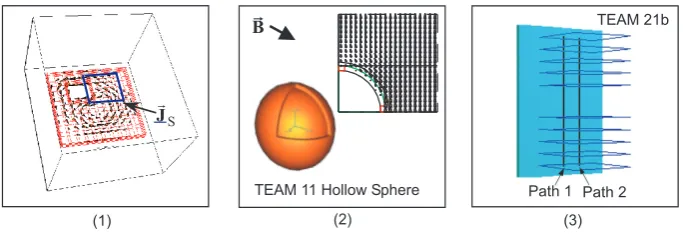
Fig. 1. Three eddy current test problems: 1) A copper plate with a hole: Time harmonic eddy currents in a conductive plate. 2) The TEAM
11 problem: A conductive sphere in an abruptly started homogeneous vertical magnetic field 3) The TEAM 21b problem: Time harmonic eddy currents in a ferromagnetic nonlinear iron plate.
Table 1. Extrapolation strategies for a fixed time stepping BDF1-scheme. The numbers denote the total number of matrix-vector-multiplications during the complete time integration process.
Problem No. 1 No. 2 No. 3
(a) Taylor 1st order x(n0+1):=x(n) 3424 6663 -(b) Taylor 2nd order x(n0+1):=x(n)+1tx˙(n) 2554 16730 -(c) Minimal norm hybrid method for (a), (b) 2714 6703 74392 (d) SPE scheme using (a), (b) (m=2) 923 2889 41182
For this we require that the system matrix M in (2) has to be symmetric and positive (semi-)definite, which is com-monly the case in discrete electro- and magneto-quasistatic field formulations. Here the initial vectors x0,i, i=1, ..., m,
are orthonormalized using a Modified Gram Schmitt proce-dure (see e.g. Meister (1999)) to yield the vectors v0,i, i =
1, . . . ,m,˜ which form a orthonormal basis to a vector sub-spaceVm˜ =span{vj} =span{x0,i} ⊆RN which is spanned
already by all the different start vectors x0,i. Since the
or-thonormalization process will detect linear dependencies in themoriginal vectors x0,i,the relationme≤mwill hold.
With the definition of the orthonormal operator V := {v1|...|vm˜} ∈RN× ˜m,we can restrict the system (2) ontoVm˜
[VTMV]z=VTb(n+1). (15)
to achieve an optimal approximative solution x(n0+1) := Vz of (2) insideV
e
m.Note, that the solution of (15) commonly
involves ame× e
mmatrix withme100N.Thus a direct Gauss elimination process can be adopted and the inverse [VTMV]−1of the system matrix is available. With this the subspace projection extrapolation can be summarized as
x(n0+1):=V[VTMV]−1VTb(n+1). (16) For the resultant initial vector x(n0+1)the Galerkin condition VT[b(n+1)−Mx(n0+1)] =0 holds w.r.t.V
e
m.Such a Galerkin
condition is also essential for the construction of the iterative conjugate gradient solution process.
The subspace projection extrapolation scheme essentially yields an optimal start solution for the system (2) restricted to the linear subspace Vem ⊂ RN spanned by the different
start vectors x0,i.In principle it may occur that there is no
reduction of the iteration steps for the start values generated with this SPE method if the subsequently applied conjugate gradient process is considered as an exact method. Bene-ficial effects, however, will arise in approximative solution processes, where the iterations are terminated once a pre-scribed accuracy for the relative norms of the residual vectors kMx(nk+1)−b(n+1)k/kMx(n0+1)−b(n+1)k ≤εPCGis reached. For many electro- or magneto-quasistatic problems de-scribed with (1) the matrix M = M(x)will, however, de-pend on the solution vector. Such behavior arises with the simulation of nonlinear ferromagnetic materials in magneto-quasistatic problems or field-dependent conductivities in transient electro-quasistatic simulations. While the subspace projection extrapolation initially is derived as optimal start value generation scheme only for linear problems, in this nonlinear case it can be used to perform a few nonlinear fix-point iteration stepsk=0,1, ...,
VTM(x0,k)Vzk+1=VTb(n+1), x0,k+1:=Vzk+1, (17)
where this iteration is started for k = 0 with x0,0 := x(n).The iteration (17) corresponds to that of a Successive-Approximation method restricted to the subspaceVme.
5 Numerical results
Table 2. Extrapolation strategies for the adaptive SDIRK3(2)-scheme from Cameron (1999). The numbers denote the total number of
matrix-vector-multiplications during the complete time integration process.
Problem No. 1 No. 2 No. 3
(a) Taylor 1st order x(n0+1):=x(n) 4636 12310 70647 (b) Taylor 2nd order x(n0+1):=x(n)+1tx˙(n) 4473 10925 69946 (c) Stage-extension extrapolation 3877 7466 58799 (d) Continuous extension extrapolation 4145 10778 66660 (e) Minimal norm hybrid method for (a),(c),(d) 3777 6688 55198 (f) SPE-scheme using (a),(c),(d) (m=3) 2743 6572 35743
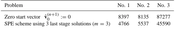
Table 3. Extrapolation strategies for the adaptive linear–implicit scheme RODAS3(2) described in Clemens et al. (2002c). The numbers
denote the total number of matrix-vector-multiplications during the complete time integration process.
Problem No. 1 No. 2 No. 3
Zero start vector vˆ(n0+1):=0 8397 8135 87277 SPE scheme using 3 last stage solutions (m=3) 4766 5537 45590
in Clemens and Weiland (1999). Problem 1 is related to the TEAM 7 problem, a copper plate with a hole featur-ing a ramped 50 Hz sinusoidal current excitation simulated for 80 time steps. Problem 2 is a hollow conductive, non-ferromagnetic sphere in an abrupt B-field (TEAM 11) inte-grated with 40 time steps. Problem 3 consists of the TEAM 21b problem, a nonlinear 50 Hz time harmonic eddy cur-rent problem, simulated over 50 time steps (see also Clemens et al. (2002d)).
In Table 1 the effect of the new SPE method is displayed for the commonly used implicit BDF1 method and in Table 2 for a time-step adaptive 4-stage SDIRK3(2)-method intro-duced in Cameron (1999). The solution of the linear alge-braic systems is performed with a SSOR-preconditioned CG method which terminates its iterations after having reached a relative accuracyεPCG=10−5. The comparison of the dif-ferent start strategies is given in terms of the required total number of matrix vector multiplications (MxV-operations) for the time integration process. This number corresponds well to the required computational time.
The results for both the standard fixed time step BDF1-scheme as well as the adaptive SDIRK3(2)-BDF1-scheme show that the application of the SPE scheme speeds up the solution pro-cess by a factor≥ 2 for linear problems when compared to just using the 1st order Taylor expansion, i.e., starting the PCG-iterations with the old solution x(n0+1):=x(n).The new SPE approach also outperforms all the other extrapolation methods presented above. The convergence of the nonlin-ear problem, in which 4 nonlinnonlin-ear SPE-cycles are performed before entering the nonlinear iteration scheme, is also con-siderably improved.
In Table 3 results for the linear–implicit time integration method RODAS3(2) described in Lang (2001) or Clemens et al. (2002c) are depicted. Its intermediate stage solutions,
for which only linear systems have to be solved, no longer have interpolating character. Thus the extrapolation schemes available for SDIRK-methods are not directly applicable and zero start vectors are commonly used. The application of the new SPE scheme to its respective three last stage solutions (m=3), however, allows to achieve a considerable speed-up of the PCG solver convergence.
6 Conclusion
For transient quasistatic electromagnetic field simulations with implicit time stepping schemes algorithmic improve-ments are presented. Different extrapolation techniques for new time step solutions are compared in combination with the preconditioned conjugate gradient algorithm. Simple extrapolation schemes are suitable for all standard implicit time integration schemes. Their ideas extend to specialized schemes for multi-stage implicit Runge-Kutta time stepping schemes. With the subspace projection extrapolation tech-nique a new hybrid techtech-nique is proposed which allows to choose an optimal initial value independent of the problem dynamics at only moderate additional costs. Numerical tests illustrated the resulting improvements of the computational efficiency for several transient magnetodynamic problems.
References
Cameron, F.: Low-Order Runge-Kutta Methods for Differential Al-gebraic Equations, Ph.D. thesis, Tampere Univ. of Technology, 1999.
Clemens, M. and Weiland, T.: Transient eddy current calculation with the FI-method, IEEE Trans. Magn., 35, 1163–1166, 1999. Clemens, M., Gersem, H. D., Koch, W., Wilke, M., and Weiland,
T.: Transient simulation of nonlinear electro-quasistatic prob-lems using the Finite Integration Technique, in Proceedings of the 10th International IGTE Symposium on Numerical Field Cal-culation in Electrical Engineering, 2002, Graz, Austria, pp. 510– 515, 2002a.
Clemens, M., Wilke, M., and Weiland, T.: 3D transient eddy current simulations using FI2TD with variable time step size selection schemes, IEEE Trans. Magn., 38, 605–608, 2002b.
Clemens, M., Wilke, M., and Weiland, T.: Linear-implicit time inte-gration schemes for error-controlled transient nonlinear magnetic field simulations, in Proc. CEFC,2002, Perugia, p. 332, to appear in IEEE Trans. Magn. (scheduled May 2003), 2002c.
Clemens, M., Wilke, M., and Weiland, T.: Extrapolation strategies in transient magnetic field simulations, in Proc. CEFC 2002, Pe-rugia, p. 331, to appear in IEEE Trans. Magn. (scheduled May 2003), 2002d.
Hairer, E. and Wanner, G.: Solving Ordinary Differential Equations II, Stiff and Differential-Algebraic Problems, Springer, Wien,
New York, 1996.
Kameari, A.: Calculation of transient 3d eddy current using edge elements, IEEE Tr. Magn., 26, 466–469, 1990.
Lang, J.: Adaptive Multilevel Solution of Nonlinear Parabolic PDE Systems: Theory, Algorithm and Application, Springer-Verlag, Berlin, Heidelberg, New York, 2001.
Meister, A.: Numerik linearer Gleichungssysteme, Vieweg-Verlag, Braunschweig, Wiesbaden, 1999.
Nicolet, A. and Delinc´e, F.: Implicit Runge Kutta methods for tran-sient magnetic field computation, IEEE Trans. Magn., 32, 1405– 1408, 1996.
Preis, K., B´ır´o, O., Supancic, P., and Ticar, I.: FEM simulation of thermistors including dielectric effects, in Proceedings of the CEFC 2002, Perugia, Italy, 16.–19. June, edited by E. Cardelli, 2002.
van der Sluis, A. and van der Vorst, H. A.: The rate of convergence of conjugate gradients, Numer. Math., 48, 543–560, 1986. Wang, H., Taylor, S., Simkin, J., Biddlecomb, C., and Trowbridge,