R E S E A R C H A R T I C L E
Open Access
Reduced order modeling for transient
simulation of power systems using
trajectory piece-wise linear approximation
Muhammad Haris Malik
1*, Domenico Borzacchiello
1, Francisco Chinesta
1and Pedro Diez
2*Correspondence:
1Institut de Calcul Intensif (ICI),
École Centrale de Nantes, 1 rue de la Noë, BP 92101, 44321 Nantes Cedex 3, France Full list of author information is available at the end of the article
Abstract
This paper concerns the application of reduced order modeling techniques to power grid simulation. Swing dynamics is a complex non-linear phenomenon due to which model order reduction of these problems is intricate. A multi point linearization based model reduction technique trajectory piece-wise linearization (TPWL) method is adopted to address the problem of approximating the nonlinear term in swing models. The method combines proper orthogonal decomposition with TPWL in order to build a suitable reduced order model that can accurately predict the swing dynamics. The method consists of two stages, an offline stage where model reduction and selection of linearization points is performed and an online stage where the reduced order
multi-point linear simulation is performed. An improvement of the strategy for point selection is also proposed. The TPWL method for a swing dynamics model shows that the method provides accurate reduced order models for non-linear transient problems. Keywords: Model order reduction, Power grid, Swing dynamics, POD, TPWL
Background
Transient stability of the power grids is a keen area of research because of its implications in the power system planning, operation and control. Energy based methods for the transient analysis of power grids were developed originally by Mangnusson [1] and Aylett [2]. The substantial size of power grids makes the transient analysis computationally costly to simulate and therefore a need of model order reduction arises. Reduced order models need to be computationally cost-effective while retaining considerable accuracy of the full model in large network grids simulations.
A number of approximation schemes are available for model reduction and selection of an appropriate scheme depends upon the problem to be solved so that a suitable reduced order model is achieved [3]. Some of the earliest methods in the domain of model order reduction are Truncated Balance Realization proposed by Moore in 1981, Hankel-norm reduction published in 1984 by Glover [4], proper orthogonal decomposition (POD) [5], assymptotic waveform evaluation, PRIMA [4] and a more recent proper generalized decomposition (PGD) [6].
©The Author(s) 2016. This article is distributed under the terms of the Creative Commons Attribution 4.0 International License (http://creativecommons.org/licenses/by/4.0/), which permits unrestricted use, distribution, and reproduction in any medium, provided you give appropriate credit to the original author(s) and the source, provide a link to the Creative Commons license, and indicate if changes were made.
The techniques defined by Bai et al. [3] includes Krylov-subspace techniques, Lanczos based methods such as MPVL algorithm and SyMPVL among others for the reduced order modeling in the electromagnetic applications. The study by Parillo et al. [7] presents the use of POD to reduce the hybrid, nonlinear model of a power network. The authors used the “Swing Equations” which are the differential-algebraic equations of second order to simulate the cascading failures in power systems. They employed model order reduction in parts of the system that remains unaffected by the failures. POD based model order reduction has found applications in diverse fields and is the preferred method in electrical engineering applications such as in the study by Montier et al. [8]. In their study, POD is applied in combination with discrete empirical interpolation method.
Kashyap et al. [9] have used model order reduction for the purpose of state estimation of phasor measurement units (PMUs). The authors have proposed an algorithm based on reduced-dimension matrices which operate separately on PMU measurements and on conventional measurements. The proposed scheme is applicable to distributed imple-mentation and is reported to be numerically stable. The algorithm was applied on a IEEE 14-bus system and compared with existing schemes in the literature and demonstrated good accuracy. Wille-Haussmann et al. [10] used symbolic reduction approach to model lower order grid segments. The study shows reduction by a factor of 2 for a typical grid.
The main hurdle in the effective model order reduction of the power grids is the strong nonlinearity appearing in swing dynamics models. Trajectory Piecewise-Linear method (TPWL) is a well-defined method for the model order reduction of nonlinear time varying applications [11]. This method proposes a suitable strategy for treatment of nonlinearities which presents the real bottleneck of model order reduction. This method has been applied on several nonlinear problems especially to electronics engineering applications [12–19]. A similar method to the one adopted in this paper is found in the work of Bugard et al. [20] and Panzer et al. [21] who have proposed a parametric model order reduction. The main idea presented in these works is to reduce several local models and then produce a parametric reduced order model using a suitable interpolation strategy. Compared to these methods, TPWL has one global reduced basis and uses interpolation of locally linearized models just to represent the nonlinear term in the reduced variables space. More than one training trajectories can be added together to form the single global reduced basis similar to the concept of POD.
TPWL method has been implemented in non-linear control of integrated circuits and MEMS [14]. Xie and Theodoropoulos [22] have used the capability of TPWL of reducing large scale non-linear dynamic models and demonstrated it through the stabilisation of the oscillatory behavior tubular reactors as the case study.
Trajectory piecewise-linear methods are not limited to just power electronics and con-trol systems applications, indeed there are vast areas of research where the application of TPWL based model order reduction will be beneficial [23,24]. The study by He et al. [23] involves the implementation of TPWL macromodeling for subsurface flow simulations. In another study by Cardoso and Durlofsky [24] the work on model order reduction using TPWL methods for subsurface flow simulations is presented.
inefficient with respect to time consumption. Therefore, the adoption of TPWL method in the current study is suitable for the model order reduction of power grids.
The article has been divided into three sections, where “Swing dynamics equations” sec-tion discusses about the mathematical model of the power grid. “Model order reducsec-tion” section deals with the model reduction techniques of POD and introduces the method of TPWL adapted for the swing model. “Numerical experiments” section provides a couple of test cases as an example and the robustness of the application of TPWL method.
Swing dynamics equations Problem statement
A mathematical model to describe the transient dynamics of power systems is the “Swing Dynamics” [25]. It involves a second order differential equation representing the generator node or bus which originates from the rotor dynamics of the generator and an algebraic equation associated with the load bus. The differential equation for theith bus:
miδ¨i+diδ˙i=pmi −pi for i=1,. . ., N (1)
The unknown in the Eq. (1) isδi(t) andivaries fromi = 1,. . ., N whereN represents
the number of nodes in the system. The variablesδi represent the generator rotor angle
derivations with respect to a synchronously rotating frame, while ˙δiand ¨δiare respectively
the first and the second time derivatives of the rotor angle. The quantitiespmi andpiare the
mechanical power input and the electrical power output and are given. The parameters
mianddiare theith generator’s normalized inertia and damping coefficients.
The expression for the electrical power output is given by:
pi=
N
k=1
|Vi||Vk|biksin(δi−δk) for i=1,. . ., N (2)
In Eq. (2)Vi = |Vi|eιδi, andyik = gik +ιbik represents the complex admittance matrix
withbik is the line susceptance andgik is the line conductance, it is assumed that voltage
magnitudes|Vi|do not change and the transmission line losses are negligible, i.e.yik is
purely imaginary (gik =0). Using Eq. (2) in Eq. (1) gives,
miδ¨i+diδ˙i=pmi − N
k=1
|Vi||Vk|biksin(δi−δk) for i=1,. . ., N (3)
Equation (3) describes the transient dynamics of the power system under the assumption that the lines are purely reactive and voltage magnitudes are kept constant [7] since all the nodes are considered as PV nodes.
In the current study, POD is employed for the purpose of model order reduction. It is to be noted in the framework of POD mathematical manipulations of system (3) are more easily handled using matrix and vector representations. Hence, we present the system of equations in matrix form:
[M]{δ¨} +[D]{δ˙} = {pm} − {p({δ})} (4)
Numerical integration of the high fidelity model
Swing equations are numerically integrated in the commercial software MATLAB. A built-in function ‘ode15s’ has been used in the evaluation of the time dependent ODE represented in Eq. (4), because of the potential stiffness of the problem this is the most effective ODE solver available in MATLAB. It is based on the numerical differentiation formulas (NDF) and optionally use backward differentiation formulas (BDF) and is a multistep solver. A detailed description of this method and its incorporation in MATLAB environment is provided in the article by Shampine and Reichelt [26].
Model order reduction Proper orthogonal decomposition
Proper Orthogonal Decomposition is an “a posteriori” method for model order reduction. The objective is to find an orthonormal basis considerably smaller as compared to the high fidelity model using the information extracted from previously computed simulations. Say δis a vector of dimensionNcontaining all the state variables of the system, the objective of POD is to reduce the dimension fromN toqwhereq N. The mapping from the original to the reduced coordinates is expressed by the linear application:
{δ} =[ ˜U]{z} (5)
where {δ}is aN ×1 vector, [ ˜U] is aN ×q matrix, and{z}is aq×1 vector. The goal of POD is to compute matrix [ ˜U] from the analysis of the principal components of the available solutions.
The matrix [ ˜U] can be calculated using several techniques. In essence, POD is similar to the Karhunen–Loeve decomposition (KLD) and it is often referred to as KLD, principal component analysis (PCA) or the singular value decomposition (SVD) [27]. In the current study, SVD interpretation has been used to obtain a reduced order model.
Here, we will briefly describe the SVD reduction procedure which is available as a built-in function built-in MATLAB.
A selection of solution “snapshots” {δ}k, withk = 1,2,. . ., n, are arranged into the
columns of the matrix [Q]∈RN×n,
[Q]=[{δ}1,{δ}2,. . .,{δ}n] (6)
The number of snapshots must guarantee that they represent the complete set of solutions, i.e.,nmust be large enough. The set ofnsnapshots contains redundant information that have to be suppressed by keeping only the pertaining remaining modesq.
The factorization under SVD is given as:
[Q]=[U][][V]∗
=
N
i=1
σi{Ui}{Vi}T ≈ q
i=1
σi{Ui}{Vi}T
(7)
where, [U] is aN×Nmatrix, [] is aN×ndiagonal matrix with non-negative real numbers on the diagonal, and [V]∗is an×n, unitary matrix, [V]∗is the conjugate transpose of then×nunitary matrix [V]. The left hand side of Eq. (7) accurately estimate the full [Q] matrix for i = 1, …, N. The last sum is the truncation of first terms that sufficiently approximates the full [Q] matrix.
of modesq are selected such that for anyj > q, the quotientηis within some defined tolerance andσj σ1, where quotientηis defined as the difference of the relative energy retained, whereη=0 means that the total energy of the system is retained. It is usually the case that only few of the largerσjcontain the most energy and the restσjforj=q,. . ., N
can be dropped from the reduced basis.
η=
q j=1σj
N k=1σk
−1
(8)
The quotientηis employed to find the size of the reduced basis which accurately mimics the original basis, typical values are between 10−1and 10−5. The matrix [ ˜U] is given as:
[ ˜U]=[{U}1,{U}2,. . .,{U}q], q<N <n (9)
The columns of [ ˜U] correspond to vectors{U}irepresenting the most characteristicmodes
in the solution, that is, the most recurrent structures.
For detailed insight into the method and the variations in the above mentioned pro-cedures of KLD, PCA and SVD, the author refers to the studies by Liang et al. [27]. Additionally one can also refer to Kerschen et al. [28] and Berkooz et al. [29].
The reduced order model for the governing equations is obtained by replacing{δ}with the relation given by Eq. (5) in Eq. (4),
[M][ ˜U]{¨z} +[D][ ˜U]{˙z} = {pm} − {p} (10)
and using Galerkin method to project the residual on the reduced basis
[ ˜U]T[M][ ˜U]{z} +¨ [ ˜U]T[D][ ˜U]{z} =˙ [ ˜U]T{pm} −[ ˜U]T{p({δ})} (11)
Defining the following notations
[M] :=[ ˜U]T[M][ ˜U] [D] :=[ ˜U]T[D][ ˜U]
{pm}:=[ ˜U]T{pm}
{p({z})}:=[ ˜U]T{p({δ})}
(12)
we obtain the governing Eq. (4) in the reduced basis as:
[M]{z} +¨ [D]{z} = {˙ pm} − {p({z})} (13)
Note that{p}is a nonlinear fuction of{z}.
Although it is possible to use POD on nonlinear problems for model order reduction, the necessity of evaluating the nonlinear function renders it less practical in terms of computational complexity. In the current study, we are using MATLAB based ODE solver ‘ode15s’, which requires that the nonlinear function to be defined analytically. Recall the Eq. (2) describing the nonlinear function
pi=
N
k=1
|Vi||Vk|biksin(δi−δk) for i=1,. . ., N
The nonlinear function here depends upon the original basisδ, in the reduced basis it has to be defined as:
pi( ˜U z)= N
k=1
|Vi||Vk|biksin
⎛ ⎝q
j=1
( ˜Uij−U˜kj)zj
⎞
⎠ for i=1,. . ., N
˜
pl(z)= N
i=1 ˜
Uilpi( ˜U z) for l=1,. . ., q
The nonlinear function ˜p(z) in the reduced basis therefore becomes,
˜
pl(z)=
N
i=1 ˜
Uil
N
k=1
|Vi||Vk|biksin
⎛ ⎝q
j=1
( ˜Uij−U˜kj
⎞
⎠zj) for l=1,. . ., q (15)
It is evident from the Eq. (15), it requiresO(N2×q2) operations, which is counter-productive to the reduced order modeling. To save computation costs and truly exploit the benefits of reduced order modeling, it would be necessary to eliminate theN2number of operations which is the dimension of original basis. Therefore, a method of trajectory piece-wise linear method (TPWL) has been proposed that is described in the following section.
As an example of the problem with increased computational cost, we performed a simulation with POD based reduced model, the same simulation is presented later in detail. The full simulation without the model reduction required around 202 s, with POD and the nonlinear function as defined in Eq. (15) the simulation took about 290 s.
Trajectory piece-wise linear method
An approach based on TPWL method has been adopted in the current study to reap the benefits of reduced order modeling while also maintaining a good approximation of the nonlinear function.
Evaluation of{p˜(z)}requiresN2×q2operations which results in similar time consump-tion as high fidelity model. The objective of introducing TPWL method is to construct a locally affine mapping{L˜p(z)}fromRqtoRqat some time stepsswheres nwhich
involves less operations and such that{L˜p(z)} ≈ {p˜(z)}.
Trajectory piece-wise linear method is a method combining the model order reduction and the linearization of the non-linear functions. The system in the current study given by Eq. (1) has strong non-linear characteristic and as described in earlier sections, nonlinear reduced order model does not reduce the time consumption. The TPWL method provides a combination of linearized models obtained at selected snapshots.
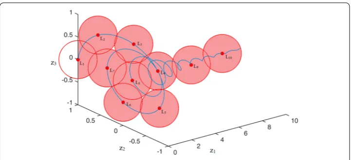
To accurately capture the behavior of nonlinear function, it is important that the points selected for the linearization should be such that they span the whole manifold in which the system trajectories evolve. As an example of this, Fig.1shows the typical trajectory in the space of reduced variable{z}and in this the selection of linearization points is made to ensure that the trajectory is completely covered.
Steps of TPWL Simulation
TPWL method can be separated into an offline and an online stage. The steps during the offline phase are below:
• Step 1: Simulation of the high fidelity model used as the training trajectories (See details in “Selection of training trajectories” section).
• Step 2: Generation of reduced basis using POD.
Fig. 1 Linearization points on a sample curve in reduced basis (z1,z2,z3)
• Step 4: Reduction of the linearized system and the storage of{δ}j,{p˜}j,[˜J]j andS, wherejis the element in the set of linearization pointsS.
Once the above steps are performed and we have a reduced linear system with{δ}j,{p}˜ j,[˜J]j andSavailable, we can perform the simulation of the reduced system in an online phase of TPWL. The following steps comprise the online phase of TPWL.
• Step 1: Load the stored reduced basis. • Step 2: Calculate weighting functions.
• Step 3: Combine the linearized systems in a convex combination. • Step 4: Solve the reduced linearized system.
In the following sections we will present the methodology to select the linearization points and also the weighting procedure for the combination of the linearization points.
Selection of training trajectories
Training trajectories form an integral part of the TPWL method which theoretically, should be able to cover all the domain of the nonlinear function. The selection of train-ing trajectories, therefore, requires careful selection of initial conditions upon which the trajectories of the swing model depend. One may consider it is inefficient to compute so many nonlinear functions to cover the whole domain. However, in practice there are only a few possible conditions a system can achieve in real time applications. Training trajectories provide the points at which the nonlinear system has to be linearized (see “Selection of linearization points” section). It is to be stressed that the TPWL method can interpolate between the training trajectories but not to extrapolate. Therefore, it is necessary to include all the trajectories in the training set that are considered to be visited by the nonlinear function [30].
Selection of linearization points
information already available from the training trajectories. Therefore, we present the equations in terms of the original basis {δ}, the nonlinear function{p(δ)}in Eq. (4) is linearized at certain points in time. This function at a generic snapshot is given by local approximation{Ljp({δ})}as:
{Ljp({δ})} ≈ {p}j+[J]j
{δ} − {δ}j for j=1,. . ., s (16)
This is the first step in the TPWL simulation after the full nonlinear solutions have been obtained at the predefined training trajectories. The initial conditions are represented by
{δ}0and it is by default the first point selected for the linearization. The Jacobian is given by matrix ‘[J]’ as:
[J]= ∂{p} ∂{δ} =
∂{p}
∂δ1 . . . ∂{p}
∂δN
(17)
Note that, the jacobian can be derived analytically for the swing equations.
The linearized function approximates the actual nonlinear function using the Jacobian at the specified linearization points, represented byjin the superscript. The idea behind the TPWL method is that a number of linearization points are selected and the linearized functions at those snapshots are summed up by a weighting function given a global approx-imation as presented in Eq. (18). A detail on the selection of linearization points has been presented in Algorithm 1
{Lp({δ})} ≈ s
j=1
wj·{p}j+[J]j{δ} − {δ}j (18)
where,Lpis the linear approximation,{p}j, [J]jare the nonlinear function and Jacobian
matrix evaluated at thejthlinearization point, and{δ}jis thejthlinearization point. The weight ˆwjis given by (19), which depends on the distancedjbetween{δ}and linearization point{δ}j, and the normalized form is denoted bywjwhich appears in Eq. (18).
ˆ
wj=e−βdj/dmin (19)
whereβis a positive constant and it can be adjusted to reduce the error and smooth the affine function{Lp},djis the distance between{δ}and linearization point{δ}janddminis
the minimum amongdj.
The strategy to select the linearization points is traditionally based on the difference between the phase differences between the successive time steps, i.e., (δi−δi−1)j−(δi−
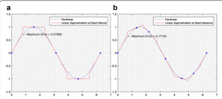
A simple nonlinear trigonometric function and its linear approximation based on the concept of fixed distance in the context of its norm is plotted in Fig.2a while a new method developed in the current study is shown in Fig.2b . As it is observable from Fig.2a and b , the number of linearization points are comparable as 5 in the first case to 7 in the current case has reduced the approximation error by about 40%. Generally, the increase in number of linearization points is of no significant loss in computation time as the selection is done during the offline phase while in the online phase the computation of linear functions is very quick.
This approach is similar to the method proposed in the study of Liu et al. [12] in which the authors have used a global maximum error for linearization point selection.
The modified version of the selection of linearization points is more time consuming then the original method proposed by Albunni [30]. However, selection of linearization points is performed during the offline phase where time is not a constraint, the proposed method in the current study has higher accuracy with the problem discussed here.
A very important note that the nonlinear function{p˜}jand the Jacobian matrix [˜J]jare
stored in the reduced basis.
Weighting function
TPWL method combines the linearized model in a convex combination approximating the original nonlinear system. In a convex combination all the coefficients are greater or equal to zero with the sum of all the coefficients equal to one. If there are ‘s’ linearized models and ‘q’ is the order of the linearized system, then the computation of these weights is in the order ofO(sq) (for detailed study on the weighting function refer to thesis of Rewienski [11]). The calculation of weights is carried out during both the online and offline phases in the current study.
Given the set of linearization pointsSandβ, the weights can be calculated for any point with respect to the points in the linearization set. The value ofβ should be a positive constant, in the current study its value is 25 . A smaller value smooths the function and make its appearance continuous, while a higher value results in kinks in the function. The necessity of adjustingβis that it helps to reduce the error between the nonlinear function and its approximation. The first step is to compute the distancedj between a point{δ} and all the points in the setSusing,
dj= ||{δ} − {δ}j||2 for j=1,. . ., s (20)
The weights are then calculated as,
ˆ
wj=e−βdj/dmin for j=1,. . ., s (21)
where,dmin=min
j=1,...,s dj
Once, the weights are calculated with respect to all the points in the setS, the weights are normalized as:
wj= wˆ
j
s i=1wˆi
, for j=1,. . ., s , i=1,. . ., s (22)
During the online phase, in place of{δ}reduced basis{z}is used to calculate the distance and the points in the setSconsists of linearization points in the reduced basis as well.
Numerical integration of the reduced model
Once a linear model has been obtained from the training trajectories during the offline phase, the values of the nonlinear function and the Jacobian matrix evaluated at the selected linearization points are reduced and stored to be used during the online phase along with the set of linearization points. The nonlinear function and the Jacobian is projected in the reduced space as:
{p˜({z})} =[ ˜U]T{p({δ})}
[˜J]=[ ˜U]T[J][ ˜U] (23)
Since, we replace the nonlinear function with an approximation containing sum of lin-earized functions, we have
{L˜p({z})} =[ ˜U]T{L
p([ ˜U]{z})}
⇒ {L˜p({z})}≈
s
j=1
wj·
{p˜}j+[˜J]j
{z} − {z}j
(24)
In the above equation, the weightswjare evaluated afresh in the reduced dimension. The weights are calculated exactly as described in the “Weighting function” section with {z} replacing the{δ}.
Numerical experiments
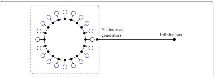
The network grid studied here is termed as the “Ring Grid” consisting of only generators with one reference node connected to all the generators, represented in Fig.3. The math-ematical model describing the ring grid is the swing dynamics given by the Eq. (1). The grid in this study is a ring grid containing all the generator nodes and a slack node in a topology such that the slack node is connected with all the generators. A slack node or bus in electrical power system is a bus where both|V|andδare known and is used to balance the power losses or power demand shortage while performing a power flow study [32]. Here, the slack bus is modeled as an infinite bus which is a simplifying assumption that the voltage at this bus is always constant and it has infinite power capacity as the impedance is zero for this bus. A list of assumptions for the grid in the current study are:
• The power grid is loss-less
• The generators are small and the ratio between the length of transmission line joining generators to the infinite bus and the length of transmission line joining two consecu-tive generators is much bigger. Hence, the interaction between a generator and infinite bus is much smaller than the interaction between two neighboring generators • Transmission lines joining two consecutive generators is shorter than the line joining
the generators with the infinite bus
• Transmission lines between the infinite bus and all the generators are of same length • Transmission lines connecting the generators are of same length
The nonlinear functionpiin Eq. (1) is different from its form given in Eq. (2) due to the
assumptions described earlier and is given as:
pi=bsin(δi)+bint[sin(δi−δi+1)+sin(δi−δi−1)] fori=1,. . ., N (25)
where,bis line susceptance between generators and the reference node andbintis the line
susceptance between two connected generators. The Eq. (1) takes the following form
miδ¨i+diδ˙i=pmi −bsin(δi)−bint[sin(δi−δi+1)+sin(δi−δi−1)]
fori=1,. . ., N (26)
The grid studied consists of 1000 generators and one slack node connected to all the generators. The data used in the study is given in Table 1, all the values are given in per-unit system.
N identical
generators Infinite bus
Table 1 Grid data
Symbol Description Value
mi Mass of the generators 1 (p.u.)
di Damping of the generators 0.25 (p.u.)
pm Power generated by the generators 0.95 (p.u.)
b Susceptance between generator and slack node 1 (p.u.)
bint Susceptance between consecutive generators 100 (p.u.)
N Number of generators 1000
The values used in the current study are adapted from the study of Susuki et al. [33] with the addition of damping to ensure the steady state stability of the power grid. Also, the number of generators in the study of Susuki et al. are only 20 and the focus of their study is to demonstrate the coherent swing instabilities. Although different from the study by Susuki et al., the grid loop as described in their study presented a good opportunity to showcase the ability of TPWL method for the model order reduction and fast simulation of electrical power grids.
Training trajectories and reduced order models
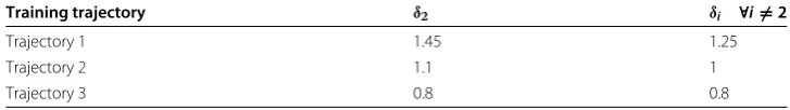
In the current study, there are three different scenarios of initial conditions that must be taken into account for the training trajectories, these are listed in Table3. The dependence of the trajectories on the initial conditions is evident since the trajectory will be different in each case.
As described in “Selection of Training Trajectories” section, multiple training trajec-tories have been employed for the generation of reduced order models. These training trajectories were categorized into three different types. The total time of simulation and the step size are listed in Tables2and3lists the perturbation amount and the node for each case.
1. Initial conditions at the equilibrium point for all the generators bar one.
2. All the generators start from a non-equilibrium point and one generator out of synchronicity.
3. All the generatros start from the same non-equilibrium state and are synchoronous.
Table 2 Training trajectories data
Symbol Description Value (s)
T Total time of simulation 50
T Time step 0.005
Table 3 Initial conditions
Training trajectory δ2 δi ∀i=2
Trajectory 1 1.45 1.25
Trajectory 2 1.1 1
The Jacobian is a tri-banded diagonal matrix in the case under study here.
Jk,l = ∂
pk
∂δl =
∂ ∂δl
bsin(δk)+bintsin(δk+δk+1)+bintsin(δk−δk−1)
=ˆδk,l{bcos(δk)} + {bintcos(δk−δk+1)}(ˆδk,l−δˆk+1,l)
+{bintcos(δk−δk−1)}(ˆδk,l−ˆδk−1,l) (27)
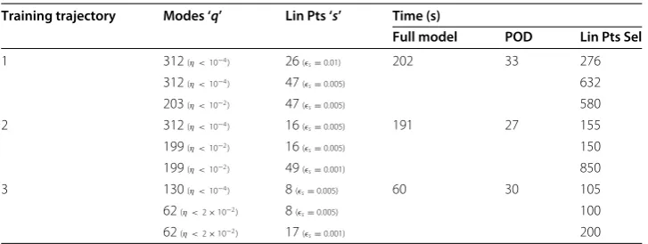
It is intuitive that the more the number of modes and the number of linearization points the more time the reduced model takes to simulate. The time consumption data along with number of modes and linearization points of the training trajectories is listed in Table4. It is to be noted that all the simulations were run on a laptop with a i5-4200 CPU with a 1.6GHz processor and 8 GB RAM.
The comparison between the reduced linearized model from TPWL and the full non-linear model was carried out on the averageδ, which is termed as collective-phase variable and its time derivate isω. These are defined for loop power systems as:
δ = 1 N
N
i=1
δi (28)
ω= dδ
dt =
1
N
N
i=1
ωi (29)
The variables are well-known in power system stability analysis as the Center of Angle (COA) or Center of Inertia (COI) [33]. These variables demonstrate the collective dynam-ics of the system and are useful in the study of stability of the power grids.
The modes and the linearization points from the training trajectories were saved and then used with cases which are slightly different from the training cases. The results we obtained are encouraging for this kind of model order reduction for the nonlinear functions.
First test case: single node perturbation in non-equilibrium conditions
This is the case which is closely related to the second training trajectory. We have all the nodes starting from a non-equilibrium pointδi=1∀i =2 and in addition one node was
perturbed by about 0.12 radians, i.e.,δ2 = 1.12. The initial conditions used for this test case are presented in Table5.
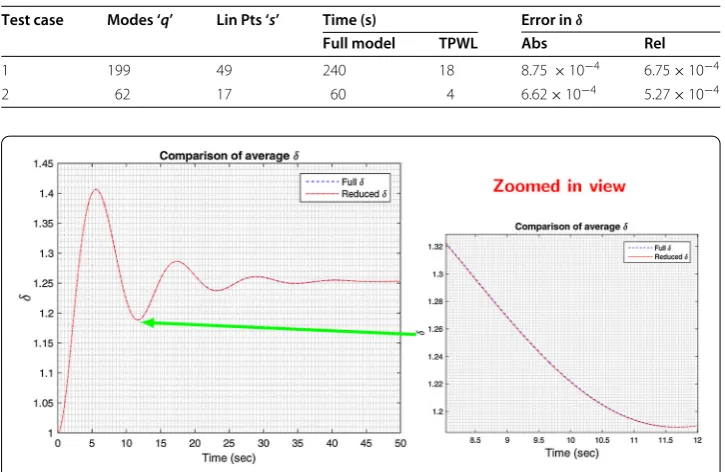
The results are very promising and the TPWL simulation is considerably faster as the full simulation in a similar case takes about 240 s while the TPWL simulation took about
Table 4 Time consumption data
Training trajectory Modes ‘q’ Lin Pts ‘s’ Time (s)
Full model POD Lin Pts Sel
Table 5 Initial conditions for test cases
Test cases δ2 δi ∀i=2
Test case 1 1.12 1
Test case 2 1.15 1.15
18 s with good accuracy. The errors are listed in the Table 6. The comparison of the averageδbetween the original and reduced order models are presented in Fig.4.
Second test case: synchronous non-equilibrium
This is a case similar to the third training trajectory where we had all the nodes starting from a synchronous non-equilibrium position, in this case we gave the initial conditions of 1.15 rather than 0.8 in the training caseδi=1.15∀i. The initial conditions used for this
test case are presented in Table5.
The results are excellent and the TPWL simulation is considerably faster as the full simulation in this case takes about 60 s while the TPWL simulation takes about 4 s with very high accuracy. The errors are listed in the Table6and the comparison of the average δbetween the original and reduced order models are presented in Fig.5.
Convergence analysis
It is important to analyse the source of error in the current study. As the results from the previous section shows that the error is small but not small enough as to compare with the machine precision level. In order to understand how does the error diminish and its dependency on various factors, we studied different factors namely, the number of modes, number of linearization points and the time step size. It is evident from the previous tables that the number of modes used has a little impact on error but considerable one on time
Table 6 Test cases of TPWL simulations
Test case Modes ‘q’ Lin Pts ‘s’ Time (s) Error inδ
Full model TPWL Abs Rel
1 199 49 240 18 8.75×10⁻⁴ 6.75×10⁻⁴
2 62 17 60 4 6.62×10⁻⁴ 5.27×10⁻⁴
Fig. 5 Comparison of the averageδfor the 2nd test case
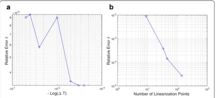
consumption during the simulation. The behavior of the maximum relative error in the reduced linearized variableδwith respect to the time step and the number of linearization points is shown in the Fig.6a and b , respectively. The non-monotonic behavior of the relative error as a function of time step in Fig.6a is due to the fact that for a larger time step compared to the one adopted for the training trajectory ( T = 0.005) the reduced order model might skip some of the linearization points. Hence, it is inferred that the time step used for the reduced model simulation should be at least equal to the time step used in the training simulation. For smaller time steps the error is bounded by the truncation error of the reduced basis.
It can be conclusively said that the major impact on the accuracy of the reduced order linearized model depends on having more linearized point. This is quite intuitive, since adding more points around which the linearization of the non-linear function is performed it will be able to capture the non-linear behavior more effectively and hence reducing the error.
Confidence interval
In order to give an idea of how the reduced model generated using TPWL compares with the high fidelity model, we carried out a simple analysis similar to sensitivity analysis. For this analysis, all the parameters were kept constant bar one. This is repeated for all the parameters. This analysis is performed using reduced basis generated using one training trajectory. The details of the training trajectory are similar to as listed in Table 1 and the initial values of the phase angles are listed in Table7. The number of linearization points (s) in the reduced basis for this case is 205 and the modes (q) selected are 199 out of 1000.
In Table 8 we presented the upper limit and the lower limit wherever applicable that we can use with confidence having a maximum relative error in {δ} of 5% or less. Due to the nature of the problem, the lower limit in the case of pm and upper limit of d are open-ended as the error is always bounded on these limits. The num-ber of generators N and the susceptancesbare not included in this exercise because they depend upon the network topology and changes in these will have to be incor-porated through a new reduced model. The mass of the generator is also not included since the equation is always normalized with the mass of the generator such thatmi is
one. The variation in the phase angle δ2 depends upon the initial condition, the per-formance of the reduced model simulation impvores with the inclusion of more than one training trajectory and hence, the range for δ2 increases from what is given in Table7.
As we have described earlier that in this method several training trajectories can be included in the offline phase to make the reduced basis. This implies that for values over the limits in the Table8, we can add another training trajectory so that the error remains acceptable.
Conclusions
TPWL proves to be a very robust method for model order reduction of models containing nonlinear functions. It has been proved as a fast, reliable and accurate MOR technique as observed from the results presented by the test cases in “Numerical experiments” section. The method as described is separated into offline and online phases, where in the offline phase the selection of linearization points is carried out. That is the only time consuming part of the method and as it is performed only once during offline phase the time penalty on the overall procedure is not severe.
Table 7 Initial conditions used in the build up for confidence interval
Trajectory for confidence interval δ2 δi ∀i=2
Trajectory 1 1.5 1
Table 8 Confidence interval for parameters with training trajectory of Table7
Parameter Upper limit Lower limit
pm 0.97 (p.u.) –
di – 0.15 (p.u.)
δ2 2.25 1
For the confidence interval, some other values of disturbances in{δ}, and different values ofpm, di, bintwere trialed and the results as shown in “Confidence interval” section proves
the robustness of the method considering the large variations possible for simulation with reduced model. Note that, the confidence interval’s simulation were performed with only one training trajectory and if more trajectories are included in the reduced basis the interval where the method can be applied increases and the results improves.
The method is very well adapted to the problem discussed in this study and more appli-cation for example, for the differential-algebraic equations (DAEs) of the network grids containing both generators (PV nodes) and the loads (PQ nodes), can further consolidate the current method as a well established model reduction method.
Authors’ contributions
All the authors contributed in the development and adaptation of the method for the current study. Malik performed the coding in MATLAB and drafted the manuscript. Borzacchielo, Diez and Chinesta supervised the study and advised on the draft and the corrections in the manuscript. All authors read and approved the final manuscript.
Author details
1Institut de Calcul Intensif (ICI), École Centrale de Nantes, 1 rue de la Noë, BP 92101, 44321 Nantes Cedex 3, France, 2Laboratori de càlcul numèric (LaCàN), Polytecnic University of Catalunya, C2 Campus Nord, Calle Jordi Girona, 31,
08034 Barcelona, Spain.
Competing interests
The authors declare that they have no competing interests.
Received: 18 July 2016 Accepted: 15 November 2016
References
1. Magnusson PC. The transient-energy method of calculating stability. Trans Am Inst Electr Eng. 1947;66(1):747–55. doi:10.1109/T-AIEE.1947.5059502.
2. Aylett PD. The energy-integral criterion of transient stability limits of power systems. Proc IEE Part C Monogr. 1958;105(8):527–36. doi:10.1049/pi-c.1958.0070.
3. Z. Bai PD, Freund R. Reduced-order modeling. In: Schilders EJWT, Maten W, editors. Handbook of numerical analysis Vol XIII, numerical methods in electromagnetics vol 13, 2nd edn. North Holland : Elsevier; 2005. p. 825–95. 4. Schilders W. Introduction to model order reduction. In: Schilders WHA, van der Vorst HA, Rommes J, editors. Model
order reduction: theory, research aspects and applications. Mathematics in industry, vol 13. Berlin: Springer; 2008. p. 3–32. doi:10.1007/978-3-540-78841-6.
5. Pinnau R. Model reduction via proper orthogonal decomposition. In: Schilders, WHA, van der Vorst HA, Rommes J, editors. Model order reduction: theory, research aspects and applications. Mathematics in industry, vol 13. Berlin: Springer; 2008. p. 95–109. doi:10.1007/978-3-540-78841-6.
6. Chinesta F, Leygue A, Bordeu F, Aguado JV, Cueto E, Gonzalez D, Alfaro I, Ammar A, Huerta A. Pgd-based computational vademecum for efficient design, optimization and control. Arch Comput Methods Eng. 2013;20(1):31–59. doi:10.1007/ s11831-013-9080-x.
7. Parrilo PA, Lall S, Paganini F, Verghese GC, Lesieutre BC, Marsden JE. Model reduction for analysis of cascading failures in power systems. In: American control conference, 1999. Proceedings of the 1999, vol 6. 1999. p. 4208–42126. doi:10. 1109/ACC.1999.786351.
8. Montier L, Henneron T, Clénet S, Goursaud B. Transient simulation of an electrical rotating machine achieved through model order reduction. Adv Model Simul Eng Sci. 2016;3(1):1–17. doi:10.1186/s40323-016-0062-z.
9. Kashyap N, Werner S, Riihonen T, Huang Y-F. Reduced-order synchrophasor-assisted state estimation for smart grids. In: Smart grid communications (SmartGridComm), 2012 IEEE third international conference. 2012. p. 605–10 . doi:10. 1109/SmartGridComm.2012.6486052.
10. Wille-Haussmann B, Link J, Wittwer C. Simulation study of a smart grid approach: Model reduction, reactive power control. In: Innovative smart grid technologies conference Europe (ISGT Europe), 2010 IEEE PES. 2010. p. 1–7. doi:10. 1109/ISGTEUROPE.2010.5638971.
11. Rewie ´nski MJ. A trajectory piecewise-linear approach to model order reduction of nonlinear dynamical systems. PhD thesis, Massachusetts Institute of Technology. 2003.
12. Liu Y, Yuan W, Chang H. A global maximum error controller-based method for linearization point selection in trajectory piecewise-linear model order reduction. IEEE Trans Comp Aided Des Integr Circuits Syst. 2014;33(7):1100–4. doi:10. 1109/TCAD.2014.2307000.
13. Chen Y, White J. A quadratic method for nonlinear model order reduction. In: Technical proceedings of the 2000 international conference on modeling and simulation of microsystems. 2000. p. 477–80.http://citeseerx.ist.psu.edu/ viewdoc/summary?doi=10.1.1.19.8951.
15. Qu L, Chapman PL. A trajectory piecewise-linear approach to model order reduction for nonlinear stationary magnetic devices. In: Computers in power electronics, 2004. Proceedings. 2004 IEEE workshop. 2004; p. 15–19. doi:10.1109/ CIPE.2004.1428113.
16. Rewienski M, White J. A trajectory piecewise-linear approach to model order reduction and fast simulation of nonlinear circuits and micromachined devices. IEEE Trans Comp Aided Des Integr Circuits Syst. 2003;22(2):155–70. doi:10.1109/ TCAD.2002.806601.
17. Farooq MU, Xia L, Hussin FAB, Malik AS. Automated model generation of analog circuits through modified trajectory piecewise linear approach with Chebyshev Newton interpolating polynomials. In: Intelligent systems modelling simulation (ISMS), 2013 4th international conference. 2013; p. 605–9. doi:10.1109/ISMS.2013.28.
18. Long C, Simonson LJ, Liao W, He L. Floorplanning optimization with trajectory piecewise-linear model for pipelined interconnects. In: Proceedings of the 41st annual design automation conference. 2004. p. 640–5.
19. Farooq MU, Xia L. Local approximation improvement of trajectory piecewise linear macromodels through chebyshev interpolating polynomials. In: Design automation conference (ASP-DAC), 2013 18th Asia and South Pacific. 2013. p. 767–72. doi:10.1109/ASPDAC.2013.6509693.
20. Burgard S, Farle O, Klis D, Dyczij-Edlinger R. Order-reduction of fields-level models with affine and non-affine parame-ters by interpolation of subspaces. IFAC PapersOnLine. 2015;48(1):170–5. doi:10.1016/j.ifacol.2015.05.111. 21. Panzer H, Mohring J, Eid R, Lohmann B. Parametric model order reduction by matrix interpolation.
Automatisierung-stechnik. 2010;58(8):475–84. doi:10.1524/auto.2010.0863.
22. Xie W, Theodoropoulos C. An off-line model reduction-based technique for on-line linear MPC applications for nonlinear large-scale distributed systems. In: Pierucci S, Ferraris GB, editors. In: 20th European symposium on computer aided process engineering. Computer aided chemical engineering, vol 28, . Amsterdam: Elsevier; 2010. p. 409–14. doi:10.1016/S1570-7946(10)28069-0.http://www.sciencedirect.com/science/article/pii/S1570794610280690. 23. He J, Sætrom J, Durlofsky LJ. Enhanced linearized reduced-order models for subsurface flow simulation. J Comput
Phys. 2011;230(23):8313–41. doi:10.1016/j.jcp.2011.06.007.
24. Cardoso MA, Durlofsky LJ. Linearized reduced-order models for subsurface flow simulation. J Comput Phys. 2010;229(3):681–700. doi:10.1016/j.jcp.2009.10.004.
25. Bergen AR, Vittal V. Power system analysis. 2nd ed. New Jersey: Prentice Hall; 1999.
26. Shampine LF, Reichelt MW. The MATLAB ODE suite. SIAM J Sci Comput. 1997;18:1–22. doi:10.1214/aoms/1177729959. 27. Liang YC, Lee HP, Lim SP, Lin WZ, Lee KH, Wu CG. Proper orthogonal decomposition and its applications—part I:
theory. J Sound Vib. 2002;252(3):527–44. doi:10.1006/jsvi.2001.4041.
28. Kerschen G, Golinval J-C, Vakakis AF, Bergman LA. The method of proper orthogonal decomposition for dynamical characterization and order reduction of mechanical systems: an overview. Nonlinear Dyn. 2005;41(1–3):147–69. doi:10. 1007/s11071-005-2803-2.
29. Berkooz G, Holmes P, Lumley JL. The proper orthogonal decomposition in the analysis of turbulent flows. Annu Rev Fluid Mech. 1993;25(1):539–75. doi:10.1146/annurev.fl.25.010193.002543.
30. Albunni MN. Model order reduction of moving nonlinear electromagnetic devices. PhD thesis, Technical University of Munich. 2010.
31. Rewienski M, White J. A trajectory piecewise-linear approach to model order reduction and fast simulation of nonlinear circuits and micromachined devices. In: Computer aided design, 2001. ICCAD 2001. In: IEEE/ACM international conference on. 2001. p. 252–7. doi:10.1109/ICCAD.2001.968627.
32. Acha E, Agelidis VG, Anaya-Lara O, Miller TJE. 4 - power flows in compensation and control studies. In: Acha E, Agelidis VG, Anaya-Lara O, Miller TJE, editors. Power electronic control in electrical systems. Newnes Power Engineering Series. Oxford: Newnes; 2002. p. 106–52. doi:10.1016/B978-075065126-4/50004-3.http://www.sciencedirect.com/ science/article/pii/B9780750651264500043.