Computer simulation of electron transport in solids with applications to materials analysis and characterization

(1)

Doctoral School in Materials Science and Engineering

XXV cycle

Computer simulation of electron transport in

solids with applications to materials analysis

and characterization

(2)

(3)

Computer simulation of electron transport in

solids with applications to materials analysis

and characterization

Maurizio Dapor

[email protected]

Approved by

:

Prof. S. Gialanella, Tutor,

University of Trento

PhD committee

:

Prof. P. Scardi,

University of Trento

Prof. S. Schmauder,

Universit¨

at Stuttgart

(4)

Doctoral Thesis

Maurizio Dapor - 2013

Published in Trento (Italy) by University of Trento

(5)

(6)

(7)

Acknowledgements

Firstly, I would like to gratefully thank my sweet wife, our beloved children, and my dear parents, for their immense patience, their generous availability, and their continuous support.

It is also a pleasure to mention many people, friends and colleagues, who, with their enthusiasm, invaluable suggestions, ideas, and competence, con-siderably contributed to achieve the results presented in this work.

I wish to express my warm gratitude to Diego Bisero, Lucia Calliari, Giovanni Garberoglio, and Simone Taioli, for their sincere friendship, encouragement, and excellent scientific suggestions.

I am particularly grateful to my tutor and advisor, Stefano Gialanella, for his patient guidance and continuous help.

I am also indebted with all the researchers who made possible with their help the completion of the project: Nicola Bazzanella, Eric Bosch, Mauro Ciappa, Michele Crivellari, Sergey Fanchenko, Wolfgang Fichtner, Massimiliano Fil-ippi, Stephan Holzer, Emre Ilg¨usatiroglu, Beverley J. Inkson, Mark A.E. Jepson, Alexander Koschik, Antonio Miotello, Cornelia Rodenburg, John M. Rodenburg, Manoranjan Sarkar, Giorgina Scarduelli, Stefano Simonucci, and Laura Toniutti.

I would like to thank all my colleagues at the Interdisciplinary Laboratory for Computational Science (LISC) in Trento for the fruitful discussions. The stimulating atmosphere of LISC provided the ideal environment to work to this project.

(8)

(9)

Monte Carlo and modeling methodology

61

5 Random numbers 63 5.1 Basic aspects . . . 63

5.1.1 Generating pseudo-random numbers . . . 63

5.1.2 Testing pseudo-random number generators . . . 64

5.1.3 Pseudo-random numbers distributed according to a given probability density . . . 65

5.2 Concluding remarks about random numbers . . . 67

6 Monte Carlo strategies 69 6.1 The continuous-slowing-down approximation . . . 70

6.1.1 The step-length . . . 70

6.1.2 Interface between over-layer and substrate . . . 71

6.1.3 The polar scattering angle . . . 71

6.1.4 Direction of the electron after the last deflection . . . . 73

6.1.5 The energy loss . . . 73

6.1.6 End of the trajectory and number of trajectories . . . . 74

6.2 The energy-straggling strategy . . . 74

6.2.1 The step-length . . . 74

6.2.2 Elastic and inelastic scattering . . . 75

6.2.3 Electron-electron collisions: scattering angle . . . 76

6.2.4 Electron-phonon collisions: scattering angle . . . 79

6.2.5 Direction of the electron after the last deflection . . . . 80

6.2.6 Transmission coefficient . . . 80

6.2.7 End of the trajectory and number of trajectories . . . . 83

(11)

CONTENTS 11

III

Experimental methods and materials

85

7 Experimental methods and materials 87

7.1 Backscattering coefficient of surface films . . . 87

7.1.1 Deposition of over-layer films . . . 87

7.1.2 Analysis of over-layer films . . . 88

7.2 Electron energy distribution spectra . . . 91

7.2.1 Reflection electron energy loss and Auger electron spectra 91 7.2.2 Secondary-electron emission spectra . . . 91

7.3 Materials . . . 92

7.4 Concluding remarks about experimental methods and materials 94

IV

Applications of the Monte Carlo method

95

8 Backscattering coefficient 97 8.1 Electrons backscatterd from bulk targets . . . 98

8.2 Electrons backscatterd from over-layers . . . 99

8.2.1 The experimental approach . . . 102

8.2.2 Thickness of contamination layers . . . 102

8.2.3 Possible source of uncertainties . . . 103

8.2.4 Thin films of palladium deposited on silicon . . . 105

8.2.5 Thin films of gold deposited on silicon . . . 106

8.2.6 Backscattered electrons from two layers deposited on semi-infinite substrates . . . 111

8.3 Concluding remarks about BSE . . . 112

9 Secondary electron yield 117 9.1 Secondary electron emission . . . 118

9.2 MC approaches to the study of SE emission . . . 119

9.3 Specific MC methodologies for SE studies . . . 119

9.3.1 Continuous-slowing-down approximation . . . 119

9.3.2 Energy-straggling . . . 120

9.4 Secondary electron yield: PMMA, SiO2, Al2O3 . . . 121

9.4.1 Comparison between ES scheme and experiment . . . . 122

9.4.2 Comparison between CSDA and ES schemes . . . 122

9.4.3 Comparison between CSDA scheme and experiment . . 123

(12)

9.4.5 CPU time . . . 129

9.5 Linewidth measurement in critical dimension SEM . . . 130

9.5.1 Nanometrology and linewidth measurement in CD SEM 130 9.5.2 Lateral and depth distributions . . . 132

9.5.3 Secondary electron yield as a function of the angle of incidence . . . 133

9.5.4 Linescan of a silicon step . . . 134

9.5.5 Linescan of PMMA lines on a silicon substrate . . . 135

9.6 Concluding remarks about secondary electron yield . . . 136

10 Electron energy distributions 139 10.1 Monte Carlo simulation of the spectrum . . . 140

10.2 Plasmon losses . . . 142

10.2.1 Plasmon losses in silicon dioxide . . . 142

10.2.2 Bulk and surface plasmon losses: Werner et al. ap-proximation . . . 144

10.2.3 Bulk and surface plasmon losses: Chen and Kwei theory148 10.3 Energy losses of Auger electrons . . . 158

10.4 Secondary electron spectrum . . . 160

10.4.1 Initial polar and azimuth angle of the SEs . . . 162

10.4.2 Comparison to theoretical and experimental data . . . 164

10.4.3 Application to energy selective scanning electron mi-croscopy . . . 167

10.5 Concluding remarks about energy distributions . . . 172

11 Conclusions 175

V

Appendices

177

A Mott theory 179

B Fr¨ohlich theory 185

C Ritchie theory 195

D Chen and Kwei theory 201

(13)

Chapter 1

Introduction

The interaction of electron beams with matter is a scientific topic that has interested many researchers since the first half of the twentieth century. In this regard, we can find in the literature many excellent works, among which the classic reviews of Bothe [1] and Birkhoff [2]. In the last decades several books and articles appeared, both experimental and theoretical, devoted to this subject: see, for example the works by Ibach [3], Niedrig [4], Goldsteinet al. [5], Newburyet al. [6], Feldman and Mayer [7], Sigmund [8], and Egerton [9, 10]. Many papers and books are dedicated specifically to transport Monte Carlo: among the numerous excellent works, see in particular the reviews by Carter and Cashwell [11], Salvat et al. [12], Shimizu and Ding Ze-Jun [13], Joy [14], and Bielajew [15].

1.1

Interaction of electrons with solid targets

In a typical experiment in which an electron beam impinges on a solid tar-get, many electrons of the primary electron beam can be backscattered, after having interacted with the atoms and electrons of the target. A fraction of them conserves the original kinetic energy, having experienced only elastic scattering collisions with the atoms of the target: these electrons constitute the elastic peak, whose maximum is located at the energy of the primary beam. Electrons scattered by electron-phonon collisions can be found very close to the elastic peak: their energy loss is typically lower than 0.1 eV. Electrons inelastically scattered by plasmon excitations can be found in a range of approximately 50 eV below the elastic peak. They represent the

(14)

electrons belonging to the primary electron beam that emerge from the sur-face after having suffered a single inelastic collision with a plasmon. Multiple collisions with plasmons are present in the spectrum as well: their intensities are quickly decreasing as the number of inelastic collisions increases. Elec-trons from direct ionization as well as Auger elecElec-trons can be found in the range from 50 eV to the energy of the elastic peak. The secondary elec-trons produced by a cascade process are those elecelec-trons which have been extracted from the atoms by inelastic electron-electron collisions and are able to emerge from the target surface. Their energy distribution presents a pronounced peak in the very low energy region of the spectrum, typically below 50 eV. The secondary electron emission yield is conventionally mea-sured integrating the area of the spectrum from 0 to 50 eV including, in such a way, also the tail of backscattered electrons. The number of backscattered electrons in this energy region is negligible and can be safely ignored unless the primary energy be very low as well.

1.2

Structure of the work

Monte Carlo (MC) technique allows solving mathematical and physical prob-lems of great complexity. One of the main topics that can be approached using the MC strategies concerns the study of the electron-solid interaction (transport MC). The aim of this work is to investigate some physical prob-lems related to the transport of electrons in solid targets using our transport MC codes. The numerical and theoretical results will be validated through a comparison with experimental evidences. We also tackle issues related to methodological aspects. In particular, we will make systematic comparisons among different calculation schemes. Different expressions for the calculation of cross sections and/or stopping power and different simulation methods will be compared with experimental data both acquired with specifically designed experiments – involving SEM, AES, and REELS – both taken from literature studies, in order to establish the limits of validity of the various theories and methods which have been proposed in the literature.

The thesis is divided in four parts.

(15)

theo-1.3. APPLICATIONS OF THE MC 15

retical calculations (by other authors) with the aim to validate the present approach.

The second part of the thesis is dedicated to the methodological aspects and, in particular, to the description of the present Monte Carlo method: we provide details, in particular, of the two MC schemes we have implemented in our code, i.e., the continuous-slowing-down approximation scheme (were electrons are assumed to continuously lose energy along their travel into the solid) and the energy-straggling approach (where the statistical fluctuations of the electron energy losses are properly taken into account).

The third part is devoted to a brief description of the experimental meth-ods: in this context, they are fundamental tools for the validation of the present MC calculations and for the comparison between the two MC schemes described in the second part. The materials used for the experiments and the MC simulations are also briefly described.

In the fourth part of the thesis, some critical aspects of the present MC approaches along with specific MC methodologies concerning particular phys-ical processes are discussed; comparison to experimental data are provided; and examples of technological applications are given.

In the appendices, the main theories utilized in our work for the calcu-lations of the various cross-sections are collected: they are the Mott theory of elastic scattering, the Fr¨ohlich theory of electron-phonon interaction, the Ritchie dielectric theory, and the Chen and Kwei theory of the depth depen-dence of the differential inverse inelastic mean free path. They are described there in order to make it easier and smoother the reading of the main text. Also a list of the papers published by the present author during his PhD course are provided in the last appendix.

1.3

Applications of the MC

(16)

(17)

Part I

Electron transport in solid

materials

(18)

(19)

Chapter 2

Electron transport in solids

The Monte Carlo method is used for evaluating the many physical quantities necessary to the study of the interactions of particle-beams with solid targets. The simulation of the relevant physical processes, by random sampling, allows to solve many particle transport problems. Considering the effects of the single collisions and letting the electrons carry out an artificial, random walk it is possible to accurately evaluate the diffusion process.

Studies of backscattered and secondary electrons are of great interest for many analytical techniques. A better comprehension of the processes which occur before the emission of backscattered and secondary electrons would allow a more general understanding of surface physics.

2.1

Electron-beam interactions with solids

During their travel in the solid, the incident electrons lose energy and change direction at each collision with the atoms bound in the solid. Because of the large difference between the masses of the electron and the atomic nu-cleus, nuclear collisions deflect electrons without any relevant kinetic energy transfer. This process is described by the differential elastic scattering cross-section (which can be calculated by the so-called relativistic partial wave expansion method, corresponding to the Mott cross-section [16]). The Mott cross-section can be approximated with the screened Rutherford formula: this is possible when the conditions corresponding to the first Born approx-imation are satisified, i.e., for high, even if not relativistic, energy and for low atomic number of the target atom. On the other hand, excitation and

(20)

ejection of atomic electrons, and excitation of plasmons, affect the energy dissipation. These processes only slightly affect the direction of the inci-dent electron in the solid, so that they can be described as inelastic events. Plasmon excitations are ruled by the equations for the differential inelastic scattering cross-sections, calculated by the use of Ritchie’s dielectric theory [17]. The Fr¨ohlich theory [18] can be used for describing the quasi-elastic electron-phonon interactions. Electron-phonon interactions are considered quasi-elastic for the corresponding energy losses and gains are very small when compared to the plasmon energy losses. When, in insulating materials, electron kinetic energies considerably decreases, trapping phenomena due to the polaronic effect have to be taken into account as well [19].

While for electron kinetic energies higher than 10 keV, MC simulations provide excellent results by the simple use of the Rutherford differential elastic scattering cross-section (elastic scattering) and of the Bethe-Bloch stopping power formula or semi-empirical stopping power formulas (inelastic scattering), when the electron energies become much lower than 5 keV – and this is the case of secondary electron emission – this approach fails. There are many reasons, and the most important ones are related to the three following facts:

(i) As the Rutherford formula is a result of the first Born approximation, it is a high energy approximation.

(ii) Also the Bethe-Bloch formula is valid only for quite high energies; in particular, the Bethe-Bloch stopping power does not provide the correct pre-dictions when the electron energyE becomes lower than the mean ionization energy J. It reaches a maximum for E ≈ 2.5J and then approaches zero as E approaches J/1.166. Below J/1.166, the predicted stopping power be-comes negative. The use of semi-empiric approaches can sometimes mitigate the problem. Actually, numerical approaches based on the calculation of the dielectric function - as a function of the energy loss and of the momentum transfer - are necessary to calculate low energy inelastic processes.

(21)

2.1. ELECTRON-BEAM INTERACTIONS WITH SOLIDS 21

the details of the energy loss mechanisms are not crucial for the accurate description of the process under investigation. CSDA can be used, for exam-ple, for the calculation of the backscattering coefficient. We will see that, in some specific cases, even the calculation of the secondary electron yield can be performed using CSDA. On the other hand, the description of the energy distributions of the emitted electrons (both backscattered and secondary) have to be performed avoiding the approximation of continuity in the energy loss processes and including energy straggling(ES) – i.e., the statistical fluc-tuations of the energy loss due to the different energy losses suffered by each electron of the penetrating beam – in the calculations.

A detailed approach able to accurately describe low energy elastic and inelastic scattering and to appropriately take into account the energy strag-gling is required for the description of secondary electron cascade. The whole cascade of secondary electrons must be followed: indeed any truncation, or cut off, underestimates the secondary electron emission yield. What is more, as already discussed, for insulating materials the main mechanisms of en-ergy loss cannot be limited to the electron-electron interaction for, when the electron energy becomes very small (lower than 10-20 eV, say), inelastic in-teractions with other particles or quasi-particles are responsible for electron energy losses. In particular, at very low electron energy, trapping phenomena due to electron-polaron interactions (polaronic effects) and electron-phonon interactions are the main mechanisms of electron energy loss. For the case of electron-phonon interaction, even phonon annihilations and the correspond-ing energy gains should be taken into account. Actually the energy gains are often neglected, for their probability of occurence is very small: much smaller, in any case, than the probability of phonon creation.

Summarizing, incident electrons are scattered and lose energy, due to the interactions with the atoms of the specimen, so that the incident electrons direction and kinetic energy are changed. It is usual to describe the collision events assuming that they belong to three distinct kinds: elastic (scatter-ing with atomic nuclei), quasi-elasic (scatter(scatter-ing with phonons) and inelastic (scattering with the atomic electrons and trapping due to polaronic effect).

2.1.1

Electron energy-loss peaks

(22)

31, 32, 33, 10, 9, 34, 35, 36]). An electron spectrum represents the number of electrons as a function of the energy they have after interaction with a target. The spectrum can be represented either as a function of the electron energy or of the energy-loss. In this second case, the first peak, centered at zero energy-loss, is known as the zero-loss peak. Also known as the elastic peak, it collects all the electrons which were transmitted – in transmission EELS (TEELS) – or backscattered – in reflection EELS (REELS) – without any measurable energy loss: it includes both the electrons which did not suffer any energy loss and those which were transmitted (TEELS) or backscattered (REELS) after one or more quasi-elastic collisions with phonons (for which the energy transferred is so small that, with conventional spectrometers, it cannot be experimentally resolved). In TEELS, elastic peak includes also all the electrons which were not scattered at all, namely which were not deflected during their travel inside the target and did not lose energy.

(23)

2.2. CHARACTERIZATION OF MATERIALS 23

100-200 eV from the elastic peak, in the energy spectrum).

For higher energy-losses, edges (of relatively low intensity with respect to the plasmon-losses), corresponding to inner-shell atomic electron excitations, can be observed in the spectrum. These edges are followed by slow falls, as the energy-loss increases. The energy position of these steps or, better, sharp rises, corresponds to the ionization threshold. The energy-loss of each edge is an approximate measure of the binding energy of the inner-shell energy level involved in the inelastic scattering process.

With an energy resolution better than 2 eV, it is possible to observe, in both the low-loss peaks and in the ionization threshold edges, detailed features related to the band structure of the target and its crystalline char-acteristics. For example, in carbon, plasmon peaks can be found at different energies in the spectrum, according to the carbon structure. This is due to the different valence-electron densities of diamonds, graphite and amorphous carbon.

For an excellent review about electron energy-loss spectra, see the Egerton book [10].

2.1.2

Secondary electron peak

Secondary electrons – produced by a cascade process – are those electrons extracted from the atoms by inelastic electron-electron collisions. Actually not all the secondary electrons generated in the solid emerge form the target. In order to emerge from the surface, the secondary electrons generated in the solid must reach the surface and satisfy given angular and energetic conditions. Of course, only the secondary electrons which are able to emerge from the target are included in the spectrum. Their energy distribution presents a pronounced peak in the region of the spectrum below 50 eV. The secondary electron emission yield is conventionally measured integrating the area of the spectrum from 0 to 50 eV (including, in such a way, also the tail of backscattered electron whose number, on the other hand, in this energy region is negligible – unless the primary energy be very low as well).

2.2

Characterization of materials

(24)

emission from solids irradiated by a particle beam is of crucial importance, especially in connection with the analytical techniques that utilize electrons to investigate chemical and compositional properties of solids in the near surface layers.

Electron spectroscopies and microscopies, examining how electrons inter-act with matter, represent fundamental tools to investigate electronic and optical properties of matter. The electron spectroscopies and microscopies allow to study the chemical composition, the electronic properties, and the crystalline structure of materials. According to the energy of the incident electrons, a broad range of spectroscopic techniques can be utilized: for ex-ample, Low Energy Electron Diffraction allows to investigate the crystalline structure of surfaces, Auger Electron Spectroscopy permits to analyze the chemical composition of the surfaces of solids, Electron Energy Loss Spec-troscopy – both in transmission, when the spectrometer is combined with Transmission Electron Microscope, and in reflection – can be used to char-acterize materials by comparing the shape of the plasmon-loss peaks and the fine-structure features due to interband and intraband transitions with those of suitable standards.

The study of the properties of a material using electron probes requires the knowledge of the physical processes corresponding to the interaction of the electrons with the particular material under investigation. A typical AES peak of an atomic spectrum, for example, has a width in the range from 0.1 to 1.0 eV. On the other hand, in a solid, many energy levels are involved which are very close in energy, so that broad peaks are typically observed in AES spectra of solids. Their features also depend on the instrumental resolution. Another important characteristic of the spectra is related to the shift in energy of the peaks due to chemical environment: indeed the core energy levels of an atom are shifted when it is a part of a solid. This property is used to characterize materials, as the shift can be determined theoretically or by comparison with suitable standards. Even the changes in spectral intensities and the appearence of secondary peaks can be used for analyzing unknown materials. Electron spectra are used for self-supported thin film local thickness measurements, multilayer surface thin film thickness evaluation, doping dose determination in semiconductors, radiation damage investigations, and so on.

(25)

2.3. CONCLUDING REMARKS ABOUT ELECTRON TRANSPORT 25

characterization through the study of the shape of plasmon-loss peaks [39]. Secondary electron investigation allows extraction of critical dimensions by modeling the physics of secondary electron image formation [40, 41, 42]. It permits to investigate doping contrast in p-n junctions and to evaluate accurate nanometrology for the most advanced CMOS processes [43, 44].

2.3

Concluding remarks about electron

trans-port

Transport Monte Carlo simulation is a very useful mathematical tool for describing many important processes relative to the interaction of electron beams with solid targets. In particular, the backscattered and secondary electron emission from solid materials can be investigated with the use of the Monte Carlo method. Many applications of the Monte Carlo study of backscattered and secondary electrons concern material analysis and charac-terization.

(26)

(27)

Chapter 3

Cross-sections: basic aspects

In the electron microscopies and spectroscopies, electrons penetrate into a material experiencing many different scattering processes. For a realistic description of the electron emission, it is necessary to know all the scattering mechanisms involved.

This chapter is devoted to the introduction of the concepts of cross-section and stopping power. For an excellent review of the topics treated in this chapter, also see Ref. [8]. The chosen approach is deliberately elementary, since the focus is on the basic aspects of the penetration theory. Specific details will be provided in the next chapter.

From the macroscopic point of view, thecross-sectionrepresents the area of a target that can be hit by a projectile, so that it depends on the geomet-rical properties of both the target and the projectile. Let us consider, for example, a point bullet impinging on a spherical target whose radius is r. The cross-section σ of the target is, in such a case, simply given byσ =πr2_.

In the microscopic world the concept has to be generalized in order to take into account that the cross-section does not only depend on the projec-tile and on the target, but also on their relative velocity and on the phys-ical phenonomena we are interested in: examples are represented by the

elastic scattering cross-section and the inelastic scattering cross-section of electrons (projectiles) impinging on atoms (targets). The elastic scattering cross-section describes the interactions in which the kinetic energy of the incident particle (the electron) does not change and is as a consequence the same before and after the interaction. The inelastic scattering cross-section, on the other hand, describes the collisions corresponding to an energy trans-fer from the incident particle (the electron) to the target (the atom): as a

(28)

consequence the kinetic energy of the incident electron decreases due to the interaction, so that the electron slows down. As the cross-section is a function of the kinetic energy of the incident electron, after every inelastic collision the cross-sections (both elastic and inelastic) of the subsequent collision, if any, will be accordingly changed.

In real experiments, the investigators cannot measure the cross-section corresponding to a single electron which hits a single atom. The typical experiment consists, instead, in the collision of a great number of electrons, called thebeam, with a medium constituted by a configuration of many atoms and/or molecules (a gas, for example, or an amorphous or crystalline solid). The electrons constituting the beam have, in principle, all the same initial energy (the primary energy) and do not interact with each other but only with the atoms of the medium. Actually, in practical cases, the energies of the electrons constituting the primary beam are distributed around the primary energy which has to be considered, as a consequence, their mean energy. Furthermore the electrons of the beam do not interact only with the target atoms (or molecules) but with each other as well. Neglecting these interactions corresponds to investigate the so-called low current beam approximation [8].

3.1

Cross-section and probability of

scatter-ing

Let us indicate withσthe cross-section of the physical effect we are interested in describing, and with J the density current, i.e., the number of electrons per unit area and per unit time in the beam. Let us indicate, furthermore, with N the number of target atoms per unit volume in the target and with

S the area of the target where the beam is spread. Let us assume that the beam spreading is homogeneous. Ifz is the depth where the collisions occur, then the volume where the electrons interact with the stopping medium is given by zS and, as a consequence, the number of collisions per unit time can be calculated by N zSJ σ. As the product of S by J is the number of electrons per unit time, the quantity

(29)

3.1. CROSS-SECTION AND PROBABILITY OF SCATTERING 29

represents the mean number of collisions per electron. In the hypothesis that the target thickness z is very small (thin layers) or the density of the target atoms N is very small (gas targets), so thatP 1, P represents the probability that an electron suffers a collision while travelling in the medium. In order to take into account that in the great majority of the experiments the projectile undergoes many collisions, let us associate to the trajectory of each particle a cylindrical volume V = zσ and calculate the probability Pν to hit ν target particles in this volume. If the positions of any two targets particle are not correlated like in the case, for example, of an ideal gas, such a probability is given by the Poisson distribution

Pν =

(N V)ν

ν! exp(−N V) =

(N zσ)ν

ν! exp(−N zσ), (3.2)

where ν = 0,1,2,3, ....

Let us firstly consider the single collision problem, ν = 1. The proba-bility of hiting precisely one particle in the volume zσ is given by

P1 = P(ν=1) = (N zσ) exp(−N zσ), (3.3)

so that, in the limit N zσ1,

P1 ∼= P = N zσ , (3.4)

which is the same result deduced above.

Also notice that, in the same limit, the probability for no collision at all is given by 1−P = 1−N zσ. This is the first order in N zσ of the well known Lambert and Beer’s absorption law:

P0 = P(ν=0) = exp(−N zσ). (3.5)

Note that, to the first order inN zσ, the probability for double events is equal to zero.

(30)

hνi = h(ν− hνi)2i = N zσ , (3.6) so that the relative fluctuation goes to zero as the reciprocal of the square root ofhνi = N zσ:

v u u t

h(ν− hνi)2_i

hνi2 =

1

√

ν . (3.7)

3.2

Stopping power and inelastic mean free

path

Let us now consider the collisions with the stopping medium resulting in a kinetic energy transfer from the projectile to the target atoms and/or molecules constituting the target. Let us assume that the energy transfersTi

(i = 1,2, ...) are small with respect to the incident particle kinetic energy

E. Let us also assume that νi be the number of events corresponding to the energy loss Ti, so that the total energy ∆E lost by an incident particle passing through a thin film of thickness ∆z is given by P

iνiTi.

As the mean number of collisions of typei, according to Eq. (3.6), is given byhνii = N∆zσi, where σi is the energy-loss cross-section, the energy loss is given by

h∆Ei = N∆zX

i

Tiσi . (3.8)

The stopping poweris defined as

h∆Ei

∆z = N

X i

Tiσi , (3.9)

and thestopping cross-section S is given by

S = X

i

Ti σi , (3.10)

(31)

3.3. RANGE 31

h∆Ei

∆z = N S . (3.11)

If the spectrum of the energy loss in continuous, instead of discrete, the

stopping cross-section assumes the form

S =

Z

T dσinel

dT dT , (3.12)

while the total inelastic scattering cross-section σinel is given by

σinel =

Z dσ

inel

dT dT , (3.13)

and dσinel/dT is the so-called differential inelastic scattering cross-section.

Once the total inelastic scattering cross-section σinel is known, the inelastic

mean free path λinel can be calculated by

λinel =

1

N σinel

. (3.14)

3.3

Range

While the inelastic mean free path is the average distance between two inelas-tic collisions, the maximum range is the total path length of the projectile. It can be easily estimated – using the simple way we are describing in this section – in all the cases in which the energy straggling, i.e., the statistical fluctuations in energy loss, can be neglected because small. Indeed, in this case, the energy of the incident particle is a decreasing function of the depth

z calculated from the surface of the target, so that E = E(z). As the stop-ping cross-section is, on the other hand, a function of the incident particle energy, S = S(E), the equation (3.11) assumes the form of the following differential equation

dE

dz = −N S(E), (3.15)

(32)

as already noticed, the projectile energyE(z) is a decreasing function of the depthz. Indicating withE0 the initial energy of the projectiles (the so-called

beam primary energy) the maximum range R can be easily obtained by the integration

R =

Z R

0

dz =

Z 0

E0

dE dz

dE , (3.16)

so that

R =

Z E0

0

dE

N S(E) . (3.17)

3.4

Energy straggling

Actually the range calculated in such a way can be different from the real one because of the statistical fluctuations of the energy loss. The consequences of such a phenomenon, known as energy straggling, can be evaluated following a procedure similar to that used for introducing the stopping cross-section.

Let us firstly consider then, as before, the discrete case and calculate the variance Ω2, or mean square fluctuation, in the energy loss ∆E, given by

Ω2 = h(∆E − h∆Ei)2i. (3.18)

Since

∆E − h∆Ei = X i

(νi− hνii)Ti , (3.19)

we have, due to the statistical independence of the collisions and the prop-erties of the Poisson distribution,

Ω2 = X

i

h(νi− hνii)2iTi2 = X

i

hniiTi2 . (3.20) As a consequence, taking into account that hnii = N∆zσi, the energy straggling can be expressed as

Ω2 = N ∆z X

i

(33)

3.5. CONCLUDING REMARKS ABOUT CROSS-SECTIONS 33

where we have introduced the straggling parameter defined as

W = X

i

T_i2 σi . (3.22)

If the spectrum of the energy loss is continuous, instead of discrete, the straggling parameter assumes the form

W =

Z

T2 dσinel

dT dT . (3.23)

3.5

Concluding remarks about cross-sections

(34)

(35)

Chapter 4

Scattering mechanisms

This chapter is devoted to the main mechanisms of scattering (elastic, quasi-elastic, and inelastic) which are relevant for the description of the interaction of electron beams with solid targets.

We shall firstly describe the elastic scattering cross-section, comparing the screened Rutherford formula to the more accurate Mott cross-section [16]. The Mott theory is based on the relativistic partial wave expansion method and the numerical solution of the Dirac equation in a central field. We shall show that the Mott cross-section is in better agreement with the available experimental data.

Then we shall briefly describe the Fr¨ohlich theory as well [18], which describes the quasi-elastic events occurring when electron energy is very low and the probability of electron-phonon interaction becomes significant. We shall discuss energy loss and energy gain due to electron phonon-interactions, and see that electron energy gains can be safely neglected, while electron energy losses are fractions of eV.

The Bethe stopping power [45] and semi-empiric approaches [46, 47] will be presented, along with the limits of these models for the calculation of energy losses.

The Ritchie dielectric theory [17] will be then considered, which is used for the accurate calculation of electron energy losses due to electron-plasmon interaction.

Polaronic effect will be also mentioned, as it is an important mechanism for trapping very slow electrons in insulating materials [19].

In the end of the chapter, a discussion about the inelastic mean free path will be provided which takes into account all the inelastic scattering

(36)

mechanisms introduced in this chapter.

Many details about the most important theoretical models presented in this chapter can be found in the relative Appendices.

4.1

Elastic scattering

Electron-atom elastic scattering is the main responsible for the angle deflec-tion of electrons traveling in solid targets. For some excellent reviews about the subject of elastic scattering see, for example, Refs. [8, 10, 9, 48].

Elastic scattering is not only the cause of the electron deflection: it has to be taken into account also for electron energy-loss problems, for it contributes in changing the angular distribution of the inelastically scattered electrons [10, 9].

Since a nucleus is much more massive that an electron, the energy transfer is usually negligible in an electron-nucleus collision. The great majority of elastic collisions correspond to the interaction of the incident electrons with the electrostatic nuclear field in regions which are far from the center of mass of the nucleus where, due to both the inverse square law and the shielding of the nucleus by the atomic electrons, the potential is relatively weak. For this reason, many electrons are elastically scattered through small angles.

Conservation of energy and momentum requires small transfers of energy between the electrons and the nuclei which depends on the angle of scat-tering. Even if the electron energy transfers are very small fraction of eV, in many circumstances they cannot be neglected. Furthermore notice that, despite to this general rule, in a few cases significant energy transfers are possible. Indeed, even if electron energy-losses are typically very small and often ignorable in electron-nucleus collisions, for the very rare cases of head-on collisihead-ons, where the scattering angle is equal to 180◦, the energy transfer can be, for the case of light elements, higher than the displacement energy, namely the energy necessary to displace the atom from its lattice position. In these cases, displacement damage and/or atom removal (sputtering) can be observed [10, 9].

The differential elastic scattering cross-section represents the probability per unit solid angle that an electron be elastically scattered by an atom, and is given by the square modulus of the complex scattering amplitude

(37)

4.1. ELASTIC SCATTERING 37

distribution, once taken into account that the Coulomb potential is screened by the atomic electrons, can be calculated either by the use of the first Born approximation (screened Rutherford cross-section) or, to get more accurate results – in particular for low-energy electrons –, by solving the Schr¨odinger equation in a central field (partial wave expansion method, PWEM).

Typically, for the case of the screened Rutherford formula obtained within the first Born approximation, the screening of atomic electrons is treated using the Wentzel formula [49], which corresponds to a Yukawa exponential attenuation of the nuclear potential as a function of the distance from the center of mass of the nucleus. The more accurate partial wave expansion method requires a better description of the screening, so that Dirac-Hartree-Fock-Slater methods are generally used for calculating the screened nuclear potential in this case.

A further improved approach to get a very accurate calculation of the differential elastic scattering cross-section, valid also for relativistic electrons, is represented by the so-called relativistic partial wave expansion method (RPWEM), – which is based on the solution of the Dirac equation in a central field (Mott cross-section) – where the sum of the squares of the moduli of two complex scattering amplitudes f and g is required for the calculation of the elastic scattering probabilities [16]. Also in this case, Dirac-Hartree-Fock-Slater methods are utilized to calculate the shielded nuclear potential.

4.1.1

Mott section vs. screened Rutherford

cross-section

The relativistic partial wave expansion method (Mott theory) [16] permits to calculate the differential elastic scattering cross-section as follows:

dσel

dΩ =|f |

2 ₊_|_g _|2 _, _(4.1)

where f(ϑ) and g(ϑ) are the scattering amplitudes (direct and spin-flip, re-spectively). For details about the Mott theory, see appendix A [34, 35, 36].

Once calculated the differential elastic scattering cross-section, the total elastic scattering cross-section σel and the first transport elastic scattering

cross-section σtr can be computed using the following equations:

σel =

Z dσ

el

(38)

σtr =

Z

(1−cosϑ) dσel

dΩ dΩ, (4.3)

It can be interesting to investigate the high energy and low atomic number limits of the Mott theory (corresponding to the first Born approximation). Along with the assumption that the atomic potential can be written accord-ing to the Wentzel recipe [49]:

V(r) = Z e

2

r exp

−r

a

, (4.4)

wherer is the distance between the incident electron and the nucleus,Z the target atomic number,ethe electron charge, andaapproximately represents the screening of the nucleus by the orbital electrons, given by

a = a0

Z1/3 , (4.5)

where a0 is the Bohr radius, the first Born approximation permits to write

the differential elastic scattering cross-section in an analytic closed form. It is the so-called screened Rutherford cross-section:

dσel

dΩ =

Z2e4

4E2

1

(1 − cosθ + α)2 , (4.6)

α = me

4_π2

h2

Z2/3

E (4.7)

(39)

4.1. ELASTIC SCATTERING 39

Rutherford theories – are compared. The presented data concern two differ-ent elemdiffer-ents (Cu and Au) and energies (1000 eV and 3000 eV). It is quite clear by the comparison that the Rutherford theory approaches the Mott theory as the atomic number decreases and the primary energy increases. Indeed, the Rutherford formula can be deduced assuming the first Born ap-proximation, which is valid when

E e

2

2a0

Z2 . (4.8)

In other words, higher the electron energy – in comparison with the atomic potential – higher the accuracy of the Rutherford theory (see, in particular, Fig. 4.3). Anyway, the Rutherford formula represents a decreasing function of the scattering angle, so that it should not be surprising that it cannot describe the features which emerges as the electron energy is low and atomic number is high (see, in particular, Fig. 4.2).

0 2 0 4 0 6 0 8 0 1 0 0 1 2 0 1 4 0 1 6 0 1 8 0 0 . 0 1

0 . 1

1

1 0

D

E

S

C

S

(

Å

2 /s

r)

S c a t t e r i n g a n g l e ( d e g )

Figure 4.1: Present calculation of the differential elastic scattering cross-section of 1000 eV electrons scattered by Cu as a function of the scattering angle. Solid line: Relativistic partial wave expansion method (Mott theory). Dashed line: Screened Rutherford formula, Eq. (4.6).

(40)

0 2 0 4 0 6 0 8 0 1 0 0 1 2 0 1 4 0 1 6 0 1 8 0 1 E - 3

0 . 0 1 0 . 1

1

1 0

D

E

S

C

S

(

Å

2/s

r)

Figure 4.2: Present calculation of the differential elastic scattering cross-section of 1000 eV electrons scattered by Au as a function of the scattering angle. Solid line: Relativistic partial wave expansion method (Mott theory). Dashed line: Screened Rutherford formula, Eq. (4.6).

accurate Mott cross-section – mainly because it provides a very simple an-alytic way to calculate both the cumulative probability of elastic scattering into an angular range from 0 toθ, Pel(θ, E), and the elastic scattering mean

free path,λel. Even if not used in this work, where numerical calculations of

Mott cross-section will always be utilized, it can be useful to see howPel(θ, E)

and λel can be calculated in a completely analytic way taking advantage of

the particular form of the screened Rutherford formula. In the first Born approximation these quantities are in fact given, respectively, by

Pel(θ, E) =

(1 + α/2) (1 − cosθ)

1 + α − cosθ , (4.9)

λel =

α(2 + α)E2

N π e4 _Z2 , (4.10)

(41)

4.1. ELASTIC SCATTERING 41

0 2 0 4 0 6 0 8 0 1 0 0 1 2 0 1 4 0 1 6 0 1 8 0 1 E - 3

0 . 0 1 0 . 1

1 1 0 D E S C S ( Å 2 /s r)

Figure 4.3: Present calculation of the differential elastic scattering cross-section of 3000 eV electrons scattered by Cu as a function of the scattering angle. Solid line: Relativistic partial wave expansion method (Mott theory). Dashed line: Screened Rutherford formula, Eq. (4.6).

The demonstration of these equations is quite easy. Indeed

Pel(θ, E) =

e4_Z2

4σelE2

Z θ

0

2πsinϑ dϑ

(1 − cosϑ + α)2 =

πe4_Z2

2σelE2

Z 1−cosθ+α α

du

u2 ,

where

σel =

e4_Z2

4E2

Z π

0

2πsinϑ dϑ

(1 − cosϑ + α)2 =

πe4_Z2

2E2

Z 2+α α

du

u2 .

Since

Z 1−cosθ+α α

du

u2 =

1−cosθ

α(1−cosθ+α)

(42)

0 2 0 4 0 6 0 8 0 1 0 0 1 2 0 1 4 0 1 6 0 1 8 0 1 E - 3

0 . 0 1 0 . 1

1

1 0

D

E

S

C

S

(

Å

2/s

r)

Figure 4.4: Present calculation of the differential elastic scattering cross-section of 3000 eV electrons scattered by Au as a function of the scattering angle. Solid line: Relativistic partial wave expansion method (Mott theory). Dashed line: Screened Rutherford formula, Eq. (4.6).

Z 2+α α

du

u2 =

1

α(1 +α/2) ,

Eqs. (4.9) and (4.10) immediately follow.

Note that from the cumulative probability expressed by Eq. (4.9) it follows that the scattering angle can be easily calculated from:

cosθ = 1 − 2α Pel(θ, E)

2 + α − 2Pel(θ, E)

. (4.11)

(43)

4.2. QUASI-ELASTIC SCATTERING 43

0 2 0 4 0 6 0 8 0 1 0 0 1 2 0 1 4 0 1 6 0 1 8 0 1 E - 3

0 . 0 1 0 . 1

1

1 0

D

E

S

C

S

(

Å

2 /s

r)

Figure 4.5: Present calculation of the differential elastic scattering cross-section of 1100 eV electrons scattered by Au as a function of the scattering angle. Solid line: Relativistic partial wave expansion method (Mott theory). Circles: Reichert experimental data [50].

the simple screened Rutherford formula, Eq. (4.6), provided that the kinetic primary energy of the incident electrons is higher than 10 keV.

4.2

Quasi-elastic scattering

Due to thermal excitations, atoms in crystalline structures vibrate around their equilibrium lattice sites. These vibrations are known as phonons. A mechanism of energy loss (and energy gain as well) is represented by the interaction of the electrons with the optical modes of the lattice vibrations. These transfers of small amounts of energy among electrons and lattice vibra-tions are due to quasi-elastic processes known as phonon creation (electron energy-loss) and phonon annihilation(electron energy-gain) [18, 51]. Phonon energies do not exceed kBTD, where kB is the Boltzmann constant and TD

is the Debye temperature. As kBTD typically is not greater than 0.1 eV,

(44)

much smaller probability, energy gain – are particularly relevant when the electron energy is low (few eV) [19].

4.2.1

Electron-phonon interaction

According to Fr¨ohlich [18] and Llacer and Garwin [51], the inverse mean free path for electron energy loss due to phonon creation can be written as

λ−_phonon1 = 1

a0

ε0 − ε∞

ε0 ε∞

¯

hω E

n(T) + 1

2 ln

 

1 + q1 − ¯hω/E

1 − q1 − ¯hω/E



 , (4.12)

whereE is the energy of the incident electron,Wph = ¯hω the electron energy

loss (of the order of 0.1 eV), ε0 the static dielectric constant, ε∞ the high

frequency dielectric constant, a0 the Bohr radius and

n(T) = 1

e¯hω/kBT − 1 (4.13)

the occupation number. Notice that a similar equation can be written to describe electron energy gain (corresponding to phonon annihilation). The probability of occurrence of phonon annihilation is much lower than that of phonon creation. Electron energy gain can thus be safely neglected for many practical purposes.

For further details about electron-phonon interaction and Fr¨ohlich theory [18, 51] see Appendix B.

4.3

Inelastic scattering

Let us consider now the inelastic scattering due to the interaction of the inci-dent electrons with the atomic electrons located around the nucleus (both the core and the valence electrons). For an excellent review about this subject, see Ref. [10].

If the incident electron energy is high enough, it can excite an inner-shell

(45)

4.3. INELASTIC SCATTERING 45

and its ground state; while the atom is left in an ionized state. The follow-ing de-excitation of the target atom generates an excess energy that can be liberated in one of two competitive ways: either generating an X-ray photon (Energy Dispersive Spectroscopy, EDS, is based on this process) or by the emission of another electron (Auger emission): this is the phenomenon on which Auger Electron Spectroscopy is based.

Outer-shell inelastic scattering can occur according to two alternative processes. In the first one, an outer-shell electron can suffer a single-electron excitation. A typical example is constituted by inter-band and intra-band transitions. If the atomic electron excited in such a way is able to reach the surface with an energy higher than the potential barrier between the vacuum level and the minimum of the conduction band, it can emerge from the solid as a secondary electron, the energy needed for this transition being provided by the fast incident electron. De-excitation can occur through the emission of electromagnetic radiation in the visible region – corresponding to the phenomenon known as cathode-luminescence – or through radiation-less processes generating heat. Outer-shell electrons can also be excited in collec-tive states corresponding to the oscillation of the valence electrons denoted as plasma resonance. It is generally described as the creation of quasi-particles known as plasmons, with energies – characteristic of the material – that range, typically, in the interval from 5 to 30 eV. Plasmon decay generates secondary electrons and/or produces heat.

4.3.1

Stopping: Bethe-Bloch formula

In the CSDA, energy losses are calculated by utilizing the stopping power. Using a quantum mechanical treatment, Bethe [45] proposed the following formula for the stopping power:

−dE

dz =

2πe4_{N Z}

E ln

₁_.₁₆₆_E

I

, (4.14)

where I represents the mean ionization energy which, according to Berger and Seltzer [52], can be approximated by the following simple formula:

(46)

higher than ∼ I. It approaches zero as E approaches I/1.166. When E

becomes smaller than I/1.166, the stopping power predicted by the Bethe-Bloch formula becomes negative. Therefore, the low-energy stopping power requires a different approach (see the dielectric approach, below).

4.3.2

Stopping: semi-empiric formulas

The stopping power can also be described using semi-empiric expressions, such as the following;

−dE

dz =

KeN Z8/9

E2/3 , (4.16)

proposed in 1972 by Kanaya and Okayama (withKe = 360 eV5/3 ˚A2) [47].

This last formula allows one to analytically evaluate the maximum range of penetration as a function of the primary energy E0, where

R=

Z 0

E0

dE

dE/dz =

3E₀5/3

5KeN Z8/9

∝ E₀1.67. (4.17)

A similar empirical formula for the evaluation of the maximum range of penetration of electrons in solid targets was firstly proposed, in 1954, by Lane and Zaffarano [46] who found that their range-energy experimental data (obtained by investigating electron transmission in the energy range 0-40 keV by thin plastic and metal films) fell within 15 percent of the results obtained by the following simple formula:

E0 = 22.2R0.6 , (4.18)

where E0 was expressed in keV and R in mg/cm2. As a consequence, the

Kanaya and Okayama formula is consistent with the Lane and Zaffarano experimental observations, which are described as well by the relationship

(47)

4.3. INELASTIC SCATTERING 47

4.3.3

Dielectric theory

In order to get a very accurate description of the electron energy loss pro-cesses, of the stopping power, and of the inelastic mean free path, valid even when electron energy is low, it is necessary to consider the response of the en-semble of conduction electrons to the electromagnetic field generated by the electrons passing through the solid: this response is described by a complex dielectric function. In the Appendix C the Ritchie theory [17, 20] is described which demonstrates, in particular, that the energy loss function,f(k, ω), nec-essary to calculate both the stopping power and the inelastic mean free path, is the reciprocal of the imaginary part of the dielectric function

f(k, ω) = Im "

1

ε(k, ω)

#

. (4.20)

In Eq. (4.20), ¯h~k represents the momentum transferred and ¯hω the electron energy loss.

Once known the energy loss function, the differential inverse inelastic mean free path can be calculated as [26]

dλ−_inel1

dhω¯ =

1

π E a0

Z k+

k−

dk

k f(k, ω), (4.21)

where

¯

h k± =

√

2m E ± q2m(E − ¯hω), (4.22)

E is the electron energy, m the electron mass, anda0 the Bohr radius. The

limits of integration, expressed by Eq. (4.22), come from conservation laws (see section 6.2.3).

In order to calculate the dielectric function, and hence the energy loss-function, let us consider the electric displacement D~ [35, 36]. If P~ is the polarization density of the material, and E~ the electric field, then

~

P = χεE~, (4.23)

(48)

χε =

ε − 1

4π (4.24)

and

~

D = E~ + 4 π ~P = (1 + 4πχε)E~ = ε ~E . (4.25)

Ifn is the density of the outher-shell electrons, i.e., the number of outer-shell electrons per unit volume in the solid, and ξ the electron displacement due to the electric field, then

P = e n ξ , (4.26)

so that

|E|~ = 4π e n ξ

ε − 1 . (4.27)

Let us consider the classical model of electrons elastically bound, with elastic constants kn = mω2n and subject to a frictional damping effect due to

colli-sions, irradiations, described by a damping constant Γ. We have indicated here with m the electron mass and with ωn the natural frequencies. The

electron displacement satisfies the equation [22]

m ξ¨ + βξ˙ + k ξ = eE (4.28)

where β =mΓ. Assuming that ξ = ξ0 exp(iωt), a straightforward

calcula-tion allows to conclude that

ε(0, ω) = 1 − ω

2 p

ω2 ₋ _ω2

n − iΓω

, (4.29)

whereωp is the plasma frequency, given by

ω_p2 = 4π n e

2

(49)

4.3. INELASTIC SCATTERING 49

Let us now consider a superimposition of free and bound oscillators. In such a case the dielectric function can be written as:

ε(0, ω) = 1 − ω_p2 X

n

fn

ω2 ₋ _ω2

n − iΓnω

, (4.31)

where Γn are positive frictional damping coefficients and fn are the fractions

of the valence electrons bound with energies ¯hωn.

The extension of the dielectric function from the optical limit (corre-sponding to k = 0) to k > 0 is obtained including, in the previous formula, an energy ¯hωk related to the dispersion relation, so that

ε(k, ω) = 1 − ω_p2 X

n

fn

ω2 ₋ _ω2

n − ω2k − iΓnω

. (4.32)

In the determination of the dispersion relation, one has to take into account a constraint, known as the Bethe ridge. According to the Bethe ridge, as

k → ∞, ¯hωk should approach ¯h2k2/2m. Of course, an obvious way to obtain this result (the simplest one, actually) is to impose that [26, 29],

¯

hωk =

¯

h2k2

2m . (4.33)

Another way to satisfy the constraint represented by the Bethe ridge corre-sponds to the use of the following equation [17, 20]:

¯

h2 ω2_k = 3 ¯h

2 _v2

F k2

5 +

¯

h4 k4

4m2 , (4.34)

where vF represents the velocity of Fermi.

Once the dielectric function is known, the loss function Imh_ε₍_k,ω1 ₎iis given by

Im "

1

ε(k, ω)

#

= − ε2

ε2

1+ε22

, (4.35)

(50)

ε(k, ω) = ε1(k, ω) +iε2(k, ω), (4.36)

The calculation of the energy loss function can be also performed by the direct use of experimental optical data. In Figs. 4.6 and 4.7, the energy loss function of Polymethyl Methacrylate and silicon dioxide are represented, respectively. The calculation of the dielectric function from optical data can be performed by

ε1(0, ω) =µ2−ν2 , (4.37)

ε2(0, ω) =−2µν (4.38)

whereµ is the index of refraction and ν the extinction coefficient.

1 1 0 1 0 0 1 0 0 0 1 0 0 0 0

1 E - 9 1 E - 8 1 E - 7 1 E - 6 1 E - 5 1 E - 4 1 E - 3 0 . 0 1 0 . 1

1

1 0

E

n

e

rg

y

l

o

s

f

u

n

c

ti

o

n

E n e r g y t r a n s f e r ( e V )

Figure 4.6: Optical energy loss function for electrons in Polymethyl Methacrylate. For energies lower than 72 eV we utilized the optical data of Ritsko et al. [53]. For higher energies the calculation of the optical loss function was performed using the Henkeet al. atomic photo-absorption data [54, 55].

(51)

4.3. INELASTIC SCATTERING 51

1 0 1 0 0 1 0 0 0

1 E - 6 1 E - 5 1 E - 4 1 E - 3 0 . 0 1 0 . 1

1 E n e rg y l o s s f u n c ti o n

E n e r g y t r a n s f e r ( e V )

Figure 4.7: Optical energy loss function for electrons in silicon dioxide (SiO2).

For energies lower than 33.6 eV we utilized the optical data of Buechner [56]. For higher energies the calculation of the optical loss function was performed using the Henke et al. atomic photo-absorption data [54, 55].

Im "

1

ε(k, ω)

# =

Z +∞

0

dω0 ω0 Im

" 1

ε(0, ω0₎

#

δ[¯h ω − (¯h ω0 + m k2/2)]

ω .

(4.39)

allows the extension of the dielectric function from the optical limit to k >0 [24, 25].

Penn [24] and Ashley [25] calculated the energy loss function using optcal data and extending as described above [see Eq. (4.39)] the dielectric function from the optical limit tok >0. According to Ashley [25], the inverse inelastic mean free path λ−_inel1 of electrons penetrating solid targets can be calculated by

λ−_inel1(E) = me

2

2π¯h2E

Z Wmax

0

Im "

1

ε(0, w)

#

L

_w

E

dw , (4.40)

where E is the incident electron energy and Wmax = E/2 (as usual, we

have indicated with e the electron charge and with ¯h the Planck constant

(52)

the momentum transfer ¯h~k was set to 0 and the ε dependence on ~k was factorised through the function L(w/E). Ashley [25] demonstrated that a good approximation of the function L(x) is given by:

L(x) = (1−x) ln 4

x −

7 4x+x

3/2₋33

32x

2 _. _(4.41)

The calculation of the stopping power, −dE/dz, can be performed by using the following equation [25]:

−dE

dz =

me2

π¯h2E

Z Wmax

0

Im "

1

ε(0, w)

#

S

w

E

w dw , (4.42)

where

S(x) = ln1.166

x −

3 4x−

x 4ln 4 x + 1 2x

3/2₋ x2

16ln 4

x −

31 48x

2 _. _(4.43)

In Figs. 4.8 and 4.9 the stopping power of electrons in PMMA and in SiO2

are, respectively, shown and compared with calculations perfromed by other authors. The present calculations were obtained using the just described Ashley recipe.

The differential inverse inelastic mean free path dλ−_inel1(w, E)/dw can be calculated using the following equation:

dλ−_inel1(w, E)

dw =

me2

2πh¯2EIm

" 1

ε(0, w)

# L _w E . (4.44)

Bulk and surface plasmon losses

The plasma frequencyωp is given, in the Drude free electron theory, by Eq.

(4.30) and represent the frequency of the volume collective excitations, which correspond to the propagation in the solid of bulk plasmons with energy

Ep = ¯hωp . (4.45)

(53)

4.3. INELASTIC SCATTERING 53

1 0 1 0 0 1 0 0 0 1 0 0 0 0

0

1

2

3

4

-d

E

/d

z

(

e

V

/

Å

)

E n e r g y ( e V )

Figure 4.8: Stopping power of electrons in PMMA. Solid line represents the present calculation, obtained according to the Ashley recipe [25]. Dashed line provides the Ashley original results [25]. Dotted line describes the Tan

et al. computational results [57]. The different optical energy loss functions utilized in the three cases explain the differences in the calculations.

1 0 0 1 0 0 0 1 0 0 0 0

0

1

2

3

4

-d

E

/d

z

(

e

V

/

Å

)

E n e r g y ( e V )

Figure 4.9: Stopping power of electrons in SiO2. Solid line represents the

(54)

plasmon peak whose maximum is located at an energy Ep [given by Eq.

(4.45)] from the elastic or zero-loss peak.

Also features due to surface plasmon excitations appear in spectra ac-quired either in reflection mode from bulk targets or in transmission mode from very thin samples or small particles [59]. Indeed, in the proximity of the surface, due to the Maxwell’s equation boundary conditions, surface ex-citations modes (surface plasmons) take place with a resonance frequency slightly lower than the bulk resonance frequency.

A rough evalution of the energy of the surface plasmons can be performed – for a free electron metal – by the following very simple considerations [10]. In general, similarly to the volume plasmons propagating inside the solid, in the presence of an interface between two different materials – which we indicate here with a and b –, longitudinal waves travel as well along the interface. From continuity considerations it follows that [10]

εa + εb = 0 , (4.46)

where we have indicated withεa the dielectric function on the sideaand with

εb the dielectric function on the sideb of the interface. Let us now consider

the particular case corresponding to a vacuum/metal interface and ignore, for the sake of simplicity, the damping, so that Γ≈0. Then, if a represents the vacuum, we get

εa = 1, (4.47)

and

εb ≈ 1 −

ω_p2

ω2

s

, (4.48)

where we have indicated with ωs the frequency of the longitudinal waves of

charge density traveling along the surface. Then we get, from Eq. (4.46)

1 = 1 − ω

2 p

ω2

s

.

(55)

4.4. INELASTIC MEAN FREE PATH 55

plasmon peak position in the energy loss spectrum, is expected to be found at an energy

Es =

Ep

√

2 (4.49)

from the position of the elastic peak.

4.3.4

Polaronic effect

A low-energy electron moving in an insulating material induces a polariza-tion field that has a stabilizing effect on the moving electron itself. This phenomenon can be described as the generation of a quasi-particle called polaron. The polaron has a relevant effective mass and mainly consists of an electron (or a hole created in the valence band) with its polarization cloud around it. According to Ganachaud and Mokrani [19], the polaronic effect can be described assuming that the inverse inelastic mean free path that rules the phenomenon – and which is proportional to the probablity for a low-energy electron to be trapped in the ionic lattice – is given by

λ−_pol1 = C e−γ E (4.50)

where C and γ are constants depending on the dielectric material. Thus the lower the electron energy, the higher the probability for an electron to lose its energy and to create a polaron. This approach implicitly assumes that, once generated a polaron, the residual kinetic energy of the electron is negligible. Furthermore the electron is assumed to stay trapped in the interaction site. This is quite a rough approximation, as trapped electrons – due to phonon induced processes – can actually hop from one trapping site to another. Anyway it is often a sufficiently good approximation for the Monte Carlo simulation purposes, so that it will be utilized in this work.

4.4

Inelastic Mean Free Path

(56)

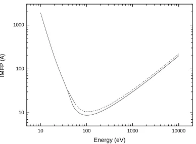
the collective excitations of the electron sea, known as plasmons. Such en-ergy loss mechanisms can be described by calculating the so-called enen-ergy loss function, i.e., the reciprocal of the imaginary part of the dielectric func-tion. The Ritchie theory [17, 20] can be used – starting from the knowledge of the dependence of the dielectric function upon both the energy loss and the momentum transfer – to calculate the differential inverse electron inelastic mean free path and the electron inelastic mean free path. When the elec-tron energy is higher than 50 eV, both the elecelec-tron inelastic mean free path and the electron stopping power calculated within the dielectric formalism are in very good agreement with the experiment (and with theoretical data obtained by other investigators).

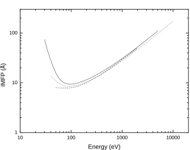
When, on the other hand, the electron energy becomes lower than 50 eV, the dielectric formalism alone is no longer able to accurately describe the en-ergy loss phenomena. In fact, as the electron enen-ergy decreases, the electron inelastic mean free path calculated using only the electron-electron interac-tion increases indefinitely (see Figs. 4.10 and 4.11), while the stopping power goes quickly to zero (see Figs. 4.8 and 4.9). This means that if only electron-electron interactions were active for inelastic scattering, electron-electrons with such a low energy would no longer interact inelastically (i.e., losing energy) with the solid. As a consequence they would travel without any change in their kinetic energy. For a semi-infinite target, this very long travel in the solid would continue forever or until the electron reaches the surface of the material and is able to emerge.

When the energy becomes lower than 20-30 eV, actually, we know that further mechanisms of energy loss becomes very important (electron-phonon and electron-polaron interactions) so that the actual inelastic mean free path approaches zero as the electron energy goes to zero (see Figs. 4.12, 4.13).

4.5

Concluding remarks about scattering

(57)

4.5. CONCLUDING REMARKS ABOUT SCATTERING 57

1 0 1 0 0 1 0 0 0 1 0 0 0 0

1 0 1 0 0 1 0 0 0

IM

F

P

(

Å

)

E n e r g y ( e V )

(58)

1 0 1 0 0 1 0 0 0 1 0 0 0 0

1

1 0 1 0 0

IM

F

P

(

Å

)

E n e r g y ( e V )

Figure 4.11: Present calculation of the inelastic mean free path of electrons in SiO2 due to electron-electron interaction. Solid line represents the present

(59)

4.5. CONCLUDING REMARKS ABOUT SCATTERING 59

0 5 0 1 0 0 1 5 0 2 0 0

1 0 1 0 0 1 0 0 0

IM

F

P

(

Å

)

E n e r g y ( e V )

Figure 4.12: Inelastic mean free path (IMFP) of electrons in PMMA corre-sponding to the various mechanisms of energy loss. Electron-electron inelas-tic mean free path, λinel, is represented by the solid line. Electron-phonon

inelastic mean free path, λp