Socially aware motion planning of assistive robots in crowded environments

(1)

PhD Dissertation

International Doctorate School in Information and Communication Technologies

DISI - University of Trento

Socially aware motion planning of assistive

robots in crowded environments

Alessio Colombo

Advisor:

Prof. Luigi Palopoli

Universit`a degli Studi di Trento

(2)

(3)

Abstract

People with impaired physical or mental ability often find it challenging to negotiate crowded or unfamiliar environments, leading to a vicious cycle of deteriorating mobility and sociability. In particular, crowded environments pose a challenge to the comfort and safety of those people. To address this issue we present a novel two-level motion planning framework to be embedded efficiently in portable devices.

At the top level, the long term planner deals with crowded areas, permanent or tem-porary anomalies in the environment (e.g., road blocks, wet floors), and hard and soft constraints (e.g., “keep a toilet within reach of 10 meters during the journey”, “always avoid stairs”). A priority tailored on the user’s needs can also be assigned to the con-straints.

At the bottom level, the short term planner anticipates undesirable circumstances in real time, by verifying simulation traces of local crowd dynamics against temporal logical formulae. The model takes into account the objectives of the user, preexisting knowledge of the environment and real time sensor data. The algorithm is thus able to suggest a course of action to achieve the user’s changing goals, while minimising the probability of problems for the user and other people in the environment.

An accurate model of human behaviour is crucial when planning motion of a robotic platform in human environments. The Social Force Model (SFM) is such a model, hav-ing parameters that control both deterministic and stochastic elements. The short term plannerembeds the SFM in a control loop that determines higher level objectives and re-acts to environmental changes. Low level predictive modelling is provided by the SFM fed by sensors; high level logic is provided by statistical model checking. To parametrise and improve the short term planner, we have conducted experiments to consider typical human interactions in crowded environments. We have identified a number of behavioural patterns which may be explicitly incorporated in the SFM to enhance its predictive power. To validate our hierarchical motion planner we have run simulations and experiments with elderly people within the context of the DALi European project. The performance of our implementation demonstrates that our technology can be successfully embedded in a portable device or robot.

(4)

(5)

Acknowledgements

First of all, I would like to express my gratitude to my advisor, Prof. Dr. Luigi Palopoli, for his patience, guidance and encouragement throughout the whole Ph.D. ex-perience. His fundamental support helped me to grow as a research scientist.

My sincere thanks to Dr. Daniele Fontanelli and Dr. Sean Sedwards for their support and the several interesting and fruitful discussions we had; and to Prof. Dr. Axel Legay for inviting me as a visiting student at INRIA, Rennes.

Many thanks also to all the people I met within the DALi European project, it was a really great experience.

Finally, I would like to thank my girlfriend Bel´en for her priceless support, I could not have done it without you; my family, to whom this dissertation is dedicated, for their encouragement and patience; and my friends for their endless support and colleagues who I have met in these years.

Alessio Colombo

The research leading to these results has received funding from the European Union’s Seventh Framework Programme (FP7/2007-2013) under grant agreement n◦

ICT-2011-288917 “DALi - Devices for Assisted Living”.

(6)

(7)

List of Tables

4.1 Performance of the long term planner on a BeagleBoard xM . . . 38 5.1 Performance of Scenario 1 . . . 49 5.2 Performance of Scenario 2 . . . 50

6.1 Critical instances interpreted in terms of the taxonomy of behaviours . . . 60 6.2 Identified behavioural rules . . . 61

(12)

(13)

List of Figures

1.1 High level representation of the motion planner . . . 3

1.2 The c-Walker proposed by the DALi project . . . 4

2.1 Diagrammatic overview of the motion planning framework . . . 8

2.2 Overview of the long term planner . . . 10

3.1 Assistive walkers developed in other projects . . . 14

4.1 Diagrammatic overview of the long term planner . . . 20

4.2 Structure of the API . . . 29

4.3 Screenshot of the map designer tool . . . 30

4.4 Graph and a sample path generated from the map shown in Figure 4.3 . . 30

4.5 Simulation with constraints . . . 31

4.6 Simulation with heat map . . . 32

4.7 Simulation with anomalies . . . 33

4.8 Simulation with multiple features . . . 33

4.9 The effect of intensityon Euclidean distance from a desirable zone . . . 35

4.10 The effect of intensityon Euclidean distance from an undesirable zone . . . 36

4.11 Relation between level of crowdedness and effective length of the path . . . 37

5.1 Diagrammatic overview of the short term planner . . . 40

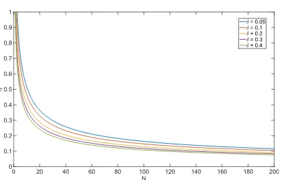
5.2 Relation between number of simulations and statistical confidence . . . 43

5.3 Scenarios used to test the algorithm . . . 48

5.4 Distances of the agents in Scenario 2 . . . 51

6.1 Proxemics zones of the body territory . . . 57

6.2 Experimental set-up . . . 58

6.3 Distribution of behaviours . . . 61

6.4 Instantaneous output of experiment . . . 64

6.5 Trajectories corresponding to experiment shown in Figure 6.4 . . . 65

6.6 Performance of parametrised SFM . . . 65

(14)

7.3 Diagram of the Kalman filter . . . 70

7.4 Unfiltered position compared to Kalman filtered position . . . 73

7.5 Unfiltered speed compared to Kalman filtered speed . . . 74

7.6 The simulated shopping mall created for the DALi experiments . . . 75

7.7 Various pictures from the experimental campaign . . . 76

7.8 Scenario 1 for testing the short term planner . . . 78

(15)

Chapter 1

Introduction

With unimpaired ability, pedestrians are able to find their way across complex and crowded areas without major problems. With reduced abilities this apparently simple task easily becomes a challenging one [1]. For instance, a person with reduced mobility needs to minimise the travelled distance, while a person with cognitive problems should avoid situations that challenge her sense of direction and confuse her perception of the environment. The difficulty in identifying the most correct path and in making proper re-actions to unexpected contingencies may gradually reduce the confidence of the impaired person in using public spaces [2]. The afflicted are most often older adults and the prob-lem worsens quickly if no adequate countermeasure is taken [3, 4]. She can be deprived of essential social relations with a negative impact on her physical condition (reduced exercise), on her psychological wellbeing (reduced social contact) and even on the quality of her nutrition if she reduces the frequency of her visits to supermarkets [5, 6].

A growing body of research [7] suggests that physical activity can have widespread, beneficial effects for older adults and ultimately even decelerate the process of ageing. The application of assistive robotic technologies [8] can be of significant help to amplify these effects. In particular, the type of support that a robotic system with cognitive abilities can offer in the navigation of a complex environment depends on the type of robot assistant and can be adapted to the user’s needs. If the robot is simply a guiding vehicle, like a tour-guiding vehicle [9], guidance just consists in following the path and ensuring that the user is trailing behind. If the robot is a robotic walker, it can guide the user by mechanically turning its wheels and acting on the wheel brakes [10] or by providing visual, audio or tactile signals [11, 12]. If the robot is a robotised wheelchair, it can be compared to a robotic vehicle driving in crowded spaces [13].

(16)

of cleaning the house while the householder is absent, to industrial robots able to move goods in warehouses without human intervention. This trend is visible also in the assistive robotic field and the ability of a robotic platform to navigate crowded spaces in a socially-acceptable manner is becoming increasingly important [14].

Indeed, robots need to understand what is happening around them, so they can choose a course of actions that respects the social rules that govern the environment in which they are moving.

Social rules [15, 16] are non-written rules that manage the cohabitation of people in their environments. If a person is walking and a group of talking bystanders is obstructing her way, she should not pass through them if there are other possible ways around.

If we imagine to substitute this person with a robot, we obtain a human-robot inter-action problem. A robot respecting the social rules will recognise the bystanders, will realise that they are chatting and will identify them as a single cluster that should not be disturbed. Thus, it will modify its planned path to avoid the people without getting too close. However, a robot ignoring these social rules will see the people as two independent obstacles. Hence, it may decide to pass in between them with the consequence of invading their personal space and interrupting the conversation.

Important guidelines for implementing social rules in a robot can be extracted from literature on human social interaction. One example is the work by Goffman [17] that describes the interplay between two people as “focused” or “unfocused” interaction. A focused interaction occurs when one person deliberately searches for the other person’s attention and she responds. An unfocused interaction, instead, takes place when one person finds out information about the other without requiring her attention (e.g., by looking at her behaviour). One interesting theory is proxemic theory by Hall [18] (more details in Section 6.3) that describes the use of personal space and territory, and the relationship between human psychology and non-verbal or iconic communication.

The goal of this dissertation is the design and development of a so called “cognitive engine” for assistive robotic platforms that obeys social rules. Such engine is a motion planning framework that safely steers and controls robots in semi-structured environ-ments populated by human beings while taking into consideration the user’s goals and preferences. We introduce it in Section 1.1.

1.1

Cognitive Engine

(17)

The c-Walker 3

Figure 1.1: High level representation of the motion planner. Initially a coarse long term plan is built on the map by the long term planner. Then, the short term planner is in charge of modifying the short term path in order to avoid obstacles in the surroundings of the platform.

periodically samples the surrounding environment using the sensing capabilities provided by the robotic platform and by the sensors deployed in the environment.

We propose a two-level hierarchical approach, visible in Figure 1.1. A long term plan is first constructed by the long term planner considering both the floor plan and the information gathered from sensors deployed in the environment. During the journey, the short term planner adjusts this path and produces a short term plan that avoids dynamic obstacles detected by the sensors. User preferences and goals are taken into consideration during the whole process.

Further details are reported in Chapter 2.

1.2

The

c-Walker

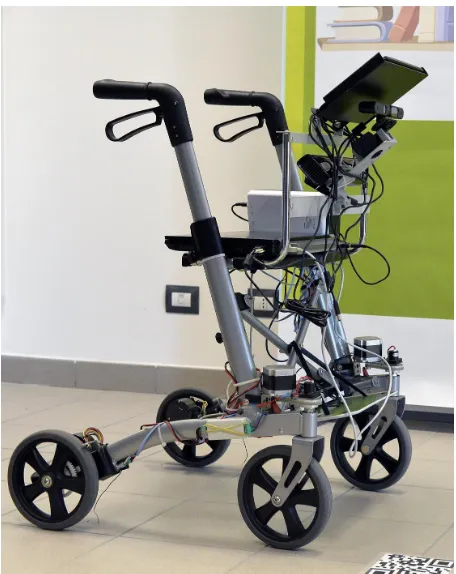
The c-Walker, visible in Figure 1.2, is a kinematically passive haptic device based on a standard mobile robotic platform. Provides physical, cognitive, and emotional support to older adults in public environments such as shopping centres and airports. The user remains always in charge of final decisions and the system does not override her intent. Instead, it operates supportively, offering appropriate recommendations.

(18)

Figure 1.2: The c-Walker is a novel cognitive walking assistant developed within the DALi project. It safely guides the user through complex indoor environments.

the device and the prediction of their future position; 4. the possibility to locally re-shape the path to avoid potential risks and collisions with other humans; 5. a rich set of interfaces that the system can use to recommend a path to the user, which include passive interfaces (visual, acoustic, and haptic) and active interfaces (electromechanical brakes, and motorised turning wheels). These complex functionalities are implemented relying in part on the embedded sensing and intelligence, in part on the ambient intelligence.

The c-Walker prototype has been fully integrated and tested in both synthetic and real environments.

This walker has been developed within the DALi1 _{(Devices for Assisted Living)}

Euro-pean project that targeted a user group consisting of older adults with emerging non-severe cognitive disabilities. Final users have been involved in all phases of the development of the system and the project was acutely sensitive to their needs.

The DALi project ended in October 2014. The ACANTO2 _{(A CyberphysicAl social}

NeTwOrk using robot friends) H2020 European project started in February 2015, and is the follow-up of the DALi project. It will extend the assistive paradigm moving from a

1

http://www.ict-dali.eu/

2

(19)

Scientific Contributions 5

single user to a network of users, connected via a cyber-physical social network.

1.3

Scientific Contributions

This work proposes a hierarchical motion planning algorithm for assistive robotic plat-forms. An overview of this approach has been presented in [19]. The algorithm is able to cope efficiently with dynamic and partially unknown environments, while remaining reactive to potentially uncooperative behaviour of the user.

Three main contributions can be devised:

• Long term planner: an efficient long term motion planner [20] based on the Dijkstra shortest path algorithm [21]. The construction of the path can be customised with soft and hard constraints with priority, and is reactive to temporal anomalies and crowded areas represented as heat maps.

• Short term planner: a probabilistic and efficient short term motion planning algo-rithm for highly dynamical crowded environments [22]. User’s preferences and goals are defined via Bounded Linear Temporal Logic (BLTL) formulae, and enforced using statistical model checking.

• Identification of human motion models: evaluation of a well-known human motion model through experiments with people in a simulated supermarket [23]. Analysis of its limitations and proposal of an extended model.

1.4

Outline of the Dissertation

(20)

(21)

Chapter 2

Overview of the Approach

In this chapter we will give an overview of the proposed cognitive engine. Figure 2.1 shows the logical blocks that compose the motion planning algorithm.

From a top-down perspective, the first type of assistance is offered before starting the navigation activity and consists of the production of a plan that takes into account long term objectives. This is accomplished by thelong term planner (Section 2.1), which takes into account the topology of the space, the user’s preferences and the possible presence of obstacles or problems along the way, which are revealed by environmental sensors. While the user is moving, she could encounter contingent problems that cannot be anticipated (e.g., a small group of people obstructing the path). In this case, her robot assistant could react by planning a minimal deviation from the path that preserves her safety and wellbeing. In our terminology, this component is called theshort term planner (see Figure 2.1) and is introduced in Section 2.2. Finally, the guidance system of the robot assistant can guide the user along the planned path.

In our vision, the user is not required to strictly follow the path, and potential conflicts are detected and resolved automatically without any loss of comfort/safety for the user. During the journey, the motion planner refines its strategy in order to be compliant with the decisions of the user, while reducing the number of conflicts. Every user is associated with a profile that describes specific known interests and dislikes that help the motion planner in generating the path. This profile can be explicitly programmed (e.g., by answering some high level questions) by the user or the caregiver.

2.1

Long Term Planner

(22)

Figure 2.1: Diagrammatic overview of the motion planning framework. The whole process can be divided into three main elements: the long term planner that considers the long term objectives, the short term planner that optimises the long term plan taking into account the short term objectives and constraints, and the guidance that drives the robot towards the goal.

for motion planning, able to identify the path with minimum length (or requiring minimum time) given the a priori knowledge of the map. A first problem is that while the position of most fixed objects (e.g., buildings, rooms, and points of interest) is known a priori, the algorithm must take account of the possibility of changes, such as temporary obstructions. Standard motion planning algorithms can easily be adapted to consider an up-to-date picture of the state of the environment (e.g., presence of obstructions or over-crowded spaces) as it arrives from environmental sensors. However, a simple modification to a standard planner could be insufficient. First, the detected anomaly could be a temporary one. So, the likelihood of having to deal with the problem during the navigation depends on the time needed to reach the place where the anomaly is located, which in turn depends on the chosen path. What is more, the user (who is typically an older adult) will likely have specific additional requirements. For instance, the user could need a frequent access to the toilet, and if the optimum path offers no easy access to the toilet on the way, it could easily generate discomfort. Whereas, the user could be hyper-vigilant and overly concerned with her personal security. In this case, she might appreciate always being within reach of a policeman or of other staff member that she perceives as a reassuring presence.

(23)

Short Term Planner 9

environmental information about the space, such as the availability of services (is the shop that the user wants to visit actually open?), the presence of occlusions and overcrowded areas, etc., 3. preferences of the user (e.g., the need to be in easy reach of assistance, toilets, etc.).

The presence of these specific requirements makes the planning algorithms offered by commonplace navigators (such as Google Maps) infeasible. A different approach that carefully considers the strong psychological aspects involved in the selection of a route is needed.

Thelong term planner periodically collects information from environment sensors and from other c-Walkers deployed on the ground. This information consists of anomalies, heat maps (i.e., crowded areas), status of points of interest (e.g., queue length for shops) and is merged with prior information on the place (the map). The user checks in a request with a sequence of places to visit, and a profile condensing her preferences is attached to it. The long term planner receives the request and produces the optimal path operating as follows: 1. the map is broken down into a grid of discrete cells, 2. a graph is derived from the grid, where each node represents the centre of a cell and each arc is a path joining two cells, 3. the graph is changed by adding relevant semantic information (e.g., associating points of interest with some of the cells), 4. each arc is associated with a cost that accounts for the distance to travel and for the occupancy of the area (people density translates into a longer time to travel), 5. additional manipulations are made to exclude (or to increase the travelling cost of) paths that violate the user preferences, 6. the optimal path is found using the modified Dijkstra algorithm. Figure 2.2 graphically describes this process.

The long term plan is propagated to the system for its execution along with additional constraints related to the user profile that could not be enforced at the level of thelong term planner (e.g., if the user requires not to be in close contact with any other person, this cannot be enforce before the situation in her proximity is known to the system). Then the execution of the desired motion begins and theshort term planner takes over.

Details of the long term planner are extensively presented in Chapter 4.

2.2

Short Term Planner

(24)

Figure 2.2: Overview of thelong term planner. It first takes in input the map of the environment and computes the graph that maps the empty space (top left). The optimal yellow-coloured trajectory connecting start S to goal G can have different shapes according to the objectives: finding the Euclidean shortest path (top right), being closer to the toilets (bottom left), or being reactive to unpredictable anomalies, such as crowded areas or wet floors, (bottom right).

the dynamism of crowd.

The model includes stochasticity to take into account the natural unpredictability of human behaviour, which is exploited by the algorithm to generate multiple independent simulation traces.

Changing the number of simulations can significantly affect performance. The number of simulations can be used as a tuning knob for balancing execution time and statistical confidence. For example, the latter could be temporarily boosted, thus increasing the number of simulations and the time required to compute them, when the system is off-load.

Each of the simulation traces is then formally verified (model-checked) against prop-erties that express goals and constraints required for the user trajectory (i.e., where the user wants to go, minimum distance from obstacles or people). This leads to a statistical distribution of potentially successful trajectories. The algorithm uses this distribution to choose an immediate action that maximises the probability of achieving the objectives of the user while minimising the probability of accidents.

(25)

Identification of Human Motion 11

More details can be found in Chapter 5.

2.3

Identification of Human Motion

The ability to understand human behaviour and social interactions is of primary impor-tance. The goal is to identify an accurate two dimensional model for predicting human motion. Our starting point was the Social Force Model (Section 6.2), generally used for simulating people in normal or panic situations. This model is very flexible and broadly used in the literature. However, in some cases it does not produce realistic motions, es-pecially when the trajectories of pedestrians are interrupted by sudden short term pauses and deviations.

We thus started by observing people in a real scenario, running controlled experiments in a simulated supermarket, where several people concurrently had to follow their shop-ping list. The videos of the experiments were then manually labeled according to the observed behaviours, and we were able to match the observation with proxemic theory. Proxemics (Section 6.3) is an important theory borrowed from the literature on human social interaction, and relates human psychology with spatial behaviour.

These results helped us to identify a number of behavioural patterns that can be incorporated in an extended version of the Social Force Model.

(26)

(27)

Chapter 3

Related work

The purpose of this chapter is to relate the work presented in this dissertation with the current state of the art. We start with an overview of similar projects for assistive robotics in Section 3.1, then a survey of the literature for the different components that compose the motion planner.

Motion planning in crowded environment is a relevant research problem in robotics that has received a constant attention throughout the past two decades [24, 25, 26]. The approach that we advocate is based on a hierarchical decomposition of the problem between short term and long term planning. Different authors in the literature propose a strategy of this kind [27, 28], but the solution at each of the two levels of the hierarchy differ significantly based on the requirements that each author considers.

Thelong term planner is discussed in Section 3.2, theshort term planner in Section 3.3 and the identification of human motion models in Section 3.4.

3.1

Assistive Robotics

Several projects have targeted assistive mobility with the development of a robotic walking assistant and some of them share the basis ideas with the DALi project.

The ASSAM project [29] aims to develop a modular navigation assistants for users with different level of disabilities. They target different mobility platforms, such as tricycle, wheelchair and walker. The latter is called eWalker (Figure 3.1(a)) and is an electronic walker providing navigation support by means of an active platform that compensates declining walking capabilities, as well as cognitive disabilities. However, the behaviour of people in the surroundings is not considered.

(28)

(a) ASSAM [29] (b) DOMEO [30] (c) I-DONT-FALL [31] (d) Veloped [32]

Figure 3.1: Assistive walkers developed in other projects.

the proposers’ point of view, the older adults should be helped in staying longer and safer at home. This is clearly in contrast with the DALi project that actually encourages the elderly to socialize and move in large public spaces.

The i-Walker, showed in Figure 3.1(c), is the assistive device developed within the I-DONT-FALL project [31]. The main goal of the project is to improve quality of life of the elderly through the efficient prevention and detection of falls. The device is part of an ecosystem of healthcare services and is used for physical training and data logging.

The Veloped [32] (Figure 3.1(d)) is a commercial walking support for outdoor explo-ration with an appealing look. Different versions are available according to the target outdoor environment. Some of them are passive and exploit only the mechanical design for easing the walk. Others, instead, are equipped with motorised wheels for providing aid on critical terrains.

3.2

Long Term Planner

(29)

Long Term Planner 15

path can be found by exploring the data structure. The more time that is given to the computation, the more points that can be added and the higher the probability becomes of finding an optimal solution. Such algorithms have recently been revisited by Karaman and Frazzoli [35]. The revised versions, PRM∗ _{and RRT}∗_{, are probabilistically complete,}

meaning that if the algorithm is given enough time to explore the space, it eventually identifies the optimal solution with probability 1. An important point of these algorithms is that while the data structure is being created it is possible to enforce a hierarchy of hard and soft constraints penalising (or ruling out) points that would violate them. This is an appealing feature for us because our problem is characterised by a set of constraints. However, the construction on the fly of the path and on the map is not required in our case. Our intended operational scenario is a public space (e.g., a mall or a museum) for which a large amount of a priori information is usually available.

Another family of algorithms are based on the definition of potential fields [36, 37] around obstacles and points of interest that can attract or repel the robot. Such ap-proaches are known to be effective for obstacle avoidance, but they are often plagued by local minima (which sometimes delay or deadlock the progress). While encoding all the user’s planning requirements, constraints and preferences with a potential function is generally a difficult problem, our approach makes use of the notion of gradients to encode user-defined desirable and undesirable zones. The full details are given in Section 4.2.3

The long term planner proposed in this work falls in the class of graph based tech-niques. In essence, the idea is to decompose the environment into a grid and then generate a graph by associating nodes to elements of the grid and by then connecting with arcs the nodes associated to adjacent cells. Minimum time paths on the graph can be found using the well-known Dijkstra algorithm [21] or its extension A∗ _{[38]. The use of a constant}

size grid is generally discouraged due to the explosion of the configuration space size, hence several more efficient ways to construct the graph have been proposed. Possible approaches include Voronoi diagrams [39] and PRM [33]. We follow Chen et al. [40] and construct a graph using quad tree decomposition of the space, exploring it with an ex-tended version of the Dijkstra algorithm. The generation of our quad tree is specific for its application to structured indoor spaces, with large rooms connected through corridors, doors and passageways and where each room may contain such things as counters, shelves and exhibition paraphernalia that compromise its regularity.

(30)

itself as a clear winner. In our particular case, we adopt a conservative assumption, described in Section 4.2.6, that allows us to solve a simplified problem very efficiently. Our requirement analysis reveals that senior users of a navigation tool are very annoyed by a long wait in front of a screen. Therefore, efficiency and quick deliveries of decisions are more important than producing “optimal” decisions (as long as the decisions do not violate any hard constraints and they respect soft constraints to a reasonable extent).

The global constraints (not to be confused with kinodynamic constraints, not consid-ered here) are used for customising the behaviour of the planner and for introducing the notion of “comfort” for the user. Constraints are prioritised and some of them can be violated if their compliance prevents the system from finding any path.

They embed priority and the possibility for one or more constraints to being ignored if a path cannot be found otherwise (namely, conflicting constraints). This is called “planning with partial satisfaction”, and is studied in the literature under the notion of preference-based planning. In [45] they focus on computation of relaxed plan-based heuristics that guide the planner towards good solutions satisfying the given preferences. In [46] they introduce a method for quantifying the satisfaction of linear temporal logic (LTL) formulae, and propose a planning framework using this method to synthesise robot trajectories with the optimal satisfaction value. However, they do not consider constraints where the cost or priority changes over time. Tumova et al. [47] present an automatic generator for control strategies for a robotic vehicle where constraints are expressed with LTL formulae. The novelty is the possibility of violating a constraint, according to its priority, in order to complete the task (e.g., a road lane should not be crossed, but this is allowed during car parking).

The concept of “comfort” has already appeared in the literature but generally with different meanings: 1) comfort of the user when navigating using a robotic platform [48, 49] and 2) comfort of the humans in the area surrounding an autonomous robot [50]. Our notion of comfort belongs to the first class and it is deeply rooted in the requirement analysis and in the validation activities with senior users that we have been conducting in the context of the DALi and of the ACANTO projects. Our findings are that the user needs to specify zones that she likes or dislikes. As an example, more often than not she would prefer to bypass crowded areas or to always have a toilet or a resting place within easy reach, even if this entails choosing a slightly longer path.

3.3

Short Term Planner

(31)

Identification of Human Models 17

that predict behaviour based on models parametrised with data from sensors (e.g., [55]). In common with existing sampling methods, our algorithm uses randomisation to cover an intractably large configuration space. In contrast to many existing uses of sampling, however, we do not assume a fixed environment. In our application the environment contains both fixed and dynamic elements, such that a single optimal path cannot be defined a priori. Hence, the problem we solve by sampling is not one of creating an optimal long term plan, but one of finding an optimal short term plan given a changing environment.

Model checking is an automatic process to verify that a system satisfies a property specified in temporal logic. In the present context, temporal logic can express complex dynamical properties such as “the user will visit all the desired locations in a specified sequence, within the specified time” and “the user will never get too close to any other pedestrian”. If the notion of an optimal path can be so defined, the principles of model checking can be used to directly synthesise a ‘correct’ motion planner or to prove that an existing motion planner is correct [52, 53, 54]. The use of probabilistic model checking in combination with the theory of stochastic hybrid automata [56] is particularly appealing for control and robotic applications where a non-zero probability of failing the mission can be tolerated. For example, in [57, 58] for air traffic control or in [59, 60] for industrial robotics. Combining model checking with sampling, algorithms can be constructed which provably converge to optimal schedulers [54]. Standard model checking algorithms are computationally intensive, hence existing applications have used model checking offline. By using statistical model checking, we are able to perform online verification. We do not prove correctness, but we find a short term plan that maximises the probability of success.

3.4

Identification of Human Models

Basically two main approaches exist in the literature for modelling human motion. The first one proposes a single model that captures the features of the human motion. The second one relies on different dynamic models that are combined using a switching logic. One advantage of the first approach is that it is easier from a computational point of view, while with the second one it is easier to highlight the different decision points that compose the human behaviour.

(32)

and models them as attractive (e.g., friends, points of interest), and repulsive forces (e.g., walls, strangers). Its strengths and weaknesses are well tested and understood [62, 63, 64]. However, the resulting behaviours strictly depend on the input parameters, which are not easy to estimate.

L¨ammel et al. [65] presented an interesting comparison between some models for pedes-trian dynamics and the real world. Specifically, they investigated three approaches (in-cluding the SFM) and their ability to reproduce collision-free movements in dynamic environments.

Kelly et al. [66] proposed a switching model that combines constant acceleration, constant velocity and constant position models with a Kalman filter. The switching logic is based on the statistical properties of the innovation sequences computed by the filter.

Moussa¨ıd et al. [67, 68] focused on social groups and how the self-organisation mech-anism of people affects crowd dynamics.

Burstedde et al. [69] proposed to track pedestrian dynamics using a two-dimensional cellular automaton.

Lau et al. [70] proposed a multi-model for group tracking and group size estimation. They have a set of hypotheses (e.g., split, merge and continuation) that they validate on the observed data. However, in their case the microscopic motion of a single person loses importance, in favour of the behaviour of the whole group.

(33)

Chapter 4

Long Term Planner

This chapter goes into details of thelong term planner. The algorithm and its validation are presented in the following sections, where both qualitative and quantitative results are given.

4.1

Preliminaries

The proposedlong term planner has been developed bearing in mind a number of require-ments. The key point is letting the user personalise her journey while keeping the planner reactive to changes in the environment. For this reason we have implemented three main features.

The first feature gives the user the possibility of adding hard (non-violable) and soft (violable) constraints, according to some customisable priority. It is possible to encode rules like “never get closer than 5 meters to any stair” or “try to keep within 10 meters of a toilet”, or “always be within sight of a clerk or of a policeman”. Should a soft constraint be in conflict with another one, the issue is resolved by violating the one with lower priority. A hard constraint, instead, cannot be violated.

The second feature reacts to anomalies detected in the environment by the sensing subsystem. An anomaly is a bounded zone in the environment that becomes inaccessible for a limited period of time (e.g., a wet floor or blocked passage). After this period expires, the anomaly is cleared and the zone is accessible again.

The last feature takes into account the crowded spots in the environment. They are represented as heat maps (an example is shown in Figure 4.6) where the apparent “heat”

Part of this chapter was published in

(34)

Figure 4.1: Diagrammatic overview of the long term planner. Informed by the heat maps and anomaly detectors, the long term planner constructs a long term plan according to the user’s constraints. The plan is then transferred to the control subsystem.

represents the level of crowdedness. The planner interprets this level as a penalising factor that slows down the user. Some users could also have specific constraints related to avoiding crowded areas.

The work flow of the algorithm begins with the user specifying a list of target locations she wants to visit in the environment. The long term planner constructs a plausible path (a long term plan) according to the constraints in the user’s profile and to the current conditions in the environment (known anomalies and current crowding represented by heat maps). This data is sampled periodically from remote sensors (e.g., surveillance cameras). If other robots are deployed in the environment, they can use their local sensing system to detect anomalies and share this information through a cloud infrastructure. For instance, if a walker detects a wet floor sign, this information is propagated to the other robots and accounted for in the generation of long term plans. Once the user accepts the plan and starts moving, the control subsystem takes over, allowing the short term planner to make limited adjustments depending on the contingencies encountered on the ground. In the event that the user is unable to follow the plan with only such limited modification (e.g., an unforeseen obstacle), the control subsystem has the capability to report the event and can request the construction of a new long term plan.

(35)

Planning Algorithm 21

changed by adding relevant semantic information (e.g., associating points of interest with some of the cells), 4. each arc is associated with a cost that accounts for the distance to travel and for the occupancy of the area (the more people, the longer the time to travel), 5. additional manipulation are made to exclude (or to have a negative reward for) paths that violate the user preferences, 6. the optimal path is found using the modified Dijkstra algorithm.

In the next sections the algorithm is presented in its full details.

4.1.1 Preliminaries

To describe our long term planner, we first define some notation and operations on graphs. A graph G= (N, E) is a set of nodesn ∈N linked by a set of edges e∈ E. An edge

e= (n, n′₎_∈_E _{is defined by its two adjacent nodes} _{n, n}′ _∈_N_.

Given graphs G1 = (N1, E1) and G2 = (N2, E2), G1 ⊆ G2 =⇒ N1 ⊆ N2∧E1 ⊆ E2

means thatG1 is a subgraph of G2.

Given G1 ⊆ G2, G2\G1 = (N2\N1, E2\{e ∈ E1 |e = (n, n′)∧(n ∈ N1∨n′ ∈ N1)} is

the graph that remains after removingG1 fromG2. We do not considerG2\G1 ifG1 6⊆G2

Pairwise graph union is defined byG1∪G2 = (N1∪N2, E1∪E2). The union of a set of

graphsG ={G1, G2, G3, G4, . . . , Gm} is denoted SG and performed pairwise, such that

S

G=((· · ·(((G1∪G2)∪G3)∪G4)∪ · · ·)∪Gm).

4.2

Planning Algorithm

The long term planner proposes feasible paths that efficiently visit the user’s specified points of interest, while respecting the user’s preferences and accommodating the pre-vailing conditions in the environment. To achieve this, the long term planner abstracts a complex environment, such as a shopping mall, airport, museum, etc., as a weighted directed graph, comprising a set of nodes linked by edges. The nodes represent places in the environment, while the edges represent direct paths between the places and are weighted by theireffective length. The a priori length of an edge is the Euclidean distance between its adjacent nodes. The effective length of an edge is generally longer, modelling its undesirability with respect to crowding and the user’s preferences.

(36)

by simply modifying the graph prior to finding the shortest path. In particular, anoma-lies cause parts of the graph to be (temporarily) removed, while crowding increases the weights of edges in crowded areas (their effective length is increased because crowding slows the user’s progress). Certain user preferences, such as always being near a toilet, may also be encoded as graph transformations.

4.2.1 Creating graphs from floor plans

To construct a graph that efficiently maps the free space in the environment, we first decompose its floor plan into a ‘quad tree’ [72], comprising quadrants containing free space (free quadrants) and quadrants occupied by fixed objects (occupied quadrants). A graph is constructed by embedding nodes in only the free quadrants and linking them with appropriate edges. The quad trees typically have substantially fewer cells than a uniform grid with the same level of minimum granularity, with the density of cells generally following the density of features [73]. An example is shown in Figure 4.4.

Given a quad tree decomposition of the free space, the corresponding graph is con-structed as follows. For all pairs of adjacent free quadrants, a node is embedded at the mid point of the border of the smaller of the quadrants. By definition, a free quadrant is a convex shape containing only free space. Hence, any node on the border of a free quadrant has a “line of sight” to all other nodes on the borders of the same quadrant. We therefore join such nodes with a complete graph. Since nodes are shared between adjacent quadrants, this is sufficient to link all the free space in the environment.

To guarantee that the robotic platform may occupy any point in free space represented by a node, or travel the line represented by any edge, prior to building the quad tree the fixed objects are enlarged in all directions by a distance greater than the radius of the robotic platform. In this way no point in the effective free space is ever too close to a fixed object and all paths in the graph correspond to plausible paths in the environment.

4.2.2 Creating a long term plan

To represent the a priori knowledge about the environment we define a “graphmap” data structure M= (G, W, C, L). G = (N, E) is a graph of the environment derived from a quad tree, as described in Section 4.2.1. Function W : E → (0,+∞] assigns a length (the Euclidean distance between the points denoted by adjacent nodes) to all the edges of the graph. Function C :N →(Q,Q) labels each node with its spatial coordinates in the environment. Function L : N → P ∪ {uninteresting} labels each node with its semantic location, where P ={supermarket, bakery, caf´e, etc.} is a set of points of interest.

(37)

working graphmap), modified according to the user’s constraints, the current crowding and the known anomalies. We denote the working graphmap M′ _{= (}_G′ _{= (}_N′_{, E}′₎ _⊆

G, W′_{, C, L}_{). In general, the graph} _G′ _{excludes any inaccessible subgraphs arising from}

anomalies or the user’s constraints. The weighting functionW′ _{assigns an}_effective _length

to all edges, which includes the effects of crowding and the user’s constraints. The con-struction of G′ _and _W′ _{are described in Sections 4.2.3, 4.2.4 and 4.2.5.}

Given a working graphmap M′ _{and a (possibly ordered) set of user-specified points}

of interest, the long term planner proposes a path that visits the points of interest while respecting the user’s global constraints. Formally, given a user-specified set of points of in-terest{pj ∈P}jm=1, the planner suggests a path{ni ∈N′}ki=1 s.t. ∀pj ∈ {p1, . . . , pm} ∃ni ∈

{n1, . . . , nk} ∧L(ni) = pj. If the path must respect the order of the specified points of

interest, then additionally ∀ps, pt ∈ {p1, . . . , pm},∄ni, nj ∈ {n1, . . . , nk}s.t. s > t∧i <

j∧L(ni) =ps∧L(nj) =pt holds true.

Finding the minimum length path that visits a set of unordered points of interest is an instance of the well known NP-hard ‘travelling salesman problem’ [74]. Moreover, given that the overall excursion (including stops at the points of interest) may take considerable time, an overall plan optimised for the current level of crowding may eventually be sig-nificantly sub-optimal if the crowds dissipate. Our approach is therefore to optimise each leg of the journey separately, using the most up-to-date information about anomalies and crowding.

In general and in simple terms, long term planning works in the following way. The planner first identifies the node n0 ∈ G′ that is closest to the user’s current coordinates

(x0, y0). This is given by n0 = arg minn∈G′ k C(n)−(x₀, y₀) k. If the user’s points of

interest have been specified in order, the planner uses Dijkstra’s algorithm to find the shortest path betweenn0 and the next unvisited point of interest specified by the user. If

the user has not specified an order, the planner uses a modification of Dijkstra’s algorithm to find the shortest path between n0 and the closest unvisited point of interest. Given

the trajectory and the user’s coordinates, n0 may not be the optimum first node in the

path (it may be effectively behind the user on the path). The planner therefore sets the first node of the path to be the node by which the user will leave the current quadrant.

The inclusion of time-dependent anomalies makes the actual long term planning algo-rithm slightly more complex. Handling such anomalies is described in Section 4.2.5.

4.2.3 Global constraints

(38)

don’t get too close to other pedestrians). Global constraints may be hard or soft. Hard constraints exclude parts of the environment that the user does not wish to visit under any circumstances. They are implemented by removing subgraphs from G. The set of hard constraints is denoted x ∈ X, x ⊆ G, hence G′ ₌ _G_\S

X. Removing parts of the graph may significantly lengthen the planned journey or make it impossible, hence the final plan (or lack of it) is presented to the user for approval.

Soft constraints make parts of the environment desirable or undesirable to the long term planner, causing the planned path to deviate towards or away from them, respec-tively. They are implemented by defining a function K : E → [1,+∞] that modifies the weights of edges to and from desirable and undesirable nodes. The function K is applied according to (4.1), introduced in Section 4.2.4. If no constraint applies to the nodes adjacent to edge e then K(e) = 1. In general, given two nodes n and n′

con-nected by edges e = (n, n′_{) and} _e′ _{= (}_n′_{, n}_{), for a single constraint} _K₍_e₎ _{> K}₍_e′₎ _⇐⇒

n is more desirable than n′_{. In the case of multiple constraints applying to the same edge}

e, the value of K(e) is the maximum considering all constraints.

In our implementation, soft constraints are specified using sets of triples (location, radius,intensity), which respectively define the semantic position, the radius of influence and the intensity of the constraint. In general, a constraint creates a gradient of weights that increase towards undesirable zones and vice versa for desirable zones.

We define a function ˜Ki : [0, radius] → [1, intensity] that maps distance from the border of location i to the weight of the gradient. This function should be monotonic non-increasing in case of undesired locations, and monotonic non-decreasing in case of desired locations. In both cases its integral should be finite (i.e., the radius of influence should be finite). Function ˜Ki is later used by K(e) for associating the weight to each edge. It is worth noting that there is high flexibility in the choice of ˜Ki, which improves the expressiveness of global constraints, allowing per-user customisations (e.g., the profile of attraction to toilets might be different across users) as well as location based person-alisation (e.g., the profile of repulsion of an open window is different from the one of a stair).

More formally, we assume the existence of a set of constraints s ∈ S. The location of each constraint defines a corresponding set of either desirable or undesirable nodes

Ns ⊆N that are not necessarily disjoint. Letd(i, j) denote the minimum Euclidean path distance from node i to node j, then for any edge e = (n, n′₎ _∈ _E_{, the value of} _K₍_e_{) is}

given by

K(e) = max

∀s∈S

K∗

locations

min n′′_∈_Ns

(39)

where K∗

locations is defined as:

Klocation∗ s(r) =



 

 

˜

Klocations(r) if r∈[0, radius]

1 otherwise

4.2.4 Heat maps

Cameras in the environment monitor pedestrian traffic and construct “heat maps” that estimate average occupancy of the free space over useful time periods (e.g., the last five minutes or a long-term average for a particular day and time). Each point in the free space is thus assigned a value in the interval [0,1], denoting its time-averaged occupancy density. A point with average density 1 is effectively impassable. In practice, not all areas are monitored and monitored areas will be divided into an array of square cells of uniform local density. Unmonitored areas are assumed to have zero density. Areas occupied by fixed objects have density 1.

An edge represents a straight line path between the points in free space represented by its adjacent nodes. The average occupancy in the area surrounding the line affects the time taken to travel from one end to the other. The free space that the short term planner will allow the user to explore can be approximated by an ellipse whose vertices (“ends”) coincide with the ends of the line. The area of the ellipse represents the capacity of the edge, while the heat within the ellipse represents the amount of capacity that is being used by others. To calculate the average occupancy of an edge, we integrate the occupancy density over its corresponding ellipse. The size and shape of the ellipse is a function of the edge. For simplicity we define an occupancy functionH :E →[0,1] that implicitly includes knowledge of the current heat map and performs this integration. The effective length of an edge is then given by the function W′ _:_E _→₍₀_,₊_∞_{], defined}

W′(e) = K(e)W(e)

1−H(e) ∀e∈E. (4.1)

The intuition behind (4.1) is that the effective length of an edge e is proportional to the desirability K(e) of the destination node and inversely proportional to the occupancy

(40)

4.2.5 Anomalies

During the course of a journey the user may encounter anomalies (semi-permanent ob-structions, such as a wet floor, locked exit, dense crowd, etc.) that prevent theshort term planner from making progress along the long term plan. An anomaly is represented by a data structure (g ⊂G, t ∈(0,+∞]), where g ⊂G represents the inaccessible region of the environment and t is the estimated remaining time that the anomaly will last. The set of active anomalies (those with remaining time >0) is denoteda ∈A. Anomalies are removed from A when their remaining time reaches 0.

Anomalies exclude parts of the environment, but their effect is not permanent and is dependent on the chosen path. When a new anomaly (g, t) is detected by the short term planner, it is added to the set of active anomalies and its subgraph is immediately removed from the working graphmap. Symbolically, A ← A ∪(g, t) and G′ _← _G′_\_g_.

The shortest path to the next point of interest is calculated according to the procedure described in Section 4.2.2. The approximate time of reaching every node in the proposed path is calculated according to the average speed of the user.

The new trajectory definitely excludes the recently detected anomaly, but may include one or more anomalies inA. Hence, the proposed plan is compared to the subgraphs in the set of active anomalies, to find if there is any intersection. If there is no intersection the proposed plan is valid. If the proposed trajectory intersects the subgraph of an anomaly, the time of reaching the anomaly is compared to its remaining time. If the anomaly will not exist by the time the user reaches it, it is ignored. If no anomalies exist by the time the user reaches them, the proposed plan is valid. If, on the other hand, one or more anomalies remain valid by the time the user reaches them, their subgraphs are removed from the working graphmap and the above procedure is repeated until a valid path is found.

4.2.6 Time-dependent shortest paths

(41)

Implementation Aspects 27

the same point of interest.

Algorithm 1 describes the basis of our shortest path algorithm that considers timed anomalies, heat maps and user constraints. The algorithm finds the shortest path between the user’s current position and the closest point of interest. If points of interest are required to be visited in a specific order, it is assumed that the setTargetscontains only those nodes corresponding to the next point of interest to visit.

The algorithm makes use of several functions. K(e), W(e) and H(e) are as in (4.1). Function Edges(n) returns the set of outgoing edges of node n. Function Dest(e) returns the destination node of edge e. Function Anomalytime(e) returns the absolute time at which edgee will be available. This function returns 0 for all edges that are not part of an anomaly. Two functions are updated during the planning process. Function Dist(n) returns the currently known shortest distance to noden. This is initially∞ for all nodes except the initial node, for which the function returns 0. Function Time(n) returns the estimated time to reach node n given the user’s average speed (denoted speed). The function initially returns ∞ for all nodes except the initial node, for which it returns 0.

In trying to satisfy the conflicting constraints of dynamic motion planning in com-plex human environments, we have considered many alternatives and refinements to our algorithms. There is no off-the-shelf perfect solution, given the inherent uncertainties and variability of the problem. In particular, finding time-dependent shortest paths is known to be hard and is itself the subject of active research [41, 42, 43, 44]. Our present approach is a satisfactory compromise between efficiency and efficacy. We can imag-ine circumstances under which it might be challenged, but we propose to allow further development to be led by problems encountered in real applications.

4.3

Implementation Aspects

The algorithm presented in this work has been designed keeping flexibility in mind. We devised an API that abstracts the low level structures and exposes a simple but efficient interface. It is divided into a number of layers visible in Figure 4.2. The bottom layer is represented by thelong term planner itself, which is linked with the top level (the API) via three main blocks.

(42)

Algorithm 1 Shortest path considering anomalies, heat and constraints The initial node is the closest node to the user

Targets: a set of target nodes corresponding to the user’s points of interest

Visited: a set of visited nodes, initially containing the initial node

Unvisited: a set of unvisited nodes, initially containing all nodes except the initial node

current←initial node

whilecurrent6∈Targetsdo

for all e∈Edges(current) do

if Dest(e)∈Visited then continue

end if

if Anomalytime(e)>Time(current) then continue

end if

d←Dist(current)K(e)W(e)/(1−H(e))

if Dest(e)∈Unvisited then if d >Dist(Dest(e))then

continue else

Unvisited←Unvisited\{Dest(e)}

end if end if

Time(Dist(e))←Time(current) +W(e)/(1−H(e))/speed

Dist(Dest(e))←d

Visited←Visited∪ {Dest(e)}

end for

Visited←Visited∪ {current}

Unvisited←Unvisited\{current}

if |Unvisited|>0then

current←n∈Unvisited:

Dist(n)≤Dist(n′₎_,_∀_n′ _∈_Unvisited

else

report no possible path and quit

(43)

Implementation Aspects 29

Long term planner API

Cloud services Environmental

monitoring

Smartphone APP

Heat maps Anomalies

Environment and map

Constraints User profile Plan

Figure 4.2: Structure of the API. The layers are of increasing abstraction, where the public interface is flexible and extensible at runtime by the third-party services. The overall low complexity enables a broad choice of implementations, from a service in the cloud to a standalone smartphone app.

The second block, “Plan”, exposes the planning capabilities. Given the starting po-sition, it is possible to query for the construction of the optimal path directed to one or more goals. The planner automatically considers the current status of the environment and biases the resulting trajectory according to the user preferences. Moreover, alterna-tive sub-optimal paths can be generated upon request, for example when the chosen path is blocked by an unforeseen obstacle detected by the short term planner.

The last block is the “User profile” and encapsulates the interface for accessing the global constraints and other user information, such as her location and the tuning param-eters for dealing with anomalies and crowded areas.

This API can be installed and accessed practically anywhere, thanks to the low com-putational burden highlighted in Section 4.5.3. For example, it can be packaged in a standalone mobile application for providing the users an interactive map of a shopping mall, or implemented as a cloud service, as described in the next section.

4.3.1 Implementation of a Cloud Service

(44)

Figure 4.3: Screenshot of the map designer tool showing an example floor plan. Enables the user to create maps and generate the associated graph, compliant with the long term planner.

X [m]

0 2 4 6 8 10 12 14 16 18 20

Y [m]

0 1 2 3 4 5 6 7 8 9 10

Goal Start

Figure 4.4: Graph and a sample path generated from the map depicted in Figure 4.3.

these elements.

The map of the environment is stored using SpatiaLite1_{, a lightweight serverless spatial}

database that allows performing queries in the geometric space. A quad tree decomposi-tion is then performed on the map and the resulting graph is used by the planner.

The communication with the remote clients takes place through exchange of JSON messages over a TCP link, in a request-reply mechanism, where the planner acts as a server.

4.4

Qualitative Analysis

We have implemented two tools, a map designer and a simulator. The map designer is written in MATLAB and enables the user to draw, load and save floor plans, as well as

1

(45)

Qualitative Analysis 31

X [m]

0 2 4 6 8 10 12 14 16 18 20

Y [m] 0 1 2 3 4 5 6 7 8 9 10 Goal Undesired Desired Start

Figure 4.5: Simulation with constraints. The picture shows two independent simulations of how the planner deals with desirable and undesirable zones. The continuous line is the result of the constraint “stay close to the desirable zone” and “stay away from the undesirable zone”, while the dashed line addresses only the latter.

performing quad tree decomposition and graph construction. The user is provided with a GUI to freely draw geometric shapes (Figure 4.3) and generate the corresponding graph (Figure 4.4) to be used in the simulator.

The simulator is written in MATLAB and Java and allows the user to visually configure global constraints, heat maps, anomalies and all parameters required by the long term planner. For performance reasons, the planning algorithm has been developed in Java and communicates with MATLAB through the integrated Java interface.

The chosen floor plan for the validation is a large room of approximately 200 m2 _with

two non-aligned central columns. The starting point is set at the left hand side of the map in the midway along the shortest wall. The goal is set at opposite side of the room, such that the shortest path connecting the starting point to the goal is a straight line.

In the remainder of this section we will go through each feature separately and, finally, show a more complex simulation combining different features.

We show how the planner is able to deal with the user preferences when computing the plan. In the first simulation we put an undesirable zone in the middle of the room, overlapping the shortest path. In the second simulation, instead, we identified a desirable zone (e.g., a restroom) close to the top wall of the map without interfering with the shortest path. In both simulations the minimum distance to the zones is set equal to 1.5 m and the intensity is set to 2.

(46)

X [m]

0 2 4 6 8 10 12 14 16 18 20

Y [m]

0 1 2 3 4 5 6 7 8 9 10

Goal Start

Figure 4.6: Simulation with a heat map. The path computed by the planner is represented by the continuous line and bypasses the crowded spot in the middle of the map (i.e., yellow zones). The preference is for cold zones (i.e., blue-coloured areas).

the original shortest path.

Should the undesirable zone be the only possible access point for reaching the goal, the planner can violate the constraints as long as the intensity is not −∞ (i.e., never touch the undesirable zone).

4.4.2 Heat maps

We placed one rectangular shaped heat map in the centre of the room, covering the whole space between the two columns and the walls at the top and bottom of the figure. The planner is thus forced to go through the area covered by the heat map to reach the goal. We ran 50 simulations with different heat distribution generated by a sum of bivariate Normal probability density functions (normalised between [0,1]) with random parameters. In all cases the planner correctly took into account the presence of the heat map.

The outcome of one particular simulation can be seen in Figure 4.6, where the planner properly avoids hot (yellow-coloured) zones.

4.4.3 Anomalies

(47)

Qualitative Analysis 33

X [m]

0 2 4 6 8 10 12 14 16 18 20

Y [m] 0 1 2 3 4 5 6 7 8 9 10 Anomaly Goal Start Anomaly expires

Figure 4.7: Simulation with anomalies: two independent simulations are shown. The dashed line represents the path generated when the anomaly is set to expire half way to the goal. The continuous line, instead, shows the resulting path when the anomaly does not expire.

X [m]

0 2 4 6 8 10 12 14 16 18 20

Y [m] 0 1 2 3 4 5 6 7 8 9 10 Anomaly Start Undesired Desired Goal

Figure 4.8: Simulation with multiple features. The planner satisfies all the user requests, but is forced to ignore the constraint for the undesired zone, as it is the only way for reaching the goal.

user reaches the goal position. It is clearly visible that, in the first case, as soon as the anomaly expires the planner re-routes the user towards the shortest path, overlapping what was the area occupied by the anomaly.

4.4.4 Combination of features

(48)

4.5

Quantitative Analysis

We now go through the results of some simulations providing a quantitative analysis of the performance of the long term planner. The goal is to show that the benefits of using the long term planner are evident not only from a qualitative point of view, as shown in Section 6.4, but also from a tangible set of performance metrics.

The simulations presented in this section show how the planner interprets the intensity parameter of an undesired or a desired global constraint. The environment and the posi-tion of the desired/undesired locaposi-tions are the same as those considered in Secposi-tion 4.4.1 and illustrated in Figure 4.5. We identified this particular scenario because it is a worst case situation: the desirable locationis at the farthest possible distance from the shortest path and the undesirable locationconflicts with the shortest path.

For simplicity and without any loss of generality, in these simulations we define ˜K as a linear function that is monotonically increasing for desired constraints, and monotonically decreasing for the undesired ones.

To measure the characteristics of a constraint for a desirable zone, we set thelocation as far as possible from the Euclidean shortest path and we fixed theradiusto a large value. We then iteratively executed the planner with increasing intensity and we computed the minimum direct Euclidean distance of the path from the location (i.e., not considering the graph). The results are reported in Figure 4.9. As expected, the minimum Euclidean distance between the path and the desirable zone decreases as intensity increases. The steps in the plot are due to the quantisation of the free space imposed by the underlying graph.

(49)

Quantitative Analysis 35

Intensity

0.01 0.1 1

Euclidean distance [m]

0 2 4 6 8 10 12 14 16 18 20

Figure 4.9: The effect ofintensityon the minimum Euclidean distance from a path to a desirable zone on a particular simulation run. As intensity increases the path is attracted towards the desirable location: the Euclidean distance decreases.

4.5.2 Heat maps

We demonstrate that the long term planner is able to provide better (i.e., quicker) tra-jectories when it is aware of the crowdedness in the environment.

We set up a simulation similar to the one in Section 4.4.2, where the heat map covers the environment as in Figure 4.6. We then iteratively increase the heat surface, simulating an expanding crowd, starting from no crowd (0% crowdedness) up to a completely crowded area (100% crowdedness). At each iteration we call thelong term planner and we compute both the optimal path (e.g., considering the heat encoded in the effective distance) and the Euclidean shortest path (e.g., a straight line directed to the goal that passes through the crowded area).

The Euclidean shortest path Ne ={ni ∈ N′}ki=i is constructed by assuming H(e) = 0 in (4.1). The true costWe ofNe is then computed by removing theH(e) = 0 assumption, thus

We =

X

W′₍_e₎_,_∀_e _{= (}_{n, n}′₎_∈_N

e

(50)

Intensity

1.5 1.6 1.7 1.8 1.9 2 2.1 2.2 2.3 2.4 2.5

Euclidean distance [m]

0 5 10 15 20

Effective distance [%]

0 5 10 15 20

Radius

Figure 4.10: The effect of intensity on the minimum Euclidean distance from a path to an undesirable zone on a particular simulation run. As the intensity increases the path is pushed away from the undesirable location (the Euclidean distance increases) until it approximates the specifiedradius(20 m, dashed line). The constraint is actually implemented with respect to the effective length of the path, which is shown for comparison.

4.5.3 Computing time

We tested the performance of the long term planner on the BeagleBoard xM2_{, an}

af-fordable embedded board equipped with an ARM processor running at 1 GHz and 512 MB LPDDR RAM. The operating system is Ubuntu 12.04 and the Oracle Java Virtual Machine 1.8.0 u6 is installed.

Our