DelaysSmoothingandAveraging

(1)

Delays, Smoothing,

and Averaging

D

elays are inherent in many management processes. It takes time to make a product or deliver a service. It takes time to hire or lay o° workers. It takes time to build a new facility. In this chapter, we will investigate how such delays can be modeled. We will also investigate the related topic ofsmoothing (averaging) information¯ows.

6.1 Pipeline Material Flow Delays

The simplest type of delay to visualize is the \pipeline" delay where material

¯ows into one end of the delay and ¯ows out the other end unchanged some speci ed period of time later, just like water ¯owing through a pipeline. Most simulation systems include one or more functions to implement a pipeline delay. For example, Vensim includes the DELAY FIXED and DELAY MATERIAL functions.

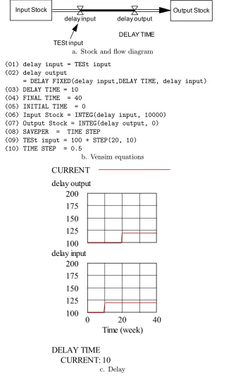
The use of the DELAY FIXED function is illustrated in Figure 6.1. The stock and ¯ow diagram in Figure 6.1a demonstrates a suggested notation for indicating delays in a diagram. In this diagram, there is a delay in the¯ow from Input Stock to Output Stock. The¯ow out of Input Stock is controlled by the

¯ow variable \delay input," and this¯ow enters the delay leading from \delay input" to \delay output," which controls the¯ow into Output Stock. The delay between these two¯ow controls is indicated by a thick solid pipe.

There are three arguments for the DELAY FIXED function, as shown in equation 2 of Figure 6.1b. The rst is the input to the delay, the second is the delay time through the pipeline, and the third speci es what the output should be from the pipeline from the beginning of the simulation until there has been enough time for input to reach the end of the pipeline.

(2)

74 CHAPTER 6 DELAYS, SMOOTHING, AND AVERAGING

DELAY TIME TESt input

Output Stock Input Stock

delay output delay input

a. Stock and¯ow diagram

(01) delay input = TESt input (02) delay output

= DELAY FIXED(delay input,DELAY TIME, delay input) (03) DELAY TIME = 10

(04) FINAL TIME = 40 (05) INITIAL TIME = 0

(06) Input Stock = INTEG(delay input, 10000) (07) Output Stock = INTEG(delay output, 0) (08) SAVEPER = TIME STEP

(09) TESt input = 100 + STEP(20, 10) (10) TIME STEP = 0.5

b. Vensim equations

CURRENT

delay output

200

175

150

125

100

delay input

200

175

150

125

100

0

20

40

Time (week)

DELAY TIME

CURRENT: 10

c. Delay

(3)

from the pipeline will be identical to the input, but delayed by the length of the pipeline.

In some business processes, the length of the delay in a pipeline delay can change depending on conditions elsewhere in the process. For example, the delay in a production process may change depending on the available personnel. If you need to model a situation of this type, then carefully consult the reference manual for your simulation package to be sure you understand what function to use to correctly model such a situation. In particular, you should make sure that the function you use conserves the material in the delay when the delay time changes. In Vensim, the DELAY MATERIAL function should be used for such a situation. This function requires you to specify some information about what happens to material¯ow when the delay changes.

6.2 Third Order Exponential Delays

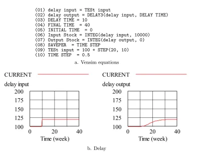
The pipeline delay is an intuitively appealing model for material¯ow delays, but in some situations the ¯ow process is not quite as clearcut. When orders are placed, sometimes all of the ordered goods do not arrive at exactly the same time. That is, there may be some variation in the delay time for the goods to arrive. The third order exponential delay provides a simple model for this situation. The use of this type of delay is illustrated in Figure 6.2. The same stock and¯ow diagram as in Figure 6.1a applies here, but the function for the delay between \delay input" and \delay output" is di°erent than in Figure 6.1. The only change in the information you need to enter is in equation 2, and the modi ed equation is shown in Figure 6.2a.

The third order exponential delay equation in Vensim is called DELAY3, and it has two arguments. The rst is the input variable to the delay, and the second is the delay time through the delay. The initial output from the delay is automatically set equal to the initial input to the delay. (Vensim provides another function DELAY3I which is identical to DELAY3, except that the initial output from the delay can be speci ed as di°erent from the initial input.)

A step input to the third order exponential delay and the resulting output are shown in Figure 6.2b. In the left graph, a step input is shown, and the right graph shows that the output from this changes more gradually than with the pipeline delay. There is very little output for two or three time units after the step occurs, and then the output gradually comes through.

Material¯ow through a third order exponential delay is conserved even if the length of the delay changes while¯ow is occurring.

While the third order exponential delay is a satisfactory way to model many situations where there is some variability in the¯ow rate through the delay, you should be aware that it impacts time-varying inputs in a way that may not be appropriate as a model for some material ¯ow processes. This is illustrated in Figure 6.3.

(4)

76 CHAPTER 6 DELAYS, SMOOTHING, AND AVERAGING

(01) delay input = TESt input

(02) delay output = DELAY3(delay input, DELAY TIME) (03) DELAY TIME = 10

(04) FINAL TIME = 40 (05) INITIAL TIME = 0

(06) Input Stock = INTEG(delay input, 10000) (07) Output Stock = INTEG(delay output, 0) (08) SAVEPER = TIME STEP

(09) TESt input = 100 + STEP(20, 10) (10) TIME STEP = 0.5

a. Vensim equations

CURRENT

delay input

200

175

150

125

100

0

20

40

Time (week)

CURRENT

delay output

200

175

150

125

100

0

20

40

Time (week)

b. Delay

(5)

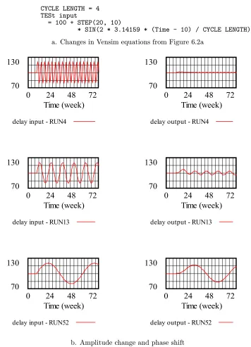
20 starting at time 10. The results for three di°erent cycle lengths (periods) for this sinusoidal are shown in Figure 6.3b. The left hand graphs in Figure 6.3b show the delay input for three di°erent values of CYCLE LENGTH, and the right hand graphs show the resulting delay output for each of these three inputs. Each of the three delay inputs has an amplitude of 20, but the cycle lengths varies. The top curve marked RUN4 has a cycle length of 4 time units, the middle curve marked RUN13 has a cycle length of 13, and the bottom curve marked RUN52 has a cycle length of 52. Thus, if the time units are weeks, these correspond to roughly monthly, quarterly, and annual cycles. Note that the three left hand graphs have the same amplitudes.

However, the amplitudes shown in the output curves in the right hand graphs are substantially di°erent for the three inputs. The amplitude of the graph with a 4 week cycle is so small that it is hard to see much wiggle at all, the graph for the 13 week cycle has a somewhat larger amplitude, and the graph for the 52 week cycle has the largest amplitude. Note that none of these curves has as large an amplitude as the input. Furthermore, each of the output graphs is shifted somewhat to the right from the corresponding input graph. That is, the input is delayed as we would expect. (This delay is sometimes referred to as aphase shift when the input is a sinusoidal curve.)

These graphs illustrate that a third order exponential delay reduces (attenu-ates) inputs which vary over time, and furthermore, it attenuates inputs which vary faster more than inputs which vary slower. Using engineering jargon, a third order exponential delay di°erentially ltersout higher frequency variations, as well asphase shifting the input.

6.3 Information Averaging

Many management actions should not be made in reaction to every random variation in the environment. For example, it takes time and resources to train workers or acquire large capital equipment. You do not want to undertake ma-jor changes in workforce or capital without some assurance that the long term conditions warrant this. In such situations, averaging is used to deal with the inherent irregularity of the processes.

The process of attempting to detect underlying, signi cant changes in data, while ignoring random, transitory¯uctuations is calledaveraging orsmoothing. This process can either be formal using statistical methods, or it can be informal and done \on the¯y" while going about the daily activities of business man-agement. This \psychological smoothing" is widespread, and experience with process models shows that it can have a signi cant impact on the dynamics of a business process. Therefore, it is important to model averaging/smoothing in a process.

(6)

78 CHAPTER 6 DELAYS, SMOOTHING, AND AVERAGING

CYCLE LENGTH = 4 TESt input

= 100 + STEP(20, 10)

* SIN(2 * 3.14159 * (Time - 10) / CYCLE LENGTH)

delay output - RUN52

b. Amplitude change and phase shift

(7)

delayed. The delays in an averaging process can have an important impact on how the process responds to changes in the external environment.

Moving Average

The most obvious averaging procedure is amoving average. With this approach, data is used from a speci ed period (for example, daily sales gures for the last month), and each of the entries used in the average is given the same weight in calculating the average. Thus, the average is calculated by simply adding up the entries and dividing by the number of entries. As time moves along, the average is recalculated by dropping the oldest entry each time period and adding on the most recent entry.

The moving average is a simple procedure to explain and implement. Most people learn how to calculate averages in elementary school, and adding the \moving" component to the procedure is straightforward.

However, this process has one disadvantage, either as a formal calculation procedure, or as a model for the informal averaging that most people do in their heads every day as they take actions. This disadvantage is that the moving average gives the same weight to all of the entries in the average, regardless of how old they are. Thus, if a moving average of daily sales for the last month is calculated, the sales gure for a month ago receives as much weight in calculating the average as the sales gure for yesterday. However, conditions change, and it seems that often the sales gure for yesterday should receive more weight, at least if the average is going to be used as a basis for taking some action. After all, yesterday's sales were made under conditions that are the closest to today's conditions. Especially in a model of how people informally average information, it seems clear that recent data should receive more weight. When we think about past conditions, we are generally give more weight to what has just happened then to conditions days, weeks, or months ago.

Exponential Smoothing

A straightforward averaging process which gives more weight to recent data is

exponential smoothing. With this process, each successively older entry used in the average receives proportionately less weight in calculating the average, and the ratio of the weights for each successive pair of data points is the same. Thus, if the ratio of the weights for the most recent and second most recent data points is 0.8, then the ratio of the weights for any entry and the next older entry will also be 0.8. This implies, for example, that the ratio of the weights between the most recent and the third most recent entries will be 0:8 0:8 = 0:64.

In concept, exponential smoothing considers a set of data stretching back in-nitely far into the past. However, the weights for older data points become smaller as new data points are added, and thus older data points have succes-sively less impact on the average as time goes on.

(8)

80 CHAPTER 6 DELAYS, SMOOTHING, AND AVERAGING

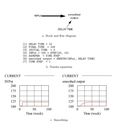
rst of the which is the input to be smoothed, and the second is the averaging constant which is used to set the ratios of the weights for the weighted expo-nential average. Figure 6.4a shows a stock and¯ow diagram for an exponential average. The information arrow over which the averaging is taking place is shown bolder than a standard information arrow. (This notation is useful to quickly show links over which averaging is done, but it is not universally used. In some stock and¯ow diagrams, there is no indication given of a smoothed input.)

Figure 6.4b shows the Vensim equations for the smoothing operation. Equa-tion 7 shows how the smoothing equaEqua-tion is entered.

Figure 6.4c shows the result of smoothing a step input. As we would expect from the discussion above, the smoothed version moves slowly from the original level of the input to the nal level.

The starting value for the SMOOTH output is set equal to the initial value of the input. The function SMOOTHI allows you to set this starting value to a di°erent level if desired.

6.4 Information Delays

(9)

DELAY TIME smoothed

output INPut

a. Stock and¯ow diagram

(1) DELAY TIME = 10 (2) FINAL TIME = 100 (3) INITIAL TIME = 0

(4) INPut = 100 + STEP(20, 10) (5) SAVEPER = TIME STEP

(6) smoothed output = SMOOTH(INPut, DELAY TIME) (7) TIME STEP = 1

b. Vensim equations

CURRENT

INPut

200

175

150

125

100

0

50

100

Time (week)

CURRENT

smoothed output

200

175

150

125

100

0

50

100

Time (week)

c. Smoothing

(10)