Structural and Collaborative Properties of
Team Science Networks
Minh X. Hoang
∗, Ram Ramanathan
†, Terrence J. Moore
‡and Ananthram Swami
‡ ∗Department of Computer Science, University of California, Santa Barbara. Santa Barbara, CA 93106.Email: [email protected]
†Raytheon BBN Technologies, 10 Moulton St, Cambridge, MA. Tel: (617) 873-2736. Email: [email protected] ‡Army Research Laboratory
Email:{terrence.j.moore.civ, ananthram.swami.civ}@mail.mil
Abstract—Team science is a collaborative approach to research, typically with researchers drawn from different disciplines. Team science networks have certain unique characteristics in their conception and intent that set them apart from other commonly studied social and collaboration networks. We study the structural properties, and present metrics for collaborative performance assessment in two real-world team science networks initiated by the Army Research Lab. We model a team using a higher-order generalization of an edge called asimplex. A simplex captures group relationships distinct from the union of pair-wise relationships. Our evaluation using a rigorous methodology reveals that the distributions of vertex and facet degrees (the number of maximal groups that a vertex belongs to) follow a power law, but with exponential cut-off at the tail in most cases. We propose metrics for quantitatively assessing the extent of intra-team and extra-team collaborations, and compare their effectiveness vis-a-vis our intuitive notions. Our work can be used as the basis for generative models, and for evaluating the collaborative performance of team science networks.
I. INTRODUCTION
A social collaboration network is a set of people who interact with each other by means of certain collaborative acts. Examples include publication co-authorship, movie collabora-tions and teams in organizacollabora-tions. The analysis of the structural and evolutionary properties of collaboration networks has been the subject of considerable research over the past decade [1], [2], [3], [4], [5], [6].
We consider a specific type of collaboration network called ateam science network. According to [7], “Team science has been described as a collaborative and often cross-disciplinary approach to scientific inquiry that draws researchers who oth-erwise work independently or as co-investigators on smaller-scale projects into collaborative centers and groups”. Increas-ingly, the hardest problems today require the combined effort of scientists from different fields. Thus, there has been a surge of interest and investment in team science programs by several public agencies such as NIH, NCI, NCCR, ARL, and other private foundations. It is therefore imperative that we understand the structural and collaborative aspects of team science networks.
Team science networks have certain unique features that set them apart from the more typical and well-studied collabora-tion networks such as co-authorship and movie networks. First, unlike the latter networks which are formed by independent
decisions of the actors without an overarching management, team science networks are almost always created by an agency. Second, team science networks are often lightly managed to encourage collaboration between researchers of specific backgrounds, which constrains team formation, but is not as rigid as in business organizational teams. Finally, the structure of actual collaboration in terms of, say, papers co-written, may be different from the team structure.
We investigate two broad questions regarding team science networks: Do topological properties such as degree distribution carry over from other studied collaboration networks (such as co-authorship or movie networks) to team science networks? Given that the main reason for team science is the cross-disciplinary interaction, is there a quantitative way to measure whether such interaction is happening?
Collaboration networks are typically modeled by graphs [8]. However, as recently argued in [9], graphs can only capture pairwise relationships, but are ill-equipped to capture group aspects underlying teams and other other collaborations. For example, consider a complete graph on 4 vertices that repre-sent four people. Does this graph reprerepre-sent a single team of four, four 3-member teams, or six 2-member teams? For such situations, we need an abstraction where higher-order (group) aggregation is a primitive.
In this paper, we represent each collaborator (team member) by a vertex. A set of members who are in the same team is called a simplex. A simplex represents the relation “is in the same team” and thus every team, as well as every possible sub-team, is a simplex. Thus, a team science network is a set of possibly overlapping simplexes (or simplices). A simplex generalizes the notion of an edge, which is a set of cardinality 2, to arbitrary cardinality sets. Similar to the way a weight can be attached to an edge in graphs to represent, say, the strength of a tie, a simplex may beweightedto denote some aspect of the larger aggregation. We provide more detailed and formal definitions in section II.
the Army Research Laboratory (ARL): the Network Sci-ence Collaborative Technology Alliance (NS-CTA), and the Communications and Networking Collaborative Technology Alliance (CN-CTA). Our contributions are as follows:
1) Using rigorous techniques developed in [10], we inves-tigate the fit ofpower lawto the distributions of vertex and facet degree (defined later) in the NS-CTA and CN-CTA, and show that a majority of them follow a power law with exponential cut-off.
2) We propose a metric called the independence ratio to measure the amount of simplex overlap, and compare the independence ratios of NS-CTA and CN-CTA. 3) We devise metrics to evaluate the collaboration level,
both within a team, and between a team and other researchers. We apply these metrics to CN-CTA and NS-CTA to examine the effectiveness of these metrics, and provide an assessment of when and which metric to use.
The remainder of the paper is organized as follows. After introducing the terminologies and the datasets, in section IV, we study two structural aspects of the NS-CTA and CN-CTA. Section V presents metrics for assessing collaboration in team science networks and evaluates them on our two data sets. Related work is discussed in section VI, and we conclude in section VII.
II. REPRESENTINGGROUPS
The use of graphs for representing collaboration networks in general and team science networks in particular does not capture the notion of groups, that is, a set of people working together. We therefore turn to using higher-order aggregations. A team science network is represented as (V, S), whereV is a set of vertices andS is a set of subsetssof V such that all elements ofscollaborate in the same team. Each such subsets is called asimplex1. Any subset of a simplex is also a simplex.
This captures nested sub-teams in a natural fashion, an aspect that will come in handy for assessing intra-team collaboration as a function of the output of sub-teams (section V-A).
A non-empty subset of a simplex sis calledfaceofs. The dimensionof a simplex is one less than the number of vertices in it. Since these simplices can overlap or contain each other, we use the term facet to refer to a maximal simplex, i.e. a simplex that is not a subset of any other simplices. The facet size of a facet is the number of vertices comprising that facet. Similar tovertex degree, which is the number of edges incident to a vertex, thefacet degreeof a vertex is the number of facets that the vertex is a part of. For example, in a social network, the facet degree of a person is the number of maximal groups this person is in. In addition, a minimal non-face (MNF) is a set of vertices such that every subset except the set itself is a simplex. If an MNF has k+ 1 vertices, it is called a k -minimal non-face (k-MNF). The use of these mathematical terminologies allows us to use other related concepts such as “face” and “MNF”, eases the description in section V-A,
1We borrow this and related terminologies later on from mathematics where
it is used in a number of contexts to capture higher-order aggregations.
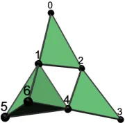
Fig. 1. An example of collaboration network.
and facilitates future work building upon this paper that might leverage other metrics from the field of algebraic topology.
Figure 1 shows a simple collaboration network with three teams:{0, 1, 2},{2, 3, 4}, and{1, 4, 5, 6}. The facet (team) sizes are 3, 3 and 4 respectively, and their dimensions are 2, 2, and 3 respectively. All subsets of the facets, including the facets themselves, are simplices and are shaded. The facet degree of vertex 4 (number of teams it belongs to) is 2 and that of vertex 5 is 1. Note that{1, 2, 4}is not a simplex even though{1, 2}, {1, 4} and{2, 4} are simplices. Instead, {1, 2, 4} is a 2-MNF. MNFs may be used to identify “missed” collaborations. Vertices 1, 2 and 4 are all collaborating pair-wise, which suggests a possible match in their interests. However, they miss an opportunity to combine their skills in a 3-way collaboration. A traditional graph-based model will fail to discern MNFs.
Finally, each simplex in a collaboration network can be assigned a label, indicating certain properties depending on specific problems. An example will be illustrated in the datasets we examine in the next section.
III. DATASETS
We study two real-world team science networks provided by the Army Research Laboratory:
1) NS-CTA: The ARL Network Science Collaborative Tech-nology Alliance (NS-CTA) is an ongoing program study-ing multi-genre networks [11]. The program is currently in its fourth year. In this paper, we work with data from the first three years of this program, including 599 publications from 631 authors. This paper itself is based on work that is part of the NS-CTA.
2) CN-CTA: The ARL Communications and Networking Collaborative Technology Alliance (CN-CTA) was a research consortium for the purposes of developing advanced communications for the military. The program ran from fiscal year 2002 to 2009 and produced a total of 960 publications by 518 authors.
TABLE I
STATISTICS FORNS-CTAANDCN-CTATEAM SCIENCE NETWORKS. GC*STANDS FORGIANTCOMPONENT.
NS-CTA CN-CTA Metrics Team Paper Team Paper Number of vertices 109 631 148 518 Number of edges 871 2133 1536 1248 Max vertex degree 50 143 76 68 Average vertex degree 15.98 6.76 20.76 4.82
Num Components 2 11 1 16
%vertices in GC 96.3 87.0 100.0 87.5
Diameter of GC* 5 9 5 12
Number of facets 77 324 56 341 Max facet size 16 11 22 10 Average facet size 5.45 4.38 9.77 3.31 Max facet degree 13 66 22 62 Average facet degree 3.85 2.25 3.70 2.18 Number of 2-MNFs 789 139 577 51
We extract two collaboration networks from each of the above team science networks: a team network, and a paper co-authoring network. More specifically the team network captures the organization of researchers into the official teams. Each researcher is represented as a vertex, and a set of vertices forms a simplex if and only if the corresponding researchers are in the same team. On the other hand, the paper co-authoring network reflects the collaboration in terms of publishing. In this case, each researcher is still a vertex, but a set of vertices forms a simplex if and only if the cor-responding researchers were co-authors on a published paper. Additionally, for the team network, each simplex is assigned a weight, which is the number of papers that the corresponding researchers co-authored together. From this point, we refer to the team network and paper network extracted from NS-CTA and CN-CTA as NSTeam, NSPaper, CNTeam and CNPaper respectively.
In the team networks, the facet degree of a vertex is the number of maximal teams that the corresponding researcher is a part of. For the paper networks, this is the number of distinct publication collaborations that the researcher participates in. Note that the facet degree for the paper network does not simply count thetotalnumber of papers written by the author, i.e., we don’t add up the weights.
IV. STRUCTURALPROPERTIES
As mentioned in section I, team science networks are unique in the way they are organized and evolve, such as the incentivization for diversity and light management. These factors are likely different for the team network and the paper network. In this section, taking the NS-CTA and CN-CTA as case studies, we investigate the structural properties of team and paper networks.
A. Overview of metrics for NS-CTA and CN-CTA networks
Table I summarizes the statistics of the NS-CTA and CN-CTA team and paper networks. The first set of rows shows traditional graph theoretic metrics and the second set of rows shows group-based metrics in terms of facets and MNFs.
In both CTAs, the paper networks are 5-6 times larger than the corresponding team networks. This is because the paper
networks also include non-CTA collaborators who are not part of the team networks. It appears that the paper networks are far more “spread out” than the team networks. This is indicated by significantly lower average vertex and facet degrees in the paper network, indicating less clustering, as well as significantly higher diameters and numbers of components. This could be due to the fact that the paper network has a bigger element of self-organization, and a large number of non-CTA members, bringing in a flavor of a general co-authorship networks like DBLP.
Recall that a 2-Minimal Non Face (2-MNF) is a set of verticessof cardinality 3 such that every subset ofsexcepts itself is a simplex. One interesting question is if the number of 2-MNFs are more dependent on network size, vertex degree or facet degree. Evidence from Table I indicates more support for the latter two. If we compare the 4 sets (NSTeam vs. CNTeam), (NSPaper vs. CNPaper), (NSTeam vs. NSPaper), and (CNTeam vs. CNPaper), we see that the number of 2-MNFs increases with increasing size for only one of them. Whereas, the number of 2-MNFs increases with increasing average vertex degree for 3 of them and with average facet degree for all four. It appears that the more tightly packed a network is, the more chances exist for a 2-MNF.
From the above, it appears that the team and paper networks, while comprising many same researchers, are somewhat dif-ferent in their collaborative phenomena. One reason could be that the team networks were formed with some amount of management and incentivization, whereas the paper networks are drawn from pre-existing informal relationships prior to the team formation.
B. Vertex and Facet Degrees: Power Law?
A remarkable feature of many natural phenomena is that the vertex degrees are power law distributed [10]. We now investigate if this property holds for team science networks, and whether it extends to facet degrees.
We adopt the rigorous method proposed by Clauset et al. [10] to decide if a distribution follows power law. Given a variablex, this method fits the complementary cumulative dis-tribution function (CCDF) of the data to the Pareto cumulative distributionP[X≥x]∝xγ, which is analogous to power law distribution. If plotted in a log-log scale, this distribution will appear as a straight line. We will report two parameters of the fitting obtained by their method: the exponent γ, andxmin. Since the power-law distribution often does not hold for the entire range of data, in particular not for smaller values,xmin is the smallest values of the corresponding variable x upon which the straight line power-law form still asserts itself.
100 101 102
Vertex Degree 10-3
10-2
10-1
100
CCDF
(a) NSTeam VD
100 101 102
Facet Degree 10-3
10-2
10-1
100
CCDF
(b) NSTeam FD
100 101 102 103
Vertex Degree 10-3
10-2
10-1
100
CCDF
(c) NSPaper VD
100 101 102
Facet Degree 10-3
10-2
10-1
100
CCDF
(d) NSPaper FD
100 101 102
Vertex Degree 10-3
10-2
10-1
100
CCDF
(e) CNTeam VD
100 101 102
Facet Degree 10-3
10-2
10-1
100
CCDF
(f) CNTeam FD
100 101 102
Vertex Degree 10-3
10-2
10-1
100
CCDF
(g) CNPaper VD
100 101 102
Facet Degree 10-3
10-2
10-1
100
CCDF
(h) CNPaper FD
Fig. 2. Vertex degree (VD) and facet degree (FD) distributions of NS-CTA and CN-CTA paper and team networks
TABLE II
POWER LAW FITTING AND LIKELIHOOD RATIO TEST RESULTS FORNS-CTAANDCN-CTA
Dataset Power Law Poisson Log-normal Exponential Stretched exp. Power law + cut-off Support for
xmin γ p LR p LR p LR p LR p LR p power law
NSTeam VD 23±4 5.1±0.9 0.10 5.3 0.33 -0.9 0.44 -1.0 0.28 1.0 0.70 -1.0 0.15 good NSTeam FD 5±1 3±1 0.07 -2.4 0.41 -2.9 0.12 -2.7 0.02 -3.0 0.04 -2.9 0.02 with cut-off NSPaper VD 5±1 2.6±0.2 0.14 654 0.01 -2.5 0.21 30.6 0.08 33.7 0.06 -2.7 0.02 with cut-off NSPaper FD 1.0±0.8 2.2±0.2 0.01 516 0.00 -5.7 0.02 104 0.00 -3.6 0.32 -6.1 0.00 with cut-off CNTeam VD 19±3 3.2±0.3 0.05 133 0.05 -186 0.00 -157 0.00 -182 0.00 -183 0.00 with cut-off CNTeam FD 4.0±0.7 2.9±0.3 0.18 24.4 0.36 -35.6 0.00 -37.0 0.00 -37.0 0.00 -37.0 0.00 with cut-off CNPaper VD 6±1 3.0±0.2 0.58 275 0.04 -207 0.00 -179 0.00 -179 0.00 -179 0.00 with cut-off CNPaper FD 1.0±0.4 2.2±0.1 0.23 441 0.01 -3.4 0.09 94.9 0.00 1.7 0.72 -3.4 0.01 with cut-off
law distribution with an exponential cutoff has the following form:
P(z)∝x−γe−x/xc,
where γ and xc are constants, and x is the variable in consideration, i.e., vertex or facet degree in our case.
The distributions of vertex degree (VD) and facet degree (FD) of NS-CTA and CN-CTA networks vis-a-vis a power law distribution are depicted in Figure 2. The fitting parame-ters for power law and the likelihood ratio test to compare power law distribution with other distributions are shown in Table II. p-values are bolded in cases the corresponding tests are considered statistically significant: p-values greater than 0.1 for power law fitting, and less than 0.1 for log likelihood ratio tests [10]. If the log-likelihood ratios are positive, then the power-law model is favored over the al-ternatives. The last column lists judgment of the statistical support for the power-law hypothesis. Of the 8 combinations of {vertex-degree, facet-degree} × {team, paper} × { NS-CTA, CN-CTA}, 7 combinations can be deemed as power law with exponential cut off in the tail. One of them, the vertex degree of NSTeam, is a power law fit without cut-off.
For the vertex degree distributions of both NSTeam and CNTeam, the values of xmin are very high (23±4for NSTeam and 19±3 for CNTeam) reducing the dependability of this assessment. However, the facet degree distributions display a power law with cut-off even with our strict methodology. Finally, we note that the two team science networks are quite similar to each other in terms of vertex and facet degree distribution.
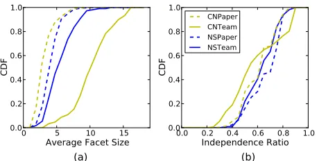
C. Facet Degree and Size
The fact that vertex degrees and facet degrees show some-what different distribution behavior above leads us to investi-gate the overlapamong groups that a person participates in. Note that if there were no overlaps, and all facets were of equal size, then the vertex and facet degrees would correlate almost perfectly. Further, if there were overlaps but all facet sizes were the same, the ratio between the vertex and facet degrees would be a measure of the overlap. Since in real networks, facet sizes are clearly not single-valued, we construct the following new metric to measure the overlap:
0 5 10 15
Average Facet Size
0.0 0.2 0.4 0.6 0.8 1.0
CDF
0.0 0.2 0.4 0.6 0.8 1.0
Independence Ratio
0.0 0.2 0.4 0.6 0.8 1.0
CDF
CNPaper CNTeam NSPaper NSTeam
(a)
(b)
Fig. 3. Cumulative Distribution Function (CDF) of average facet size per vertex and independence ratio for Team Science Networks.
Intuitively, the lower I(v)is, the more facets incident tov overlap, i.e., the less independent the collaborating groups are. This measure is also technically valid for a graph, in which all simplices have dimension of at most one, but is trivial, namely
1
2 for all vertices.
Figure 3 shows the cumulative distribution function (CDF) of the average facet size per vertex and the independence ratio for NS-CTA and CN-CTA networks, which clearly show that the two team science paper networks are similar to each other.
V. METRICS FORASSESSINGCOLLABORATION
While team science networks are formed with the goal of cross-fertilizing ideas from different fields, this in and of itself does not ensure that the members actually work together. Quantifying the level of collaboration within each team to assess if the team is functioning as intended would be valuable for managing team composition and network structure. In order to assess the level of interaction, we need to have an objective measure of the team’s collaborative performance. For team science networks that are the focus of this paper, namely the NS-CTA and the CN-CTA, the number of publications jointly authored by the team members is a reasonable measure of their interactions.
Papers are seldom written by a team as a whole, but more typically by different sub-teams along topics of interest to the particular sub-team. Thus, we need a way to combine the collaborations between arbitrary subsets in the team into an overall assessment of a team’s collaborative performance and, similarly, to assess the collaboration between a team and non-team members. In the remainder of this section, we devise metrics for evaluating the extent of collaboration of a team, both within itself – intra-team collaboration, and with other non-team members – extra-team collaboration.
A. Intra-Team Collaboration
We model each team as a simplex – in particular a facet – with the subset closure property implicit in the definition of the simplex elegantly capturing the sub-team collaborations. Re-call that a non-empty subset of a simplex is termed the face of the simplex. To model the amount of collaboration, each face is assigned a non-negative weight indicating the collaborative performance, e.g., the number of papers published together
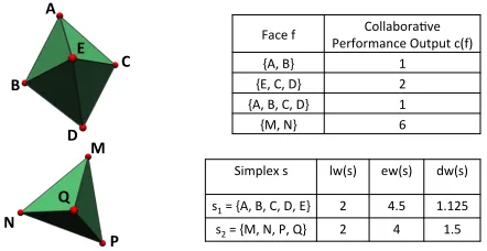
by people in the face, termed the collaborative performance output (CPO) of the face. A higher CPO indicates more collaboration. Note that the CPO is assigned to both facets (teams) as well as non-facet simplices (subsets of teams). If a face of dimension greater than 0 has a positive CPO, we call it a collaborative face. The collaborative faces with largest dimension in a simplex are termed the largest collaborative faces. Figure 4 shows two example facets:s1={A, B, C, D,
E}with 5 vertices ands2={M, N, P, Q}with 4 vertices. The
CPO’s of their collaborative faces are shown in the adjacent top right table.{E,C}, for instance, is not a collaborative face. The largest collaborative faces are{A, B, C, D} with a CPO of 1 fors1, and{M, N} with a CPO of 6 fors2.
We quantify the collaboration among any subset of indi-viduals comprising a team as the collaborative score of the corresponding simplex. The collaborative score of a simplex is defined as a function of the CPO’s of its faces. Although the concept of a collaborative score is applicable to any non-facet simplex (sub-team), we are primarily interested in the collaborative score of a facet (team as a whole). In what follows, we consider the definition of collaborative score.
Let s denote the target simplex whose collaborative score needs to be evaluated. In our case, the simplices being scored are teams from the team datasets, while the paper datasets provide the CPO’s of their faces. Denote byF(s)the set of all collaborative faces, by dim(s) the dimension of s. Let c(k) denote the CPO of a simplex k ⊆ s. We use the following general rules of thumb to devise our metrics. Aspects that merit a higher score include:
1) A higher dimension of the largest collaborative faces in relation to the dimension of the target simplex.
2) The magnitude of collaboration, i.e., the CPO’s of the faces within the target simplex.
We now describe the formulation of our proposed metrics. Each of the metrics biases one aspect over the others, and thus results in different assessment of the collaboration level. Note that the 0-dimensional faces, i.e., faces with a single vertex, do not affect the collaborative score of a simplex. For all metrics, simplices with higher collaborative scores exhibit a higher level of collaboration.
Definition 2: The linearly weighted collaborative score lw(s)of a simplexsis defined as:
lw(s) =
P
k∈F(s)dim(k)∗c(k)
dim(s)
Here, the CPO’s of the collaborative faces are weighted by their corresponding dimensions and normalized by the dimension of the target simplex.
One might argue that larger collaborations require more effort and should be suitably “rewarded” in the score. In the following two metrics, instead of linearly weighting the faces, we weight them by an exponential2function of the dimensions.
2We chose exponential based on our sense that for typical teams the
TABLE III
FIVE SAMPLE TASKS IN THENS-CTA,THEIRCPO’S(PUBLISHED PAPER COUNTS)AND THE SCORES BY EACH OF THE FOUR PROPOSED METRICS.
Team Members Collaborative Faces and CPO’s lw(s) ew(s) dw(s) T1 M01, M02, M03 {M02, M03 : 5} 2.5 5 2.5 T2 M04, M05, M06 {M04, M06 : 4} {M04, M05, M06 : 3} 5 10 5 T3 M07, M08, M09 {M09, M08 : 1} {M09, M07, M08 : 2} 2.5 5 2.5 T4 M10, M11, M12 {M11, M12 : 7} {M10, M12 : 3} 7 14 7
{M11, M10, M12 : 2}
T5 M13, M14, M15, M16 {M18, M13 : 1} {M17, M18 : 2} 3.83 9 0.84 M17, M18, M19 {M16, M15 : 1} {M19, M18 : 3}
{M14, M16, M15 : 2} {M19, M18, M13 : 4} {M14, M16, M19, M18, M15 : 1}
Definition 3: The exponentially weighted collaborative scoreew(s)of a simplexs is defined as:
ew(s) =
P
k∈F(s)2
dim(k)∗c(k)
dim(s)
One problem with ew(s) defined above is that the nor-malization is still linear in dim(s), which tends to favor larger simplices. The following formulation “damps” the score exponentially using a function of the dimensions.
Definition 4: The exponentially damped collaborative score dw(s)of a simplexsis defined as:
dw(s) = X f∈F(s)
2dim(f)−dim(s)∗c(f)
For the example in Figure 4, we have: dim(s1) = 4
and dim(s2) = 3. As can be seen from the bottom right
table of Figure 4, the scoring functions differ on which simplex is deemed the more collaborative. While dw(s) deems (M, N, P, Q) to be more collaborative, ew(s) deems (A, B, C, D, E)to be so, andlw(s)assesses them to be equal. Each metric reflects a different emphasis on the CPO’s – the number of papers – vesus the largest collaborative sub-team and the simplex dimension. We now evaluate these metrics on the team networks of NS-CTA and CN-CTA. While understanding the collaboration within these team science networks is certainly of interest, we also seek to answer the following questions: Which of these metrics match “intuition”? How do these metrics correlate with each other? Are all of the three metrics useful? Which is the best metric for team science networks?
We first assign collaborative performance outputs to the team simplices in each of NS-CTA and CN-CTA. The CPO’s of a simplex in the team network is the number of papers published together by exactly the corresponding members in that team simplex. By “exactly”, we mean that the highest-cardinality matching face is used. In other words, each paper is counted only once, for the maximal intersecting simplex be-tween the paper simplex and the corresponding team simplex. For instance, if A, B, and C publish a paper together, it will only affect the CPO of the simplex {A, B, C}, but not the CPO of any subset or superset of{A, B, C}, such as{A, C},
{B, C},{A, B}, and{A, B, C, D}. We now compute the three metrics defined above for each team as the target simplex.
Table III illustrates each of the metrics for five anonymized sample teams within the NS-CTA. The second column con-tains the identifiers of the team members and the third column shows the CPO of each collaborative face in the team. The fourth column contains the largest collaborative dimension, followed by the three metrics lw(s), ew(s), and dw(s). For each metric, we look at the rankings of the teams and consider if it matches our “intuition”. All three metrics rank T4 and T2 as the most and second-most collaborative respectively. However,dw(s)differs sharply in its evaluation of T5, which it rates last. This is because T5 is a high-dimensional group, and thus is penalized bydw(s).
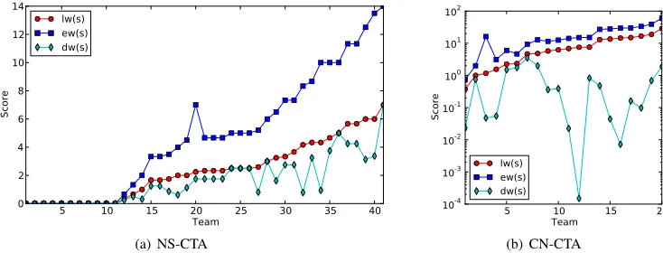
A complete picture of the relative values of the collaborative scores for all teams in NS-CTA and CN-CTA is shown in Figure 5. The teams on the x-axis are sorted in increasing order oflw(s). Comparing the metrics, it can be seen thatlw(s)and ew(s)“track” together, more or less, in the NS-CTA as well as CN-CTA. For the sample teams in Table III, the rankings based on these two metrics are also the same (modulo tie breaking). To confirm this, we run a Spearman’s correlation evaluation on these metrics. We observe a clear similarity betweenew(s) andlw(s)with correlation coefficients of 0.99 (NS-CTA) and 0.84 (CN-CTA). Whetherew(s)orlw(s)is “better” depends upon how much value we give to higher-order collaborations. In our experience with team science research, the difficulty of collaboration between scientists (who are typically strongly opinionated!) does increase quite rapidly with size of the team. Thus, we recommendew(s)overlw(s), i.e., we want to
super-A
B
C
E Face f
Collabora,ve Performance Output c(f)
{A, B} 1
{E, C, D} 2
{A, B, C, D} 1
{M, N} 6
D M
N
P Q
Simplex s lw(s) ew(s) dw(s)
s1 = {A, B, C, D, E} 2 4.5 1.125
s2 = {M, N, P, Q} 2 4 1.5
5 10 15 20 25 30 35 40 Team
0 2 4 6 8 10 12 14
Score
lw(s) ew(s) dw(s)
(a) NS-CTA
5 10 15 20
Team
10-4
10-3
10-2
10-1
100
101
102
Score
lw(s) ew(s) dw(s)
(b) CN-CTA
Fig. 5. Collaborative scores across teams for each of the metrics, with a view to discern correspondence in behavior.
linearly reward higher-order collaborations.
In summary, we propose thatew(s)anddw(s)be used for evaluations. If the researchers have a lot of latitude in forming teams, and the alliance coordinators want to dissuade having members who are part of the team but hardly collaborate in papers, then dw(s)should be used. On the other hand if the teams have been intentionally put together by the alliance coordinators, it does not make sense to penalize larger teams. Hence, ew(s)should be preferred.
B. Extra-team Collaboration
A healthy collaboration profile should balance the number of collaborations with an individual, and the number of indi-viduals with whom one has collaborated. In order to devise a metric for this purpose, we borrow from the popular concept ofH-index[12], which is defined as follows: an author has an H-index ofhif he/she has publishedhpapers, each of which has been cited in other papers at least h times. In a similar way, we define thecollaboration index, orc-indexas follows: Definition 5: A simplex T has a c-index c if there are at leastcnon-simplex members, each of whom have collaborated with at least one member of T at leastc times.
The above definition easily instantiates to the case of an individual, which we shall refer to as vertexc-index. In other words, an individual has a vertexc-indexcif there are at least c other individuals each of whom have collaborated with the individual at least ctimes.
We now evaluate these metrics on the NS-CTA and CN-CTA networks. Instead of all possible simplicies (sub-teams), we focus on the vertex (individual) and the team as organized officially in these two organizations. To compute the c-index of a vertex, we create an induced network from the paper dataset while using only the people present in the team dataset, i.e. only people officially in the NS-CTA and CN-CTA. For each person, we sort all of his/her neighbor vertices who have published at least a paper with him/her in decreasing order of the strength of collaboration between them–the edge weight– which is literally the number of common papers. The c-index of the corresponding vertex will be computed based on this sorted list of edge weights with respect to definition 5. Thec -index of a team is computed similarly. Further, we normalize
each team’sc-index by the team size because c-index counts the collaborations with at least one member and hence by definition would be higher for larger team sizes.
Figure 6 shows the distribution of vertex c-index and normalized team c-index for NS-CTA and CN-CTA. These distributions are remarkably similar between the two networks. Given such similarity between two team science networks, we wonder if it might be that extra-team collaboration in team science networks has a certain “signature” in the way the collaborations are distributed. More data sets need to be analyzed to confirm this, but if so, it would provide a way to distinguish “anomalous” team science collaborations.
Finally, while there is a clear relationship between the vertex and facet degrees with Spearman’s correlation coefficients greater than 0.82, there is no clear indication of such rela-tionship between c-index and either vertex or facet degree. However, we observed that the person who ranks the highest in the number of collaborations also ranks the highest in vertex c-index, in both the NS-CTA and CN-CTA.
VI. RELATEDWORK
The last decade has seen a spurt in the study of collaboration networks. In [1], [2], structural properties of publicly available scientific publication networks are analyzed, with the latter also investigating evolutionary aspects. Self-organization and classification into different kinds of small-world networks
0 1 2 3 4 5 6 7
Vertex C-index
0.0 0.2 0.4 0.6 0.8 1.0
CDF
0.0 0.2 0.4 0.6 0.8 1.0 1.2 1.4 1.6
Normalized Team C-Index
0.0 0.2 0.4 0.6 0.8 1.0
CDF
NS-CTA CN-CTA
(a)
(b)
appear in [3], [5]. The quest to discern power laws in the distribution of social networks has been the subject of much work in the literature [10], [13]. Visual and other simplistic methods, however, may be misleading [14], [10]. A rigorous method for verifying if a distribution follows power law is given in [10], which we apply in this paper.
The scientific study of team science networks have recently received attention under the banner of ScITs (Science of Team Science) [15], [7]. Team formation has been studied in [16]. A study of the impact of the network structure on the performance of leaders and teams has been reported in [17], [18]. Results suggest that team performance is positively correlated with network density and team centrality. However, to our knowledge, the structural properties and quantitative collaboration performance metrics have not been studied.
Related to our work on collaboration levels is the concept of cohesionin social sciences literature, such as [19]. In contrast to these works, our goal is to assess whether and how well a team is collaborating based on its collaborative output, e.g., by joint analysis of team and paper networks.
Alternate representations for social collaboration networks to capture higher-order relations include the bipartite graph andhypergraph[8]. Our choice of the simplexrepresentation is to reflect the natural closure property in the relation “is in the same team”, and to facilitate future work building upon this paper that might leverage other metrics from the field of algebraic topology.
VII. CONCLUDINGREMARKS
We have studied two real-life team science networks: the ARL NS-CTA and CN-CTA. Using a more general representa-tion than graphs – the simplex – we have analyzed metrics such as facet degree, facet size, independence ratio and minimal non-face in addition to the traditional graph-theoretic metrics. We have shown that the distributions of vertex and facet degrees resemble a power law with exponential cut-off.
We have investigated the problem of assessing intra-team and extra-team collaboration in team science networks and presented metrics for both intra-team and extra-team col-laboration assessment. Evaluating these metrics on the NS-CTA and CN-NS-CTA, we have examined and discussed these results vis-a-vis our intuition. Our analysis has helped provide recommendations on the situation under which each metric would be useful. Moreover, we have seen that the extra-team collaboration profile is remarkably similar in both networks.
The structural properties uncovered in this paper can be used as the basis for generative models of team science networks. Further, our proposed collaborative metrics can be applied to performance evaluation and improvement plan in team science networks.
ACKNOWLEDGMENT
Research was sponsored by the Army Research Laboratory and was accomplished under Cooperative Agreement Number W911NF-09-2-0053. The views and conclusions contained in this document are those of the authors and should not
be interpreted as representing the official policies, either expressed or implied, of the Army Research Laboratory or the U.S. Government. The U.S. Government is authorized to reproduce and distribute reprints for Government purposes notwithstanding any copyright notation here on.
REFERENCES
[1] M. E. J. Newman, “The structure of scientific collaboration networks,”
Proc. National Academy of Sciences, vol. 98, no. 2, pp. 404–409, 2001. [2] A. Barabˆasi, H. Jeong, Z. N´eda, E. Ravasz, A. Schubert, and T. Vicsek, “Evolution of the social network of scientific collaborations,”Physica A: Statistical Mechanics and its Applications, vol. 311, no. 3, pp. 590–614, 2002.
[3] J. J. Ramasco, S. N. Dorogovtsev, and R. Pastor-Satorras, “Self-organization of collaboration networks,” Phys. Rev. E, vol. 70, no. 3, Sep 2004.
[4] P. Zhang, K. Chen, Y. He, T. Zhou, B. Su, Y. Jin, Y. Chang, H. an d Zhou, L. Sun, B. Wang et al., “Model and empirical study on some collaboration networks,”Physica A: Statistical Mechanics and its applications, vol. 360, no. 2, pp. 599–616, 2006.
[5] L. Amaral, A. Scala, M. Barth´el´emy, and H. Stanley, “Classes of small-world networks,” Proceedings of the National Academy of Sciences, vol. 97, no. 21, pp. 11 149–11 152, 2000.
[6] M. Franceschet, “Collaboration in computer science: A network science approach,”Journal of the American Society for Information Science and Technology, vol. 62, no. 10, pp. 1992–2012, 2011.
[7] L. Bennett, H. Gadlin, and S. Levine-Finley, “Collaboration and team science: A field guide,” Bethesda, MD: National Institutes of Health, 2010.
[8] S. Wasserman and K. Faust, Social network analysis: Methods and applications. Cambridge university press, 1994, vol. 8.
[9] R. Ramanathan, A. Bar-Noy, P. Basu, M. Johnson, W. Ren, A. Swami, and Q. Zhao, “Beyond graphs: Capturing groups in networks,” inProc. IEEE NetSciComm. IEEE, 2011, pp. 870–875.
[10] A. Clauset, C. Shalizi, and M. E. J. Newman, “Power-law distributions in empirical data,”SIAM review, vol. 51, no. 4, pp. 661–703, 2009. [11] “The Network Science CTA, http://www.ns-cta.org/.”
[12] J. Hirsch, “An index to quantify an individual’s scientific research output,”Proceedings of the National Academy of Sciences of the United states of America, vol. 102, no. 46, p. 16569, 2005.
[13] M. E. J. Newman, “Power laws, pareto distributions and zipf’s law,”
Contemporary physics, vol. 46, no. 5, pp. 323–351, 2005.
[14] M. Goldstein, S. Morris, and G. Yen, “Problems with fitting to the power-law distribution,”The European Physical Journal B-Condensed Matter and Complex Systems, vol. 41, no. 2, pp. 255–258, 2004. [15] D. Stokols, K. L. Hall, B. K. Taylor, and R. P. Moser, “The science of
team science: overview of the field and introduction to the supplement ”
Am J Prevent Med, vol. 35, no. 25, pp. 77–89, 2008.
[16] T. Lappas, K. Liu, and E. Terzi, “Finding a team of experts in social networks,” in Proceedings of the 15th ACM SIGKDD international conference on Knowledge discovery and data mining. ACM, 2009, pp. 467–476.
[17] R. T. Sparrowe, R. C. Liden, S. J. Wayne, and M. L. Kraimer, “Social networks and the performance of individuals and groups.”Academy of management journal, vol. 44, no. 2, pp. 316–325, 2001.
[18] P. Balkundi and D. A. Harrison, “Ties, leaders, and time in teams: Strong inference about network structure’s effects on team viability and performance.”Academy of Management Journal, vol. 49, no. 1, pp. 49– 68, 2006.