Multivariate Analysis of Data on the Effects of Different Vegetative Covers on Some Physical Properties of a Selected Nigerian Soil

(1)

2013; 2(6): 210-220

Published online November 10, 2013 (http://www.sciencepublishinggroup.com/j/ajtas) doi: 10.11648/j.ajtas.20130206.18

Multivariate analysis of data on the effects of different

vegetative covers on some physical properties of a

selected Nigerian soil

CHUKWUDI JUSTIN OGBONNA

1

, OPARA JUDE

2

, HYCINTH CHUKWUDI IWU

1

1_{Federal University of Technology Owerri Nigeria PMB 1526, Owerri Nigeria} 2_{Department of Statistics, Imo State University PMB 2000, Owerri Nigeria}

Email address:

[email protected](C. J. OGBONNA), [email protected](J. OPARA), [email protected](H. C. IWU)

To cite this article:

CHUKWUDI JUSTIN OGBONNA, OPARA JUDE, HYCINTH CHUKWUDI IWU. Multivariate Analysis of Data on the Effects of Different Vegetative Covers on Some Physical Properties of a Selected Nigerian Soil.American Journal of Theoretical and Applied Statistics. Vol. 2, No. 6, 2013, pp. 210-220. doi: 10.11648/j.ajtas.20130206.18

Abstract:

This work discusses the use of multivariate analysis of variance to tackle the problem of investigating the effects of different vegetative covers on the physical properties of a selected Nigerian soil. An additive effect model was assumed and using data obtained from the Department of Soil Science of the University of Nigeria, Nsukka, we tested for the equality of significant treatment effects. The result of the analysis revealed that the treatment effects were found to be significant being acceptable at 5 percent level. Based on our analysis, we recommended that the vegetative covers in question are useful and necessary and therefore should be used to improve the soil physical conditions for any overused land in Nsukka area of Nigeria and similar soils elsewhere not in Nsukka depending on the use and type of farming system the land is put to.

Keywords

:

RCBD, MANOVA, Vegetative Covers

1. Introduction

In recent times, a lot of ways and means of increasing agricultural products for food fiber have been sought for. This is to increase food to feed the increasing population; the Mohammed/Obasanjo regime introduced “The Operation Feed the Nation” programme. The ousted Alhaji Shehu Shagari regime christened the same effort of increasing food production, “The Green Revolution”. And more recently, the administration of Yar’adua and Goodluck Ebele Jonathan put up spirited efforts to secure food security for the nation. This is primarily agrarian based, emphasizing on the development of modern technology, research, financial injection into research, production and development of agricultural inputs to revolutionalise the agricultural sector leading to a 5–10 fold increase in yield and production. This will result in massive domestic and commercial outputs and technological knowledge transfer to farmers. To achieve this aim of providing adequate food for the teeming population as well as materials for the agro-based industries, it becomes imperative to study the soil on which the food and raw materials are to be grown.

The soil is the medium where plants grow. It provides environment for germination, development and plants roots development. It is a three phase system comprising solid, liquid and gaseous phases. These phases have been so much disturbed by traditional practices of farming resulting, for instance, in vegetative degradation. Vegetative degradation is regarded as a reduction in the available biomass, and decline in vegetative ground cover. It may result from deforestation and overgrazing. Such degradation particularly causes soil erosion and loss of soil organic matter that we cannot over gainsay the need to improve the soil condition.

(2)

Combating vegetation degradation either through natural grassland or planted crops has the potential to contribute directly to the maintenance and improvement of soil productivity. Vegetation covers protect the soil from intense precipitation of rain and detachability of surface materials. It reduces runoff, conserved the moisture and retains sediment and organic debris. It also allows drainage of excess water due to their semi-permeable nature.

Conventional tillage which creates favorable environment for crop growth, can also damage pore continuity and promote dispersion of clay forming crust and create dense, non-friable clods and aggregates. Soil water status affects soil properties either directly by its influence on soil weathering and profile development or indirectly on a short term basics by influencing soil factors such as soil strength, friability and permeability to water and solutes and gases. Unfortunately, most interest in soil water is centered on its content and availability with little or no regards for its interrelations with other soil properties and environmental factors. The importance of maintaining or improving the soil physical properties in agriculture has been reported by a lot of soil researchers; See for example Enyioko et al (2012), Amana et al (2011), Egwuatu (1982), etc.

The ultimate objective of this study is, therefore, to use multivariate analysis of variance to investigate the effects of vegetative covers on some physical properties of a selected Nsukka soil as well as the interrelationships of the physical properties of the soil measured. Specifically the study:

(i) evaluated the data to test if there are significant differences of the effects of different vegetative covers on the physical properties of the soil measured, and

(ii) estimated the effects of such vegetative covers on the soil that are found statistically significant.

2. Definition of Terms

• Infiltration rate of water into the soil: this is defined as the entry rate of water into the soil from infiltrometer and denotes both horizontal and vertical components of flow in the soil. It is the downward component of flow which is of more interest for a study of rainfall hydraulic.

• Hydraulic conductivity: this is the readiness with which water flows through the soil in response to a given gradient.

• Moisture content of the soil: this is the measure of the ability of the soil to retain water which is always available to the plants for use.

• Bulk density: the bulk density of a soil is the ratio of its weight to the weight of the same volume of water. The higher the bulk density of a soil the less the pore spaces in the soil.

• Particle density: this is the weight per unit volume of a soil.

• Porosity of the soil: the spaces left in between

particles of a soil sample are called pores. The relative volume of pores to solid material is called the total pore space or total porosity. These spaces permit air and water to move in the soil. They also allow soil organisms and plant roots free movement in the soil. The porosity of a soil therefore has an important part to play in the suitability of the sample for agricultural purposes when the pore spaces are large they are called air-spaces but when they are very small, they are called capillary pore spaces.

• Soil texture: this refers to the proportion or percentage of the sample e.g. sandy soil, coarse soil and clay soil. This proportion of the various sizes in a soil sample has important effects on the soils physical and chemical properties.

3. Literature Review

Enyioko et al (2012) carried out a research work on Soil Characteristics and structural stability of a Typic Paleustult under Different Vegetation Cover. The different cover management practices were bare fallow (BF), cassava cultivation (CS), groundnut cover (GN), manured groundnut cover (GN + PM) and Panicum maximum (PMC), while the soil properties studied were water drop energy (impact), macro porosity, micro porosity, saturated hydraulic conductivity, soil moisture content at 6kpa, soil aggregate stability, and penetration resistance. Data were subjected to analysis of variance using RCBD, and results show that soil resistance to penetration was highest in the bare fallow treatment (1.7kg/m2) and lowest under the manured groundnut treatment (1.0kg/m2), soil total porosity and macro porosity were highest (50.84 and 24.4% respectively) under the manured groundnut treatment and lowest (43.16 and 16% respectively) under the cassava plot. Saturated hydraulic conductivity was lowest in the cassava plot (23.3cm/h) but highest in the manured groundnut plot. The management practices aggregates to pass through a 4.75mm sieve. The highest drop number and energy values were obtained for aggregates formed under Panicum cover whereas the lowest values were obtained for aggregates of the bare soil. The percent aggregate stability > 0.5 was not statistically significant but was highest for the Panicum maximum treatment closely followed by the bare fallow treatment and GN + PM treatment. The overall trend in changes in soil water properties (Ksat, PT, and macro-porosity) was BF ≤ CS < GN < PMC < GN + PM.

(3)

change in soil texture due to treatments. The treatments generally increased organic matter content compared with the control. Bulk density was significantly increased in all the treatments with highest value (1.65Mg/m3) in bare fallow and lowest value (1.49 Mg/m3) in grass. There was no significant decrease in porosity and pore size distribution. Mean weight diameter (MWD) of aggregates and saturated hydraulic conductivity (Ksat) were significantly increased. The least values for MWD (1.06mm) and for Ksat (25.80cm/hr) and highest for MWD (2.09mm) and for Ksat (49.20cm/hr) were obtained under bare fallow and grass treatments respectively. The percentage aggregate size above 2.0mm was highest in grass and lowest in bare fallow. Calculations showed significant positive correlation (r = 0.50) between organic matter and MWD. There was significant negative correlations (r = -0.60) between organic matter and bulk density and highly significant positive correlation (r = 0.800) between organic matter and saturated hydraulic conductivity.

Egwuatu (1982) studied the effects of different ground covers on the physical properties of Npologu series (sandy, clay and loam). The ground covers were fallow, original, cover, stylosanthes, peuraria, creeping cover, guinea and carpet covers. The properties he studied were texture, porosity and pore size distribution, aggregate stability and infiltration capacity of the soil. After a univariate analysis of his observations using two-way Analysis of Variance he came out with the following result: that the effects of the different vegetative covers on Nsukka sandy clay loam soil indicated that the covers did not significantly influence the soil texture and total porosity while they significantly affected the infiltration capacity of the soil.

Soil characteristics such as infiltration, saturated hydraulic conductivity, soil porosity, and water retention and availability has been related to soil structure. Research works (Wood et al, 1987) relating soil infiltration characteristics to land use for instance found that ground cover control infiltration, while Lugo Lopez et al. (1981) reported that infiltration is a function of soil properties such as bulk density, pore size distribution and aggregate stability. According to Adeoye (1982), deep tillage of Alfisol in Norther Nigerian result in increased porosity, while Tollner et al (1984) reported that beneficial effects of tillage on soil include an increase in the number of drainage pores in the soil. According to Papendick and Campell (1981), water retention in soils is influenced by texture, organic matter content and the physical composition of the soil. Soil with high amount of clay content and organic matter for instance hold considerably more gravimetric water at a given water potential than soil with a high content of sand. Also, Mabgwu and Ekwealor (1990) reported high moisture retention for different soils amended with brewer’s spent grain, while Mbagwu (1989) reported that addition of organic matter at any rate significantly increased soil water retention except at 1.500kpa. However, for exposed soils especially highly degraded soils in the

tropics water retention is reduced and this is attributable to runoff and possibly a reduction in porosity due to high bulk density.

In this study, we use multivariate analysis of variance to investigate the effects of different vegetative covers on some physical properties of a selected Nsukka soil. We shall also try to identify the various treatment effects found statistically significant for the studied variables.

3. Experimental Design/Methodology

3.1. Data

The data used for this study are secondary data collected from undisturbed soil samples which were collected two days after it had rained from the University of Nigeria, Nsukka Agricultural Experimental Field where the research was conducted and then subjected to mechanical and physical analysis in the soil science laboratory of Department of Soil Science, University of Nigeria, Nsukka. It should be noted that the undisturbed soil samples were removed from each experimental unit.

The design was a randomized complete block design with the experiment arranged in four randomized block of seven units each. The treatments were randomly assigned to the seven units within each block. A fresh randomization was made for each block. There were a total of twenty-eight experimental units (see the layout of the design in Appendix II).

3.1.1. Treatments

The treatments were bare fallow, carpet cover, creeping cover, guinea cover, pueraria, stylosanthes and “original” cover which consist of a combination of covers, pennisetum being the predominant specie.

3.1.2. Response

P (=12) responses were observed for the application of each treatment on an experimental unit. The responses are:

1. The Moisture Content (MC) of the soil 2. The Penetrometer Resistance (PR) of the soil 3. The Hydraulic Conductivity (HC) of the soil 4. The Particle Density (PD) of the soil 5. The Capillary Porosity (CP) of the soil 6. The Air-Space Porosity (ASP) of the soil 7. The Total Porosity (TP) of the soil

8. The Coater Infiltration Rate (CIR) of the soil 9. The Bulk Density (BD) of the soil

10. The Total Sand (TS) 11. The Coarse Sand (CS) 12. The Clay Sand (CLS)

3.2. Theoretical Framework

(4)

collected on p-variables. This type of design is therefore a regular multi-response design. Let

y

_{i j l} denote the

observed value of the

l

th response variable for the

i

th

treatment in the

j

th replication i = 1, 2, …, t, j = 1, 2, …, r,

l = 1, 2, …, p. The data is rearranged as follows:

←

Replications

→

Treatment

↓

1 2

⋯

j

⋯

r

Treatment Mean

↓

1

y

11

y

12

⋯

y

1j

⋯

y

1r

y

1⋅

2

y

21

y

22

⋯

y

2j

⋯

y

2r

y

2⋅

⋮

⋯

⋮

⋯

⋮

i

y

i1

y

i2

⋯

y

i j

⋯

y

i r

y

i⋅

⋮

⋯

⋮

⋯

⋮

t

y

t1

y

t2

⋯

y

t j

⋯

y

t r

y

t⋅

Replication Mean

→

y

⋅1

y

⋅2

⋯

y

⋅j

⋯

y

⋅r

y

⋅⋅

Here

y

_{i j}

=

(

y

_{i j}₁

,

y

_{i j}₂

,

⋯

,

y

_{i j p}

)

_{is a p-variate vector}

of observations taken from the plot receiving treatment

i

in the replication

j

1 1 r i i j

j

y r ⋅

=

∑

y ;

1 1 t j i j

j

y t ⋅

=

∑

y and

1 1 1 t r

i j i j

y t r

⋅⋅

= =

=

∑∑

y .

The observations can be represented by a two way classified multivariate model (Montgomery (1976)) given by

i j= + +i j+ i j

y µ t b e ,

i

=

1, 2,

…

, ,

t j

=

1, 2,

…

,

b

₍₁₎

where

(

1

,

2

,

)

T

l p

µ µ

µ

=

µ

⋯

_{is the}

_p

×

₁

_{vector of}

overall means,

(

1

,

2

,

)

T

i

=

t

i

t

i

t

i l

t

i p

t

⋯

_{are the effects of}

treatment

i

on p - characters,

(

1

,

2

,

)

T

j

=

b

j

b

j

b

j l

b

j p

b

⋯

_{are the effects of}

replication

j

on p - characters and

(

1

,

2

,

)

T

i j

=

e

i j

e

i j

e

i j l

e

i j p

e

⋯

_is _p-variate

random error associated with

y

_{i j} and assumed to be

distributed independently as p variate normal distribution

( )

,

p

N

0 Σ

.

T denotes transpose.

For the fixed effect model, we impose the

restrictions

1 1

0;

0

t r

i j

t

b

= =

=

∑

.

The multivariate normal distribution has one attraction for us per se in that it is mathematically tractable, especially as it proceeds most elegantly with the aid of matrix formulation. MANOVA designs are usually applied

based on certain assumptions (Maposa, 2010). Authors (Johnson et al, 1982, Neil, 1975 and Onyeagu, 2003) have stated the following assumptions of the model

i. Independence of subject responses in each between-subjects condition.

ii. Multivariate normal dependent measures in the population

iii. Population variance-covariance matrix is assumed to be constant

The multivariate approach to repeated measures does not require the sphericity assumption as the difference scores are considered simultaneously in the MANOVA approach. For more details about why MANOVA does not require the sphericity assumption, see O’Brien and Kaiser (1985).

The least squares estimates of the model are

1 1 ..

ˆ

t b

i j

i j

Y

t b

µ

_{= =}

∑∑

= =

. ..

i i

t

= −

Y

and

.

i ij

ij

X

e

=

−

where

1

b

i i j

j

Y

b

⋅ =

=

∑

Y

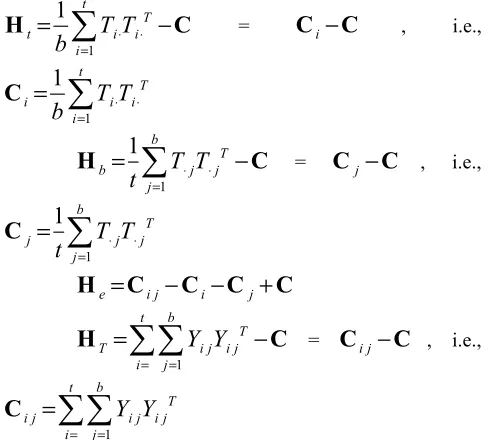
3.3. Calculations of Matrices of Sums of Squares (SS) and Cross-Products (SSCP)

Given the p-variate random vectors

N

X

~ 2 ~ 1

~

,

,...,

,

the total sum of squares can be partitioned as

1 T

T T b t

µ= ⋅⋅ ⋅⋅ =

(5)

1

t T

t i i

i

T T

b

₌ ⋅ ⋅

=

∑

−

H

C

=

C

_i

−

C

, i.e.,

1

t T

i i i

i

T T

b

₌ ⋅ ⋅

=

∑

C

1

b

T

b j j

j

T T

t

₌ ⋅ ⋅

=

∑

−

H

C

=

C

_j

−

C

, i.e.,

1

b

T

j j j

j

T T

t

₌ ⋅ ⋅

=

∑

C

e

=

i j

−

i

−

j

+

H

C

1

t b

T

T i j i j

i j

Y Y

= =

=

∑∑

−

H

C

=

C

_{i j}

−

C

, i.e.,

1

t b

T

i j i j i j

i j

Y Y

= =

=

∑∑

C

The dimension of each of the above matrices is

12 12

×

, where

T

_⋅⋅ is a 12-component vector of the sum of all the observations,

i

T

_⋅ is a 12-component vector of treatment total for each treatment,

j

T

_⋅ is a 12-component vector of block total for each block and

The equality of treatment effects is to be tested, i.e., In the multivariate model, we test for factor 1 (treatment) and factor 2 (block) as follows: Often, we wish to test the null hypothesis H0 : α1 = α2 = … = αa = 0 against the alternative H1: at least one αi≠ 0. These hypotheses specify no factor 1 effects and some factor 1 effect, respectively. We require the test statistic

(

)(

)

1

(

1

)

*

1 1 In

2

p a

a b

η= − − − − + − −  Λ

 

where

*

W

B W

Λ =

+

(2)

For a large sample, studies have shown that if

H

₀ is true then

η

approximately follows a chi-square

distribution with

p

(

k

−

1 )

degrees of freedom. At

α

level of significance,

H

₀ is rejected if

η χ

>

2_α

p k

(

−

1)

and accepted otherwise.

Using Bartlett’s correction, the likelihood ratio test is: Reject H0 : α1 = α2 = … = αa = 0 (no treatment effects) at level α if

2 ) ( p ) 1 a ( * ln 2

) 1 a ( 1 p ) 1 b )( 1 a

( _ ΛΛΛΛ >>>>χχχχ ₋₋₋₋ _αα_α_α

  



 ₋₋₋₋ ₋₋₋₋ ₋₋₋₋ ++++ −−−− −−−−

−−−− (3)

Where Λ* is given by equation (11) and

χ

₍2_a₋₁₎_p₍_α₎ is the upper (100α)th percentile of a chi-square distribution with (a – 1) df.

In a similar manner, factor 2 affects (block effect) are tested by considering H0 : β1 = β2 = … = βb = 0 and H1: at least one βj≠ 0. Small values of

res 1

fac res

SSCP

*

+

=

Λ

(4)

are consistent with H1. Again, for large samples and using Bartlett’s correction: Reject H0 : β1 = β2 = … = βb (no factor 2 effects) at level of α if

2 ) ( p ) 1 b (

*

ln

2 )

1 b

(

1 p

)

1 b

)(

1 a

(



Λ

>

χ

− α







+

−

(5)

Where Λ* is given by equation (13) and

χ

₍2_b₋₁₎_p₍_α₎ is the upper (100α)th percentile of a chi-square distribution with (b – 1)degree of freedom.

Manova Table for Comparing Factors

Source of variation

Matrix of sum of square and cross-products (SSCP)

Degrees of freedom

Block

H

_β a – 1

Treatment

H

_α b – 1

Residual (error)

H

_ε (a – 1)(b – 1)

Total (corrected for

the mean)

H

T Ab – 1

Note: This MANOVA table is consistent with the two-way MANOVA table for comparing factors and their interactions when n = 1. It is clear that when n = 1, SSCPres in the general two-way MANOVA table is a zero matrix with zero degrees of freedom. The matrix of interaction sum of squares and cross-products now becomes the residual sum of squares and cross-products matrix.

MANOVA can be used to investigate the dimensions on which groups differ. There are instances when an investigator wants to examine effects of independent variables across several dependent measures. MANOVA can be used to examine all of the DVs at the same time. Additionally, MANOVA controls Type 1 error (the probability of rejecting the null hypothesis when it is true) across all of the DVs in the model (Roberts, 2007).

Unlike conducting multiple ANOVAs, MANOVA accounts for the covariances of the other dependent variables, which might increase statistical power. That is, MANOVA has potential to be a more powerful test than univariate ANOVA because it considers both the variances and covariances of the dependent measures.

3.3.1. The Two-Way Anova Model

(6)

(Overall mean effect) ₍th_{treatment effect}_{) (}th_{block effect}_{) (}_{( , ) random effect}th ₎

i j i j i j

j

i i j

X = µ + α + β + ε

where

X

_{i j},

µ

,

α

_i,

β

_j and

ε

_{i j} are independent N(0, σ2)

random variables, and

0

_j

0

g 1 i i g 1 i

=

β

=

α

∑

= =

Motivated by the decomposition in equation (1), the analysis of variance is based upon an analogous decomposition of the observations,

(Observation) (Overall mean effect) ₍th

(

treatment effect

)

₎

(

₍th block effect

)

₎

(

(residual)

)

i j i j i j i j

j i

X = X⋅⋅ + X⋅−X⋅⋅ + X⋅ −X⋅⋅ + X −X⋅−X⋅ −X⋅⋅

) residual ( j i ij ) effect block estimated ( j ) effect treatment estimated ( i ) mean sample overall ( ) n observatio (

ij X.. (X. X..) (X. X..) (X X. X. X..)

X = + − + − + − − +

(6)

where

X

..

is an estimate of µ,

α

ˆ

i

=

(

X

i

.

−

X

..)

is an estimate of αi, and

β

ˆ

j

=

(

X

.

j

−

X

..)

is an estimate of βj, and

(

X

_ij

−

X

_i

.

−

X

.

_j

+

X

..)

is an estimate of the error eij.

Subtracting

X

..

from both sides of equation (6) and squaring produces + + − − + − + − = − 2 j i ij 2 j 2 i 2

ij X..) (X. X..) (X. X..) (X X. X. X..)

X ( + + − − − + −

−X..)(X. X..) 2(X. X..)(X X. X. X..) .

X (

2 _i _j _i _ij _i _j

..)

X

.

X

.

X

..)(

X

.

X

(

2

_j

−

_ij

−

_i

−

_j

+

(7)

Summing both sides of equation (7) over ij gives

+ − + − = −

∑

= = = = 2 j b 1 j 2 i a 1 i 2 ij b 1 j a 1 i ..) X . X ( a ..) X . X ( b ..) X X ( + − − = + − −

∑

= = = = ..) X . X ..)( X . X ( 2 ..) X . X . X X

( i j

b 1 j a 1 i 2 j i ij b 1 j a 1 i ..) X . X . X X ..)( X . X ( 2 ..) X . X . X X ..)( X . X (

2 j ij i j

b 1 j a 1 i j i ij i b 1 j a 1 i + − − − + + − − − ∑ ∑ ∑ ∑ = = = =

It is clear that sample algebra shows that the three cross products are zero. Therefore

2 j b 1 j 2 j a 1 i 2 i b 1 j a 1 i ..) X . X ( a ..) X . X ( b ..) X . X ( − =

∑

− +

∑

−

∑

= = = = 2 j i ij b 1 j a 1 i

..)

X

.

X

.

X

(

−

+

∑

= = (8)

represents a partition of the total sum of squares.

Expressing the Sum of Squares in equation (8) symbolically, we get

SSTotal = SSTreatments + SSBlocks + SSError (9)

The corresponding degrees of freedom associated with the Sums of Squares in the breakup in equation (8) are

ab – 1 = (a – 1) + (b – 1) + (a – 1)(b – 1) (10)

3.4. Multivariate Two-Way Fixed–Effect Model without Interaction

Proceeding by analogy, the two-way fixed-effects model for a vector response consisting of P components is

Xij = µ + αi + βj + eij (11) i = 1, 2, …, a

j = 1, 2, …, b

where

α

β

_j

0

g 1 i i g 1 i

=

∑

= =

the vectors are all of order p

x 1 and eij is assumed to be an Np(0, ε) random vector. Following equation (2), the observation vectors Xij can be decomposed as ..) X . X . X (X ..) X (X. ..) X . X ( .. X

Xij= + i − + j− + ij− i − j+ (12)

where

X

..

is the overall mean of the observation vectors,

.

X

i is the average of the observation vectors at the ith

level of treatment (factor),

X

.

_j is the average of the observation vectors at the jth level of block (factor 2). Thus, straightforward generation of equations (8) and (10) give the breakups of the sum of squares and cross-products and degrees of freedom:

++++ ′′′′ −−−− −−−− ==== ′′′′ −−−− −−−−

∑

==== ==== ==== ) .. X . X ..)( X . X ( b ) .. X X ..)( X X

( i i

a 1 i ij ij b 1 j a 1 i ) .. X . X . X X ..)( X . X . X X ( ) .. X . X ..)( X . X (

a ij i j ij i j

b 1 j a 1 i j j b 1 j ′′′′ ++++ −−−− −−−− ++++ −−−− −−−− ++++ ′′′′ −−−− −−−− ∑∑∑∑ ∑∑∑∑ ∑ ∑∑ ∑ ==== ====

==== (13)

ab – 1 = (a – 1) + (b – 1) + (a – 1)(b – 1) (14)

3.4.1. Simultaneous Confidence Intervals for Factor Effects

When the null hypothesis of equal treatment effects is rejected, it is necessary to determine the linear combination of parameters that caused this rejection. For a pairwise comparison, the Bonferroni method can be used to construct simultaneous confidence intervals. The choice of this approach is based on the fact that it provides shorter intervals than other methods (Niel, 1975). For any two treatments effects

t

_i and

t

_j , the

100 (

1 −

α

)

%

simultaneous confidence interval is given by Johnson(1982) as

(

)

1 1 1 1 ii

li ij _N

ii l j

W X X t

pk k n n n

α

−     − ± _ _ _ + _ −     Where ii

W

is the ith diagonal elements of

W

.

αii′–αmi′ belongs

to bn 2 v E ) 1 a ( pa t ) . X . X

( ii

v i m i i ′ ′ ′ ′       − α ±

− (15)

(7)

= SSCPres and

X

i

.

i′

−

X

m

.

i′ is the i′th component of

⋅

−

m

i

.

X

Similarly, the 100(1 – α)% simultaneous confidence intervals for βji′ – βqi′ are

βji′ – βqi′ belongs to

an 2 v E ) 1 a ( pa t ) . X . X

( ii

v i q i j

′ ′ ′

′ 

  

 

− α ±

− (16)

where v and Ei′i′ are defined above and

X

.

ji′

−

X

.

qi′ is the

ith component of

X

.

_j

−−−−

X

.

_q

4. Results and Discussion

In this section, the statistical method discussed in this paper has been employed to analyze financial ratio data of Nigeria from in. The mean vectors corresponding to the seven different vegetative covers are as follows. From the foregoing, it can deduced that the grand mean vector

66.00 34.61 27.50 44.54 4.55 1.11 41.20 2.84 2.87 2.55 27.80 16.74

67.75 38.27 27.00 48.81 27.85 1.06 48.14 1.44 21.45 2.56 23.56 25.27

69.00 37.79 25.50 44.47 54.78 1.14 38.92 1.05 19.62 2.61 24.43 17.92

69.00 35.82 26.50 41.82 58.92 1.13

=

X 36.30 1.13 1.86 2.55 24.57 16.27

68.50 37.24 25.50 44.10 30.79 1.11 40.22 1.27 9.63 2.56 25.08 20.21

68.00 35.82 26.50 41.82 58.92 1.13 36.30 1.13 1.86 2.55 24.57 16.27

69.50 38.13 24.50 42.80 56.71 1.09 38.92 1.15 7.86 2.53 23.56 19.56 

  



   

 

 _

The matrix of between treatment sum of squares and cross product is

45.357 24.874 -18.643 -24.248 652.126 0.008 -41.180 -11.778 35.742 -0.007 -30.429 5.644 24.874 46.189 -20.101 25.076 370.703 -0.484 42.698 -11.116 179.664 0.067 -36.336 62.220 -18.643 -20.101 24.857 23.207 -326.914 -0.122 39.582

B=

8.868 -20.553 -0.044 20.441 2.734 -24.248 25.076 23.207 115.328 -540.208 -0.942 187.466 5.688 300.379 0.240 -11.525 129.983 652.126 370.703 -326.914 -540.208 10783.06 1.534 -913.111 -204.286 170.456 0.205 -415.887 -145.807

0.008 -0.484 -0.122 -0.942 1.534 0.022 -2.063 -0.065 -1.465 0.012 0.134 -1.092 -41.18 42.698 39.582 187.466 -913.111 -2.063 328.349 13.364 412.946 -0.231 -12.442 204.673 -11.778 -11.116 8.868 5.688 -204.286 -0.065 13.364 6.286 -33.836 -0.101 15.814 -9.805

35.742 179.664 -20.553 300.379 170.456 -1.465 412.946 -33.836 1385.383 2.817 -146.287 456.864 -0.007 0.067 -0.044 0.240 0.205 0.012 -0.231 -0.101 2.817 0.017 -0.156 0.412 -30.429 -36.336 20.441 -11.525 -415.887 0.134 -12.442 15.814 -146.287 -0.156 53.915 -65.758

5.644 62.22 2.734 129.983 -145.807 -1.092 204.673 -9.805 456.864 0.412 -65.758 199.423

 

 

 

826.0061

B

=

Also, the within treatment sum of squares and cross product is

270.750 75.800 -123.000 -33.865 -70.832 -0.202 -73.165 -0.772 -0.208 -2.009 4.552 -41.063

75.800 232.817 -55.44 8.303 -129.382 0.115 -22.974 -3.269 2.847 0.205 -36.74 41.51

-123.000 -55.44 283.000 45.850 -3.380 -0.160 101.960 3.3

W=

20 0.055 -1.007 27.905 21.665

-33.865 8.303 45.85 115.375 2.871 0.206 59.035 5.24 -0.500 2.938 -1.966 119.725

-70.832 -129.382 -3.38 2.871 5541.888 0.553 -11.282 8.109 62.322 -0.776 11.095 4.221

-0.202 0.115 -0.16 0.206 0.553 0.027 -0.417 0.078 0.073 0.044 0.375 -0.167

-73.165 -22.974 101.96 59.035 -11.282 -0.417 148.638 2.791 -1.430 0.927 -2.459 62.959

-0.772 -3.269 3.320 5.240 8.109 0.078 2.791 1.194 0.555 0.302 3.046 2.459

-0.208 2.847 0.055 -0.500 62.322 0.073 -1.43 0.555 2.407 0.115 0.421 -1.061

-2.009 0.205 -1.007 2.938 -0.776 0.044 0.927 0.302 0.115 0.305 0.516 2.3765

4.552 -36.74 27.905 -1.966 11.095 0.375 -2.459 3.046 0.421 0.516 62.322 -63.879

-41.063 41.510 21.665 119.725 4.221 -0.167 62.959 2.459 -1.061 2.3765 -63.879 186.443

 

 

(8)

316.107 100.674 -141.643 -58.113 581.294 -0.194 -114.345 -12.550 35.534 -2.016 -25.877 -35.419 100.674 279.006 -75.541 33.379 241.321 -0.369 19.724 -14.385 182.511 0.272 -73.076 103.730 -141.643 -75.541 307.857 69.057 -330.2

B W+ =

94 -0.282 141.542 12.188 -20.498 -1.051 48.346 24.399 -58.113 33.379 69.057 230.703 -537.337 -0.736 246.501 10.928 299.879 3.178 -13.491 249.708 581.294 241.321 -330.294 -537.337 16324.95 2.087 -924.393 -196.177 232.778 -0.571 -404.792 -141.586 -0.194 -0.369 -0.282 -0.736 2.087 0.049 -2.480 0.0128 -1.392 0.056 0.509 -1.259 -114.345 19.724 141.542 246.501 -924.393 -2.48 476.987 16.155 411.516 0.696 -14.901 267.632

-12.550 -14.385 12.188 10.928 -196.177 0.0128 16.155 7.480 -33.281 0.201 18.860 -7.346 35.534 182.511 -20.498 299.879 232.778 -1.392 411.516 -33.281 1387.79 2.932 -145.866 455.803 -2.016 0.272 -1.051 3.178 -0.571 0.056 0.696 0.201 2.932 0.322 0.360 2.788 -25.877 -73.076 24.399 -13.491 -404.792 0.509 -14.901 18.86 -145.866 0.36 116.237 -129.637 -35.419 103.73 21.665 249.708 -141.586 -1.259 267.632 -7.346 455.803 2.788 -129.637 385.866

 

 

 

4.442451e+18

B W

+

=

5. Average Results of the Treatments

per Response Comments on the

Average Results

The matrix

X

shows the average results of the mechanical analysis. In the first three columns of the mean matrix, we observed that textural class of all the treatments was sandy clay loam. This in effect means that various vegetative covers have no effect on the textures of the soil.

The fifth and sixth columns of the mean matrix show the average results of the effects of various covers on the infiltration rate and the hydraulic conductivity of the soil, respectively. The highest and least rates of infiltration were observed on plots with bare fallow and creeping grass, respectively. The other covers namely, pueraria, “original”, stylosanthes, guinea and carpet had rates in-between these two extremes. This result could be explained by the fact that bare fallow plots were exposed to adverse effect of weather, thus resulting in crust formation on the soil surface, consequently hindering movement of water into the soil. Plots with covers on the other hand had higher rates of infiltration probably due to the fact that the grasses protect the soil against direct raindrops impact thereby preventing or minimizing the destruction of soil structure.

Hydraulic conductivity was highest on plots with carpet grass and least on plots under original grass. One would expect hydraulic conductivity to follow the same pattern as infiltration rate. This is because hydraulic conductivity is the readiness with which water flows through the soil in response to a given gradient. This disparity in trend was probably due to error of measurement. The rest of the columns of the mean matrix indicate the average results of some of the physical analysis, namely, total porosity, capillary porosity, air-space porosity, moisture content at field capacity, bulk density, particle density and penetrometer resistance of the soil.

From the mean matrix it could be observed that total porosity and moisture content at field capacity showed similar trends. Soils under “original” cover had the lowest total porosity and moisture content. On the other hand, soils under carpet covers had the highest total porosity and

moisture content. Soils under bare fallow ranked second for both variables. The variation in the results could be attributed to the rooting systems of the different covers.

Soils under bare fallow had the least air-space porosity and carpet cover the highest. Other vegetative covers ranked between these extreme in this order: “original” cover < guinea cover < peuraria < creeping cover < stylosanthes. This result could probably be due to the fact that their roots aided in aggregating soil particles into clods, thereby increasing the pore space between individual particles.

The average effect of different vegetative covers on penetrometer resistance is also indicated on mean matrix. This is an indicator of surface hardness or crust formation on the surface soil. It was observed that the greatest penetrometer reading was obtained under soils on bare fallow plots and the least on creeping cover. Other covers have figures between 2.53kg/m2 for soil under bare fallow and 1.05kg/m2 for creeping grass in the following order: carpet grass > stylosanthes > guinea grass > peuraria > “original” grass. These results indicated that vegetative cover has some loosening effect on the soil.

We shall examine the significance of these vegetative covers in what follows.

To obtain the determinant of this matrix we used R Software package in calculating the determinant of a matrix. Thus, the determinant is computed to be -1.641889E-23.

Now, under the null hypothesis that the variables are uncorrelated in the population from which they arose, we compute the value of the test statistic as follows:

V= –mloge |R|

=

log

(

0 .

019 )

6 )

5 )

12 (

2

335 (

e

+

−

= (–330.164)(–3.963) = 1308.451

6. Conclusion

(9)

method of analysis is henceforth adopted.

7. Analysis Using MANOVA

The matrices of the appropriate sum of squares and cross-products were calculated (see the SPSS statistical software output in Appendix I), leading to the following MANOVA table.

Source of variation

Degrees of freedom

value of

Λ ΛΛ Λ*

Matrix of sum of squares and cross-products (SSCP) Factor 1:

vegetative cover 6 0.000 Wα

Factor 2: Block 3 0.003 Wβ

Residual 18 We

Total 27 WT

To test for factor 1 (vegetative cover) and factor 2 (block) effects, we require

*

1.8593476889221738180117237083763e-16 B

B W

Λ = =

+

and

003 . 0 SSCP SSCP

SSCP *

res 2

fac res

2 = + =

Λ

for a – 1 = 6 and b – 1 = 3

[

]

[

|(a 1) p| 1

]

/2

2 / 1 p ) 1 b )( 1 a ( *

* 1 F

1 1 1

+ − −

+ − − −    

 

Λ Λ − =

and

[

]

[

|(b 1) p| 1

]

/2

2 / 1 p ) 1 b )( 1 a ( *

* 1 F

2 2

2 − − +

+ − − −

   

 

Λ Λ − =

Have F-distribution with degrees of freedom

V1 = |(a – 1) – P| + 1, V2 = (a – 1)(b – 1) – P + 1, respectively

Thus, F1 = 6.488, F2 = 3.511 (see appendix I) and v1 = |6 – 12| + 1 = 7, v2 = 18 – 12 + 1 = 7 From above, F7,7,0.05 = 3.79

We have F1 = 6.488 > F7,7,0.05 = 3.79, and therefore we reject H0 : α1 = α2 = … = α7 = 0 (no factor 1 effects) at the 5% level. Similarly, F2 = 3.511 < F7,7,0.05 = 3.79, and we do

not reject H0 :

β

ˆ

1

=

β

ˆ

2

=

β

ˆ

3

=

β

ˆ

4

=

0

(no factor 2 effects).

8. Conclusion

From the analysis of the data of this experiment, it is important to examine the various results at different stages. The highest mean for penetrometer resistance was obtained under bare fallow (2.53kg/m2). This is an indication that penetrometer resistance is inversely proportional to the present and abundance of cover as well as the type of cover on the soil. The highest infiltration rate was obtained under creeping grass (61.00cm/hr) and the least on bare fallow. Similar reports could be made for other responses.

The test for independence of the 12 responses shows that they are correlated in the population from which they arose, being acceptable as 5 percent significant level.

In the sequel, testing for the significance of treatment effects, we discovered that they are highly significant at 5 percent level of significance.

A close examination of the α-matrix that is, the matrix of the best linear unbiased estimates of the treatment effects shows that a good number of the treatments had negative effects on the responses. The most striking is the effect of the various treatments on penetrometer resistance where only bare fallow had positive effects.

From the test for significance of the treatment effects and the subsequent estimates of such effects, we would conclusively say that all the vegetative covers improved the measured physical conditions of the soil. The estimates under penetrometer resistance will be highly welcome since according to Ejiogu (1983), “positive values of penetrometer resistance in any soil are undesirable since soils with hard surface have positive value positive values for penetrometer resistance”.

Recommendation

In view of the fact that the scope of the analysis of this work is involving we restricted ourselves to testing only the significance of the treatment effects and finding their best linear unbiased estimates. Moreover, in view of the importance attached to this section of the work, we recommend that: the results of this work should be applied with care. In view of the above we suggest that a further study be carried in this field to consider some aspects of the work like multiple comparisons, as the technique is stated in this research work, which we did not undertake due to time and many constraints.

Appendix I

The layout of the design

Treatment:

Block

1 2 3 4

1 D B A G

2 A C B E

3 B E F B

4 F G E A

5 G D C D

6 E F D C

7 C A G F

Spss Computer Printout

General Linear Model Bartlett’s Test of Sphericitya

Likelihood ratio Approx. Chi-Square df

Sig.

.000 680.771

(10)

Tests the null hypothesis that the residual covariance matrix is proportional to an identity matrix.

a. Design: Intercept + Treatment + Block

Multivariate Testsc

Effect Value F Hypothesis df Error df Sig. Partial Eta Squared

Intercept

Pillai’s Trace Wilks’ Lambda Hotelling’s

Trace Roy’s Largest Root

1.00 .000 24258.607 24258.607

14150.854a 14150.854a 14150.854a 14150.854a

12.000 12.000 12.000 12.000

7.000 7.000 7.000 7.000

.000 .000 .000 .000

1.000 1.000 1.000 1.000

Treatment

3.613 .000 2995.175 2974.816

1.514 6.488 221.865 2974.816b

72.000 72.000 72.000 72.000

72.000 43.889 32.000 12.000

.040 .000 .000 .000

.602 .892 .998 1.000

Block

2.491 .003 19.808 11.420

3.674 3.511 3.118 8.565b

36.000 36.000 36.000 12.000

27.000 21.410 17.000 9.000

.000 .002 .007 .002

.830 .851 .868 .919

Appendix II

Data for total porosity

Treatment:

Block

1 2 3 4

Bare 43.97 43.10 45.10 45.97

Carpet 47.97 46.50 50.08 51.16

Creeping 42.30 42.00 46.64 46.94

Guinea 42.55 45.46 45.79 42.55

Original 38.85 38.87 44.76 44.78

Stylosanthes 40.92 45.50 48.50 43.92

Pueraria 42.50 43.00 43.10 42.60

Data for intiltration rate

Treatment:

Block

1 2 3 4

Bare 4.11 5.34 5.00 3.75

Carpet 14.49 41.21 42.36 13.35

Creeping 74.22 28.57 35.34 81.00

Guinea 20.76 42.81 18.78 40.83

Original 69.37 48.47 18.78 40.83

Stylosanthes 21.39 24.52 15.62 12.49

Pueraria 68.01 84.80 45.41 28.63

Data for bulk density

Treatment:

Block

1 2 3 4

Bare 1.12 1.13 1.05 1.14

Carpet 0.98 1.07 1.06 1.12

Creeping 1.10 1.13 1.16 1.16

Guinea 1.08 1.11 1.12 1.12

Original 1.13 1.12 1.17 1.09

Stylosanthes 1.17 1.17 1.09 1.15

Pueraria 1.08 1.09 1.12 1.08

Data for moisture content of the soil

Treatment:

Block

1 2 3 4

Bare 39.45 39.04 42.94 43.35

Carpet 48.87 48.65 47.40 47.62

Creeping 37.68 36.67 40.12 41.19

Guinea 39.41 37.27 40.99 43.19

Original 34.32 35.62 38.28 36.98

Stylosanthes 34.98 35.01 44.64 44.36

Pueraria 39.29 39.27 38.57 38.53

Data for penetrometer resistance

Treatment:

Block

1 2 3 4

Bare 2.81 2.41 2.29 2.61

Carpet 1.01 1.80 1.41 1.55

Creeping 0.83 0.74 1.39 1.24

Guinea 1.38 1.12 1.36 1.22

Original 0.94 0.89 1.21 1.47

Stylosanthes 1.16 1.34 1.25 1.35

Pueraria 0.87 1.37 1.19 1.16

Data for hydraulic conductivity

Treatment:

Block

1 2 3 4

Bare 2.90 2.88 2.89 2.79

Carpet 20.59 22.18 21.39 21.65

Creeping 20.27 18.98 19.60 19.63

Guinea 9.41 9.83 9.62 9.67

Original 1.78 1.95 1.87 1.85

Stylosanthes 12.45 12.31 12.22 12.21

(11)

Data for particle density

Treatment:

Block

1 2 3 4

Bare 2.50 2.64 2.42 2.64

Carpet 2.35 2.60 2.63 2.65

Creeping 2.45 2.65 2.68 2.67

Guinea 2.38 2.67 2.57 2.63

Original 2.35 2.58 2.62 2.66

Stylosanthes 2.48 2.66 2.61 2.61

Pueraria 2.38 2.64 2.47 2.64

Data for capillary porosity

Treatment:

Block

1 2 3 4

Bare 30.94 25.15 23.17 31.94

Carpet 23.14 24.25 22.75 24.09

Creeping 24.98 24.68 23.63 25.43

Guinea 26.33 24.98 23.68 25.31

Original 24.50 24.51 24.62 24.63

Stylosanthes 23.50 23.93 23.66 23.62

Pueraria 22.93 23.93 23.71 23.68

Data for air-space porosity

Treatment:

Block

1 2 3 4

Bare 13.03 17.95 21.93 14.03

Carpet 24.34 22.25 27.43 27.07

Creeping 17.32 17.32 23.01 22.51

Guinea 16.22 20.31 21.81 17.24

Original 14.35 13.36 20.14 20.21

Stylosanthes 17.42 21.57 24.84 20.40

Pueraria 19.57 19.07 19.39 18.92

References

[1] Adeoye, K.B. (1982): Effect of tillage depth on physical properties of a tropical soil and on yield of maize sorghum and cotton. Soil Tillage Research, 2; 225 – 231.

[2] Egwuatu, U.T. (1982): The Effects of Different Ground Cover on the Physical Properties of Nkpologu Series. [3] Enyioku, C.O.; Obi, M.E. and Eneje, R.C. (2012): Soil

Water Characteristics and Structural Stability of a Typic Paleustult under different Vegetation Cover. Publication of

Nasarawa State University, Keffi,

www.patnsukjournal.net/currentissue

[4] Lal R., (1998): Methods for assessment of soil degradation. In: Advances in Soil Sciene. CRP Press, Boca Raton fl. [5] Lugo, Lopez, M.A.; Wolf, J.M. and Perez Escolar, R. (1981):

Water loss, intake movement retention and availability in major soils of Puerto Rico. University of Puerto Rico Bulletin 264. pp. 7 – 8.

[6] Mbagwu, J.S.C. and Ekwealor, G.C. (1990): Agronomic potential of brewer’s spent grain. Biological Wastes, 34:335 – 347.

[7] Mbagwu, J.S.C. (1989): Effect of organic amendments on some physical properties of a tropical ultisol. Biological Wastes 28: 1 – 13.

[8] Montgomery, D.C. (1976): Design and Analysis of Experiment. New York, John Willey and Sons.

[9] Obi, M.E. (1982): Runoff and soil from an oxisol in southeastern Nigeria under various management practices, Agric water manage, 5:193 – 203.

[10] O’Brien, R. G. & Kaiser, Mary Kister (1985). MANOVA method for analyzing repeated measures designs: An extensive primer. Psychological Bulletin, 97, 316-333. [11] Papendick, R.I. and Campbell, G.S. (1981): Theory and

measurement of water potential. In: J.F. parr, W.R., Gardner, and L.F. Elliot (eds. Water Potential Relations in soil Microbiology, Special publication no. 9 Soil Science Soc amer, Madison Wiscoson pp. 1 – 22.

[12] Richard, A.J. and Dean, W.W. (1992): Applied Multivariate Statistical Analysis. Prentice Hall, Englewood Cliffs, New Jersey.

[13] Spaan, W.P.; Silking, A.F.S. and Hoogmoed, W.B. (2005): Vegetation barrier and tillage effects on runoff and sediment in an alley crop system on Luvisol in Burkina Faso. Soil and Tillage Research, 83: 194 – 203.

[14] Tollner, E.W.; Hargrove, W.L. and Laongdale, G. (1984): Influence of conventional and no-till practices soil physical properties in the southern Piedmont. Journal of soil and water conservation. 39:72 – 76.