Layering of CDMA Wireless Sensor Network Cluster to Improve Network Capacity

Vol.9 (2019) No. 4

ISSN: 2088-5334

Layering of CDMA Wireless Sensor Network Cluster to Improve

Network Capacity

Dwi Widodo Heru Kurniawan

, Adit Kurniawan

, M Sigit Arifianto

STEI, Institut of Technology Bandung, Ganesha Street, Bandung, 40132, Indonesia E-mail:[email protected]; [email protected]; [email protected]

Abstract—Nowadays, the network capacity of the wireless sensor network is a critical research topic area in the world. As the number

of sensors connected to the network is quickly growing, it is important that they can sense and transmit data instantly. One of the approaches to increase the network capacity is clustering the sensors to control communication. The approach will divide sensors into several groups and drive the sensors to send the data through the cluster head. However, the approach will arise inter-cluster interference problems from the sensors near the border that is higher level than other sensors. All of those will cause the fewer sensor that can send the data so that reducing the network capacity. In order to overcome the problem, layering the sensor cluster is proposed which each cluster is divided into two layers. Moreover, the outer layer is divided into four zones and assigned one intermediary sensor in each zone. Sensors in the outer layer will communicate with the cluster head through the intermediary sensors. The method will reduce the transmission power and lessen the interference to other clusters. The approach not only can minimize interference coming from the sensors near the outer layer but also reduce the power consumption. The study concludes that applying the layering technique will drive the sensors near the border to generate minimum interference in their cluster and neighbor clusters. As a result, the network can deliver more capacity than approaches using either only clustering or layering.

Keywords— network capacity; cluster; layering; interference.

I. INTRODUCTION

Sensors provide intelligence for smart cities by providing useful information to enhance people’s life. These sensors sense, collect, and transmit data into the sink [1]. The data is then processed into useful information for monitoring and controlling the city's situation and directing people's movement efficiently. The sensors autonomously build a wireless sensor network (WSN) and collaborate to collect data [2]. As the number of sensors connected to the network is growing, network capacity is becoming an important issue. As with other wireless communications, the network capacity of code division multiple access (CDMA) wireless sensor networks is affected by the quality of the signal (Eb/I0)

which determines the bit error rate (BER) in the destination sensor [3][4]. One of the factors that impact directly on the BER of signals is the strength of interference. Higher interference means many errors occur in the network, and fewer sensors can transmit data in parallel.

Many efforts to overcome this problem have been completed by controlling the communication inside the network. The network is partitioned into several sub-networks to reduce complexity, and the sensors are divided into clusters that group sensors based on the deployment or power transmission [5]. In this paper, the author layers the

clusters into two-layer and studies interference in the network. With this approach, the network capacity will be improved with the preservation of energy consumption at a minimum level [6].

Research on wireless sensor networks focuses on reducing interference and improving the lives of the network by maintaining low energy consumption. Reference [6] studied the cross-layer implementation in the network layer, medium access control (MAC) layer, and the physical layer to increase the network existence. The optimization problem encompasses routing, link scheduling, rate of transmission, and power distribution. Using the approach, varying source rate, link scheduling, and node’s placement can maximize the network lifetime. Reference [7] proposes two novel advances to achieve accuracy and approximation estimation of signal to interference and noise ratio (SINR) distribution in a wireless sensor network. This SINR distribution can be used to evaluate the throughput or the WNS’s capacity.

threshold, the paper concludes that there is an optimum number that maximizes the outage capacity. Reference [9] evaluates the relationship between interference and traffic. The research shows that increasing the traffic will generate higher interference and collision in the receiver node. Then, the sender node spends more energy to retransmit the data. The research proposes a new method to overcome the problem by creating a new route of data transmission using a low loaded neighbor node.

Several works address optimum number of the router used in WSN to reduce interference but still maintain the system reliability [10], find a spanning tree that minimize the receiver’s interference by using RIP and MinMax-BRIP algorithm [11], and derive transmitted power that consider relationship between interference and network activity by using stochastic geometry theory [12]. In the current work, we analyze the interference’s effect from the sensors near the border in the layering wireless sensor cluster and the effect on energy depletion and the capacity of the network. The paper is composed of three sections. Section I is the introduction of the research and the related work. Section II introduces the material and method (include network capacity and energy analysis); Section III shows the results and discussion.

II. MATERIALS AND METHOD

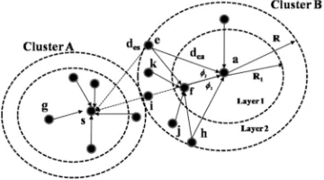
Sensors near the border generate an interference power higher than other sensors. To overcome this, the author proposes layering the cluster of the wireless sensor network cluster (Fig. 1). Each cluster was divided into two layers, layer one and layer two. A sensor in layer two will transmit the data into the cluster head (CH) through an intermediary node in layer one. There are two types of interference generated by sensors cluster B in layer 2. They interfere with other clusters around cluster B (inter-cluster interference) and interfere with its cluster (intra-cluster interference). With layering, the transmission power of the sensors in layer two will decrease and generate less interference. To evaluate the impact of interference, the author uses the network model in Fig. 1, with the performance indicator being average interference per cluster, network capacity, and average energy per cluster. Then the author compares this model with two other models, namely the cluster network and layering network.

Fig. 1 Layering of the wireless sensor network cluster

The network model uses a random uniform distribution for sensor deployment. Let m be a signal path loss exponent, and then sensor e generates inter-cluster interference in CHs:

, _∅ / , (1)

If t=zas/zea and p=R1/R then (1) becomes:

∅ /

∅ / (2)

where t is the ratio of the distance between the cluster head (example zas) and the distance between the sensor and its

cluster head (example zea). Sensor e generates intra-cluster

interference in CHa:

_, ∅

/

/ , (3)

Following [3], the interference signal follows the probability distribution function (pdf):

!"

⎩ ⎪ ⎨ ⎪

⎧"'!" () !* '

+'!"( ()

,!_* " + - +

, ./ !* +

" 1 1

!* -"

!_{* - +}

, _{" +} , ./

!*

-" 1 1

(4)

where:

Pr is the receiving power

PI is the interference power

z0 is the smallest range between sensors

zR is the highest sensor range

zI is the interfering sensor range

m is the signal path loss exponent.

The amount of interference power from sensors near the border can be represented by the average value of the interference power with distribution following (4). The average interference between clusters is calculated:

(5)

The lower bound and the upper bound of (5) is

0 1 1 _∅∅ // , (6)

Applying the bound in (6) with probability distribution function following (4), then the average interference signal power E[PI] is as follows:

(7)

where:

The sensor f controls the transmission’s power of the sensor e and the interference to CHa. Implementing the

same method as (7) resulting in (PI)e,a:

(8)



∞

∞ −

= I I I

I P f P dP

P

E[ ] ( )





I d P

E DP P p d C BP AP P P E ) 414 . 1 2 1 ( ) 414 . 1 2 1 ( Pr 2 1 1 2 2 1 0 1 2 1 2 ) ( ) ( ] [ ) ( ); ( ) )( ( ; ; 2 0 2 2 0 2 2 2 0 2 2 0 2 2 4 0 4 4 d d m E d d P D d d d d mP C d P B d A I R m r R I m r m r I − = + = − − = = =

(

)

m a

e

I p p P

P ,

2 / 2

, 1 1.414

)

For Ø2=00, the interference from sensor i to cluster A is:

(9)

The sensor’s position influences the amount of interference of the sensor into the cluster head. Sensor i has high interference into CHs compare to other sensors as its

position is nearest to CHs. However, sensor i generates the

lowest interference to CHa because its position is nearest to

intermediary sensor f, and it needs low transmission power to send data into CHa. The p variable has a value between

zero and one when the layer moves from the centre into the cluster’s border. If the layer is near the cluster head, the sensors are mainly located in layer two and produce excessive inter-cluster interference but little interference with its cluster. The contrasting case takes place when p moves to 1. Most of the sensors are located in the inner layer, and fewer sensors are located in the outer layer. The p variable has a minimum impact at the position between the centre and the border of the cluster.

A. Network Capacity Analysis

Network capacity is an indicator to measure how many sensors can send data simultaneously. In the CDMA environment, the successful delivery of data is determined by the Eb/I0 signal received in the destination sensor. A

lower Eb/I0 means a higher bit error rate. The interference

inside the cluster and from other clusters will affect the number of sensors that can be active at one time. A particular cluster capacity depends on another cluster capacity [13]. Increasing the capacity of one cluster will decrease another cluster capacity. If the capacity is growing, then it produces more signal and high interference to other clusters. Because the interference in a cluster is limited to the threshold value, the cluster will decrease active sensors to keep the performance above a certain threshold.

(10)

Equation (10) shows the relationship between the threshold value ceff and the sum of interference in a cluster.

The interference should be lower than the threshold to keep the performance excellent. Several factors influence the threshold like the processing gain, the number of active sensors (α), and Eb/N0. The equation (10) is the network

capacity linear programming. Applying (10) into the network model (Fig.1) will solve the optimization problems for CDMA wireless sensor network. The objective is to find maximum sensors in every cluster with the total interference is lower than the threshold value. The total interference is computed from the average interference power and the number of sensors in each cluster.

Objective function: (11)

Constraint: (12)

where: n is sum of the sensors in a cluster M is sum of the clusters

κ is the interference factor W is the bandwidth of a signal T is Eb/I0 threshold

I is the average interference power metrics X is sum of the sensors in every cluster metric ceff is the maximum of active sensors in a network

B. Energy Analysis

Sensors use energy to sense the data and then transmit it into the cluster head, while the sensor that acts as a cluster head does several activities as other sensors and an additional job like receiving data from sensor member, aggregating and transmitting it into the sink. The energy consumption in a sensor will increase when it becomes a cluster head. Energy consumption in CDMA wireless sensor networks is affected by the transmission power, the number of bits transferred, and the number of retransmissions.

(13)

where: Ea is energy consumption

α is the activity factor Pt is the transmission power

Lb is sum of bits transferred

Rb is the transmission rate

K is the number of retransmission (due to error).

Variable K shows how many retransmissions occur caused by the error, and depends on the average PER (packet error rate) [14].

(14)

If one packet consists of Lb bits, then the probability of

packet error depends on the probability of bit error (pe):

(15)

The distance between sensors and the received power in the receiving sensor influences energy spending in the network. In CDMA, the receiving signal will be kept constant by power control. The average energy consumption depends on the random variable distance.

(16)

If y=dm with the probability distribution function (pdf) following [3], we can then calculate average energy consumption.

(17)

Evaluating average energy consumption by equation (16) using pdf in equation (17), we obtain:

(18)

(

)

m a

i

I p p P

P ,

2 / 2

, 1 2

) ( = + − b b t a R KL P E =α

) 1 ( 1 PER K − = b L e p PER=1−(1− )

b b r m R KL P d E=α

(

)

f m m

m Y , 0 , , ) ( 2 )

( 2 0

0 2 1 2 ) 1 ( ] [ PER R L R KL E E b b b b a − =

=α α

eff b M j ji j i c N E T R W n

n _+ ≅

III.RESULTS AND DISCUSSION

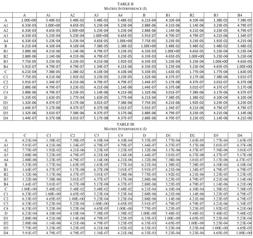
To analyze the effect of the layering model on the CDMA wireless sensor network cluster, we apply (7), (11), (12), and (18) with the parameters in Table 1. The interference matrix to solve optimization is using Table 2 and Table 3, with the performance indicators evaluated, namely average interference, network capacity, and energy consumption with the network model shown in Fig. 1.

TABLEI

NETWORK PARAMETERS

Variables Numbers Unit

Pr -70 dBm

zR 25 Meter

zI 56 Meter

W/R 20 dB

T 9.2 dB

m 4

Lb 1,064 Bits

Rb 20 Kbps

α _0.375

For the evaluation, the author sets up 4 clusters, and each cluster has two layers. To serve the sensors in the outer layer, the author defines four zones and allocate one intermediary sensor for each zone, presented in Fig.2.

Fig. 2 Layering wireless sensor network cluster

TABLEII MATRIX INTERFERENCE (I)

A A1 A2 A3 A4 B B1 B2 B3 B4

A 1.00E+00 5.48E-02 5.48E-02 5.48E-02 5.48E-02 6.21E-04 4.10E-04 4.10E-04 1.38E-02 7.38E-05 A1 6.33E-03 1.00E+00 4.65E-05 5.23E-04 5.23E-04 2.88E-06 4.21E-06 1.14E-06 3.23E-05 4.79E-07 A2 6.33E-03 4.65E-05 1.00E+00 5.23E-04 5.23E-04 2.88E-06 1.14E-06 4.21E-06 3.23E-05 4.79E-07 A3 6.33E-03 5.23E-04 5.23E-04 1.00E+00 4.65E-05 5.91E-07 4.79E-07 4.79E-07 4.21E-06 1.34E-07 A4 6.33E-03 5.23E-04 5.23E-04 4.65E-05 1.00E+00 7.75E-05 3.23E-05 3.23E-05 1.92E-02 4.21E-06 B 6.21E-04 4.10E-04 4.10E-04 7.38E-05 1.38E-02 1.00E+00 5.48E-02 5.48E-02 5.48E-02 5.48E-02 B1 2.88E-06 4.21E-06 1.14E-06 4.79E-07 3.23E-05 6.33E-03 1.00E+00 4.65E-05 5.23E-04 5.23E-04 B2 2.88E-06 1.14E-06 4.21E-06 4.79E-07 3.23E-05 6.33E-03 4.65E-05 1.00E+00 5.23E-04 5.23E-04 B3 7.75E-05 3.23E-05 3.23E-05 4.21E-06 1.92E-02 6.33E-03 5.23E-04 5.23E-04 1.00E+00 4.65E-05 B4 5.91E-07 4.79E-07 4.79E-07 1.34E-07 4.21E-06 6.33E-03 5.23E-04 5.23E-04 4.65E-05 1.00E+00 C 6.21E-04 7.38E-05 1.38E-02 4.10E-04 4.10E-04 5.33E-05 1.63E-05 1.77E-04 1.77E-04 1.63E-05 C1 7.75E-05 4.21E-06 1.92E-02 3.23E-05 3.23E-05 1.32E-06 4.37E-07 3.17E-06 7.38E-06 3.01E-07 C2 5.91E-07 1.34E-07 4.21E-06 4.79E-07 4.79E-07 1.44E-07 5.17E-08 4.37E-07 3.01E-07 6.37E-08 C3 2.88E-06 4.79E-07 3.23E-05 4.21E-06 1.14E-06 1.44E-07 6.37E-08 3.01E-07 4.37E-07 5.17E-08 C4 2.88E-06 4.79E-07 3.23E-05 1.14E-06 4.21E-06 1.32E-06 3.01E-07 7.38E-06 3.17E-06 4.37E-07 D 5.33E-05 1.63E-05 1.77E-04 1.63E-05 1.77E-04 6.21E-04 7.38E-05 1.38E-02 4.10E-04 4.10E-04 D1 1.32E-06 4.37E-07 3.17E-06 3.01E-07 7.38E-06 7.75E-05 4.21E-06 1.92E-02 3.23E-05 3.23E-05 D2 1.44E-07 5.17E-08 4.37E-07 6.37E-08 3.01E-07 5.91E-07 1.34E-07 4.21E-06 4.79E-07 4.79E-07 D3 1.32E-06 3.01E-07 7.38E-06 4.37E-07 3.17E-06 2.88E-06 4.79E-07 3.23E-05 4.21E-06 1.14E-06 D4 1.44E-07 6.37E-08 3.01E-07 5.17E-08 4.37E-07 2.88E-06 4.79E-07 3.23E-05 1.14E-06 4.21E-06

TABLEIII MATRIX INTERFERENCE (I)

C C1 C2 C3 C4 D D1 D2 D3 D4

Table 2 and Table 3 are the interference matrix that is evaluated using (7). Every cell shows an average interference factor between clusters, the farther distance between clusters is getting smaller the interference factors. First, the author evaluates the effect of layering ratio into interference and network capacity. The layering ratio determines the sensor’s distance in the outer layer from the intermediary sensor and influences the amount of interference for its cluster and other clusters. Fig. 3 plots the effect of the layering ratio on interference and network capacity. The percentage (%) indicator of interference power in Fig. 3 measures how much interference occurs in the cluster compared with its receiving power (-70 dBm).

The result shows that there is a little variation in interference power for layering ratio (p) between 0.1 until 0.5, which it decreases to minimum interference power at radius 0.7, then rises again. At layering ratio 0.7, the amount of interference power is only 6%, much lower than 24% (the highest contribution) at layering ratio of 0.1. This behavior occurs because of the distance variation between the sensors in layer 2 and the intermediary sensor. Besides interference, Fig. 3 shows network capacity in the network model. If interference is low, then the number of active sensors will increase, and vice versa. At point 0.7, the network will have a maximum capacity as it has the lowest level of interference.

Fig. 3 Effect of layer ratio on network capacity and interference

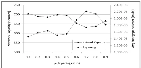
Second, the author evaluates the relationship between layering ratio and energy per cluster. Fig. 4 shows the effect of the layering technique on energy consumption. Same with interference, energy consumption tends to decrease from point 0.1 to 0.5, it decreases sharply to its minimum level at layering radius 0.7, then increasing again. At layering ratio 0.7, the amount of average energy per cluster 1x10-6 Joule compares to 2.2x10-6 Joule (2.2 times) at 0.1. The average energy consumption depends on the average packet error rate (PER), and the PER relies on the amount of interference taking place in the network. Higher interference will cause many transmission errors and the need for retransmission, and it increases energy consumption. That is why energy consumption shows similar behavior to the interference graph in Fig. 3.

Fig. 4 Effect of layer ratio on network capacity and average energy per sensor

Third, the author evaluates how the layering approach in CDMA wireless sensor network clusters could add network capacity. The simulation using the configuration in Fig. 2 results in a network capacity of 712 sensors with the sensor distribution is displayed in Fig. 5. Zone A, B, C, and D have the fewest number of sensors, while zone A1, A3, B1, B4, C2, C3, D2, and D4 own the largest sensors. The sensor distribution follows the interference pattern where the inner layer experiences interference from 4 zones and other clusters, whereas the outer layer only has little interference from the outer layer or the inner layer.

Fig. 5 Layering wireless sensor network cluster

The author simulates to increase the number of clusters, evaluate interference distribution and the growth of network capacity. Also, energy spending in the network is assessed. Fig. 6 presents the relationship between the number of clusters, network capacity, and average energy spending in the system.

On average, increasing the number of clusters by 76% will increase network capacity by nearly 27%, and also increases energy consumption by 2%. The study also shows that the growth in average energy consumption is almost the same as network capacity. Next, we compare the performance of layering in the cluster network (cluster layering) with the layering and cluster only approaches. In the layering approach, the network will be partitioned into several layers with the sink as the center, as shown in Fig.7. The method minimizes interferences by selecting a sensor in layer one to serve the outer sensor when it wants to send the data into the sink. For instance, if sensor h sends data to sensor e through intermediary sensor g and f. With this approach, the transmit power of sensor h will be reduced.

Fig. 7 Network model with a layering approach

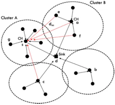
Another approach is network cluster, displayed in Fig.8. It applies network clustering to reduce interference where the cluster’s members send data through the cluster head. Then the cluster head will proceed with the data aggregation that combines data from several sensors and sends it into the sink. In this model, the transmission power of sensors will be controlled by the cluster head, and interference power depends on the distance between the sensors and cluster head.

Fig. 8 Network model with a clustering approach

Fig. 9 displays the impact of the three approaches on average energy consumption. The results show that energy consumption in the cluster layering approach is much lesser

than the other methods, then follows by layering and cluster. This means that the approach is more efficient than the other technique. Increasing the number of clusters shows little variation in energy consumption in the three methods.

Fig. 9 Number of cluster vs average energy per sensor

Fig. 10 shows the relationship between the number of clusters and network capacity (number of sensors). Increasing the number of clusters will increase network capacity. The study indicates that cluster layering delivers higher network capacity compares to the other approaches. Cluster layer's capacity is about 1.5 times that of the layering and about 6 times that of the cluster approach. Even though cluster layering results in higher capacity, the network capacity's growth is similar to the other methods (49%-52%). The reason for higher capacity is cluster layering result in four times new zone to cluster approach. Fig. 10 displays another interesting result that the curve of cluster layering and layering the only approach follow an exponential line, however, the cluster approach curve is linear.

Fig. 10 Number of clusters versus network capacity

IV.CONCLUSIONS

experiences higher interference than the outer layer will have the lowest network capacity. Vice versa, the outer most layer has lower interference than other layers, and it has the highest network capacity. The research shows that layering in CDMA wireless sensor networks is a superior approach to that of layering or clustering only methods. Network capacity will increase by 1.5-6 times if the layering cluster approach is applied.

REFERENCES

[1] Z. H. Mir and Y.-B. Ko, “Collaborative topology control for many-to-one communications in wireless sensor networks,” IEEE Access, vol. 5, pp. 15927–15941, 2017.

[2] S. Dong and C. Li, “The improvement of LEACH algorithm in wireless sensor networks,” Int. J. Online Eng., vol. 12, no. 11, pp. 46–51, 2016.

[3] D. W. H. Kurniawan, A. Kurniawan, and M. S. Arifianto, “An analysis of optimal capacity in cluster of CDMA wireless sensor network,” in Proceedings - 2017 International Conference on

Applied Computer and Communication Technologies, ComCom 2017,

2017, vol. 2017-Janua, pp. 1–6.

[4] B. & B. Nithya, V., Ramachandran, “ BER Eval. IEEE 802.15.4 Compliant Wirel. Sens. Networks Under Var. Fading Channels,",

Wireless Personal Communications, vol. 77, no. 4, pp. 3105–3124,

2014.

[5] S. K. Singh, P. Kumar, and J. P. Singh, “A survey on successors of LEACH protocol,” IEEE Access, vol. 5, pp. 4298–4328, 2017. [6] H. Yetgin, K. Cheung, M. El-Hajjar, and L. Hanzo, "Cross-Layer

Network Lifetime Maximization in Interference-Limited WSNs,",

IEEE Transactions on Vehicular Technology, vol. 64. 2015.

[7] M. Haraty, A. Mohammadi, and M. Mehbodnia, “Estimation of SINR distribution function in clustered wireless sensor networks using statistical distribution modeling,” in 7’th International

Symposium on Telecommunications (IST’2014), 2014, pp. 740–745.

[8] R. E. Rezagah and A. Mohammadi, “Outage threshold extraction for maximising the capacity of wireless ad hoc networks,” IET Commun., vol. 5, no. 6, pp. 811–818, 2011.

[9] M. Fereydooni and M. Sabaei, “An optimized model for interference and traffic aware topology control in WSNs,” in 2012 35th

International Conference on Telecommunications and Signal Processing (TSP), 2012, pp. 22–26.

[10] A. Ghosh, M. Lata, G. Konar, and N. Chakraborty, “Optimised use of nodes in Wireless Sensor Network: A novel approach to overcome the effect of interference,” in 2016 2nd International Conference on

Control, Instrumentation, Energy & Communication (CIEC), 2016,

pp. 506–510.

[11] D. P. Shetty and M. P. Lakshmi, “Algorithms for minimizing the receiver interference in a wireless sensor network,” in 2016 IEEE

Distributed Computing, VLSI, Electrical Circuits and Robotics (DISCOVER), 2016, pp. 113–118.

[12] J. Chen and B. Q. Kan, “Optimal link control of WSN considering the network activity interference with stochastic geometry theory,” in

2016 10th IEEE International Conference on Anti-counterfeiting, Security, and Identification (ASID), 2016, pp. 117–121.

[13] M. Khabbazian, S. Durocher, A. Haghnegahdar, and F. Kuhn, “Bounding interference in wireless ad hoc networks with nodes in random position,” IEEE/ACM Trans. Netw., vol. 23, no. 4, pp. 1078– 1091, 2015.

[14] U. Datta and S. Kundu, “Energy level performance of multi hop CDMA wireless sensor network with error control,” in 2012 IEEE