COMPARATIVE ANALYSIS OF TWO
MATHEMATICAL MODELS FOR PREDICTION OF
COMPRESSIVE STRENGTH OF SANDCRETE
BLOCKS USING ALLUVIAL DEPOSIT
B.O. Mamaa,b, N.N. Osadebea
a
Department of Civil Engineering, University of Nigeria, Nsukka, Nigeria
bEmail: [email protected]
Abstract
A mathematical modeling for prediction of compressive strength of sandcrete blocks was performed using statistical analysis for the sandcrete block data ob-tained from experimental work done in this study. The models used are Scheffes and Osadebes optimization theories to predict the compressive strength of sand-crete blocks using alluvial deposit. The results of predictions were comparatively analysed using the statistical package for social sciences (spss) for the students t-test.It was found that the two models are acceptable for the prediction of com-pressive strength of sandcrete blocks.
Keywords: sandcrete block, compressive strength, laterite, Scheffe’s theory, Osadebe’s theory
1. Introduction
In engineering field, sandcrete block is con-sidered to be similar to concrete block and is expected to exhibit properties similar to those of concrete except perhaps for its lower strength.
Concrete is a versatile construction mate-rial owing to the benefits it provides in term of strength,durability,availability,adoptability and economy. Great efforts have been made to improve the quality of concrete by various means in order to raise and maximize its level of performance.
Prediction of concrete strength has been active area of research and a considerable number of studies have been carried out. A number of improved prediction techniques have been proposed by including empirical or computational modeling and statistical tech-niques.
1.1. Computational modeling
Many attempts have been made for model-ing this process through the use of computa-tional techniques such as finite element anal-ysis but the computational complexity of the models is prohibiting in many cases, requiring non proprietary mathematical tools.
1.2. Statistical techniques
A number of research efforts have concen-trated on using multivariable regression mod-els to improve the accuracy of predictions.
interval for predictions. For these reasons sta-tistical analysis was chosen to be technique for strength prediction of this study.
Modeling the prediction of compressive strength of concrete: The most popular re-gression equation used in the prediction of compressive strength is:
F =bo+b1w/c (1)
Where F = compressive strength of concrete,
w/c = water/cement ratio and bo, b1 =
coef-ficients.
The earlier equation is the linear regres-sion equation. The origin of the equation is Abram’s law [1] which relates compres-sive strength of concrete to the w/c ratio of the mix and according to this law,increasing
w/c ratio will definitely lead to decrease in concrete strength. The original formular for Abram is:
F = A
Bw/c (2)
Where F = Compressive strength of concrete and A, B = Empirical constants. Lyse [2] made a formular similar to Abram’s but he relates compressive strength to cement/water ratio. According to Lyse strength of concrete increases linearly with increasingc/wratio the general form of this popular model was:
F =A+Bc/w (3)
Where F = compressive strength of concrete,
c/w = cement/water ratio and A, B = Em-prirical constants.
The quantities of cement, fine aggregate and coarse aggregate were not included in model and not accounted for the prediction of concrete strength. So, for various concrete mixes were their w/c ratio is constant, the strength will be the same and this is not true. Therefore, effort should be concentrating on models taking into account the influence of mix constituents on the concrete strength in order to have more reliable and accurate re-sults for the prediction of concrete strength. For this reason, Eq. 1 which referred to
Abram’s Law was extended to include other variables in the form of multiple linear regres-sion equation and used widely to predict the compressive strength of various types of con-crete as below;
F =bo+b1w/c
Eq. 1 linear least square regression (referred to Abram) and Eq. 4 is multiple linear regres-sion;
F =bo+b1w/c+b2CA+b3F A+C (4)
Where F = compressive strength of concrete,
w/c = water/cement ratio, C = Quantity of cement in the mix, CA = Quantity of coarse aggregate in the mix, F A = Quantity of fine aggregate in the mix.
According to Eq. 4 all the variables related to the compressive strength in a linear fashion, but this is not always true because the vari-ables involved in a concrete mix and affecting its compressive strength are interrelated with each other and additive action is not always true. Here, it appears that there is need for another type of mathematical model that can reliably predict strength of concrete with ac-ceptable high accuracy [3].
This will lead us to mixture designs [4] for an extensive introduction into mixture designs and models. A mixture experiment involves mixing various proportions of two or more components to make different compositions of an end product. Special issues arise when ana-lyzing mixtures of components that must sum to a constant.
To attain certain goals in an optimal man-ner we must define our objective function , for example cost,profit,chemical concentra-tion, strength etc. Objective functions de-pend on other variables. At times, problem varies within a domain or region and is not entirely free but must satisfy certain bounds or functional relationship. These are called constraints.
ap-proach but (and this has been proved and em-phasized by numerous authors) this is not an effective way. Systematic optimization tech-niques are always preferable. These methods can be divided into sequential methods, si-multaneous methods or combinations of both. With sequential methods a small number of initial experiments is planned and carried out: succeeding experiments are based on the re-sults obtained so far in the direction of in-crease (or dein-crease) of the response. In this way a maximum (or minimum) is reached.
Simultaneous methods, however, plan the complete set of experiments(the experimen-tal design) beforehand. All the experiments are carried out and the results are used to a mathematical model. A maximum (or mini-mum) can be found by examining the proper-ties of the fitted model. In this paper empha-sis will be laid upon simultaneous methods. Simultaneous methods have the distinct ad-vantage that, assumed that the fitted model is correct over a range of variable settings, re-sponse values can be predicted. A wide range of possible choices (factor setting) is there-fore available and there is also information available about the stability of the found op-timum against errors in the independent vari-able settings. In this research, we are going to compare Scheffe’s and Osadebe’s mathemat-ical models for the prediction of compressive strength of sandcrete blocks.
2. Scheffe’s Optimization Theory
When investigating multi-component sys-tems, the use of experimental design method-ologies [5] reduces the volume of experiments substantially. This reduces the need for a spa-tial representation of complex surface as the wanted properties can be derived from equa-tions.
To describe such surface adequately Scheffe [6] suggested ways to describe the mixture
properties by reduced polynomials given thus
y= b0+Pbixi+Pbijxixj +Pbijkxixixk+
. . .+P
bi1,i2,...inxi1xi2xin
where (1≤i≤q, 1≤i≤j ≤q,
1≤i≤j ≤k ≤q)
(5) wherey is the mixture property,bis the poly-nomial coefficient andxis the mix component ratio in weight.
Henry Scheffe developed a theory for ex-periments with mixture of which the prop-erty studied depends on the proportions of the components present and not on the quantity of the mixture.
Scheffe showed that ifqrepresents the num-ber of constituent components of the mixture, the space of the variables known also as the factor space is a (q−1) dimensional simplex lattice. The composition may be expressed as molar, weight, or volume fraction or percent-age.
A simplex lattice is a structural represen-tation of lines or planes joining the assumed coordinates (points) of the constituent mate-rials of the mixture.
According to Scheffe [6], in exploring the whole factor space of a mix design with a uni-formly spaced distribution of points over the factor space, we have what we shall call a [q, m] simplex lattice. The properties of a [q, m] simplex lattice where m is the degree of the polynomial of the multivariate function
f(x1, x2, . . . , xq) of the response surface are.
(a) The sum of the components concentration is unity. i.e.
q
X
i=1
xi = 1 (6)
Additionally for each variablexi
xi ≥0 (7)
(b) The factor space has uniformly spaced distribution of points
each factor (variable) xi
xi = 0,
1
m,
2
m, · · · ,
m−1
m , m m = 1
(8) Scheffe showed that the number of points or coordinates used in the experimental design of a mixture where factor space is (q, m) simplex lattice is
Cmm+q−1 = [q(q+ 1)(q+ 2). . .(q+m−1)]/m! (9) This implies that the number of points asso-ciated with (4,2) lattice used in this present work is 4(4+1) / (2*1) = 10
The values of the unknown coefficients of the regression equation are given below
b=yi i= 1, 2, 3, 4 (10)
and
βij = 4yij −2yj i, j = 1, 2, 3, 4 (11)
3. Osadebe’s Optimization Theory
The procedure in this present work differs from the earlier ones [7], [8] [9] performed in Scheffe’s factor space in which the variable xi are transformed and do not show the ac-tual mix ratios. Again the predictive domain of the response function in Scheffes’ simplex lattice (factor space) is restricted within the lattice where boundaries are determined apri-ori by stipulating the coordinates of the latter [6], [5]. In this present development the fac-tor space is not restricted. The formulation is done from first principle using the so called absolute volume (mass) as a necessary con-dition. This principle assumes that the vol-ume (mass) of the mixture is equal to the sum of the absolute volume (mass) of all the con-stituent components [10].
Let us consider an arbitrary amountS mea-sured either by weight or volume of a given mixture. Let the portion of ith component of
the constituent materials of the concrete be
Si, i = 1, 2, 3, 4. Then in keeping with the
principle of absolute volume (mass)
S1+S2+S3+S4 =S (12)
or S1 S + S2 S + S3 S + S4
S = 1 (13)
Where S1/S is the proportion of the ith
con-stituent component of the considered mixture let
Si
S =Zi i= 1, 2, 3, 4 (14)
Substituting eqn (14) into eqn (13) gives
Z1+Z2+Z3+Z4 = 1 (15)
4. Osadebe’s Concrete Optimization Regression Equation
On the assumption that the response func-tion is continuous and differentiable with re-spect to its variables,Zi it can be expanded in
Taylor’s series in the neighborhood of a cho-sen point Z(0) = (Z1(0), Z2(0), Z3(0), Z4(0))T as
follows
f(Z) =f(Z(0)) +P4
i=1
∂f Z(0)
∂Zi (Zi−Z (0))+ 1 2! P3 i=1 P4 j=1
∂2f Z(0)
∂ZiZj (Zi−Z (0)
i )(Zj −Z
(0) j )+ 1 2! P4 j=1
∂f(Z(0))
∂Z2
i
(Zi−Z(0)) +. . .
(16) For convenience, the Point Z(0) can be
cho-sen to be the origin without loss of generality of the formulation. Consequently, Z(0) = 0,
implies that
Z1(0) = 0, Z2(0) = 0, Z3(0), Z4(0) = 0.
Let b0 = f(o), bi = ∂f(0)
∂zi , bij =
∂2f(0)
∂zi∂zj, bii =
∂2f(0)
∂z2
i eqn 16 can then be written as follows
f(z) =bo+
6 X
i=1
bizi
3 X i=1 4 X j=1
bijzizj +
4 X
j=1
biiz2i
(17) The number of constant coefficients N of the above polynomial (eqn 17) is given by
N =Cqm+n (18)
variables, here q = 4. However, taken advan-tage of eqn 15, the number of coefficients can be reduced to
N =Cqm+n−1 (19) But
Cqm+n−1 =q(q+ 1)(q+ 2). . .(q+m+ 1)/m! (20)
Y =XβiZi +
X
βijZiZj 1≤i≤j ≤4
(21) Eqn 21 is the regression equation. The re-sponse function is said to be defined if the values of the unknown constant coefficients βi
and βij are uniquely determined.
5. Osadebe’s Model Coefficients of the Regression Equation
Let the Kth response beYk and the vector
of the corresponding set of variables be
Zk = [Z1(x), Z2(k), Z3(x), Z4(k)]T Substitution of the above vector in eqn
Y = β1Z1+β2Z2+β3Z3+β4Z4+
β12Z1Z2 +β13Z1Z3+β14Z1Z4+
β23Z2Z3 +β24Z2Z4+β34Z3Z4
(22) for K = 1, 2, 10, generates the following sys-tem of ten linear algebraic equations in the unknown coefficients bi andbij
Y(k)= P βiZ
(k)
i +
P βijZ
(k)
i Z
(k)
j
I ≤i≤j ≤4 andk = 1, 2, 3, . . . , 10 (23) Let
[Yk] =
Y1
Y2
.. .
Y10
B = [β1, β2, . . . , β34] and
[Z] =
Z1(1) Z1(2) · · · Z1(10) Z2(1) Z2(2) · · · Z2(10) Z3(1) Z3(2) · · · Z3(10)
..
. ... ... ...
Z10(1) Z10(2) · · · Z10(10)
The explicit matrix form of eqn (22) can be written as
Y(k) = [B][Z]
Since the vector [Z] values are known (easily determined), we can re-arrange this as
[Z]T[B]T = [Y(k)] (24)
The solution of eqn 24 gives the values of the unknown coefficients of the Osadebe’s regres-sion equation.
Tables 1 to 3 were used to generate the ac-tual mix ratios for Scheffess and Osodebe’s op-timization models.
6. Discussion
The specimen exhibited both vertical and peripheral cracks at failure. Failure occurred within one and a half minutes of load applica-tion. The maximum load carried by the speci-men during the test was recorded and divided by the net area of the specimen. The com-pressive strength was obtained from the ratio.
Y = (maximum load/cross-sectional area) N/mm2
The results obtained are shown in table 4
6.1. Result and Analysis
Crushing strength (fc)
fc=
P A
where P = The maximum load on the block (N); A= the cross sectional area of the block (mm2). After determining coefficients,the
mathematical model expressing the crushing strength of block as a multivariate function of proportions of its constituent component is given by
y= 2.08X1 + 1.29X2+ 1.58X3+ 1.09X4−
0.4X1X2−1.79X1X3−1.39X1X4+
0.59X2X3+ 1.77X2X4−0.4X3X4
(25)
y = 9953Z1−3689Z2+ 702Z3−325Z4+
14295Z1Z2+ 15794Z1Z3+ 17Z1Z4+
521Z2Z3 + 1271Z2Z4 −1216Z3Z4
Table 1: Selected mix ratios and components fraction based on Scheffe’s second degree polynomial.
S/ PSEUDO COORDINATES RESPONSE ACTUAL COORDINATES
NO Coordinate
Point
X1 X2 X3 X4 Y exp Coordinate
points
Z1 Z2 Z3 Z4
1 A1 1 0 0 0 Y1 B1 0.5 1 4.95 0.55
2 A2 0 1 0 0 Y2 B2 0.55 1 5.10 0.9
3 A3 0 0 1 0 Y3 B13 0.60 1 5.2 1.3
4 A4 0 0 0 1 Y4 B4 0.65 1 6 2
5 A12 1/2 1/2 0 0 Y12 B12 0.525 1 5.025 0.725
6 A13 1/2 0 1/2 0 Y13 B13 0.55 1 5.075 0.925
7 A14 1/2 0 0 1/2 Y14 B14 0.575 1 5.475 1.275
8 A23 0 1/2 1/2 0 Y23 B23 0.575 1 5.15 1.10
9 A24 0 1/2 0 1/2 Y24 B24 0.6 1 5.55 1.45
10 A34 0 0 1/2 1/2 Y34 B34 0.625 1 5.6 1.65
Table 2: Design matrix for control points of a (4, 2) lattice.
S/ PSEUDO COORDINATES RESPONSE ACTUAL COORDINATES
NO Coordinate
Point
X1 X2 X3 X4 Y exp Z1 Z2 Z3 Z4
1 C1 1/3 1/3 1/3 0 YC1 0.55 1 5.08 0.91
2 C2 1/3 1/3 0 1/3 YC2 0.57 1 5.35 1.15
3 C3 1/3 0 1/3 1/3 YC3 0.59 1 5.38 1.28
4 C4 0 1/3 1/3 1/3 YC4 0.60 1 5.43 1.40
5 C5 1/4 1/4 1/4 1/4 YC5 0.58 1 5.32 1.20
6 C6 1/2 1/4 0 1/4 YC6 0.55 1 5.26 1.01
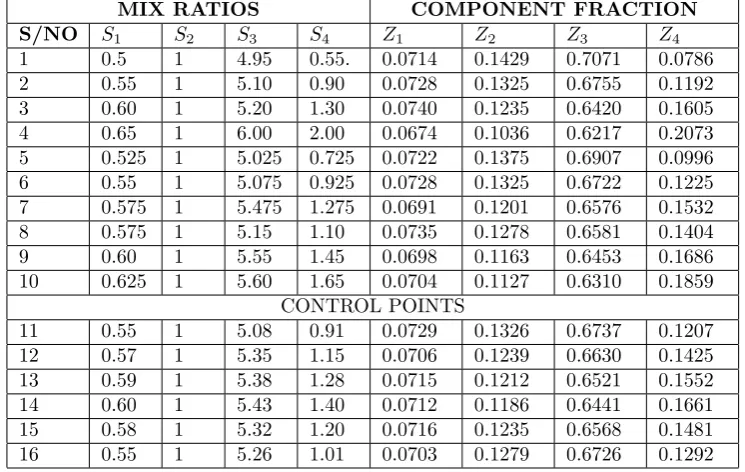
Table 3: Selected mix ratios and components fraction based on osadebes second degree polynomial.
MIX RATIOS COMPONENT FRACTION
S/NO S1 S2 S3 S4 Z1 Z2 Z3 Z4
1 0.5 1 4.95 0.55. 0.0714 0.1429 0.7071 0.0786
2 0.55 1 5.10 0.90 0.0728 0.1325 0.6755 0.1192
3 0.60 1 5.20 1.30 0.0740 0.1235 0.6420 0.1605
4 0.65 1 6.00 2.00 0.0674 0.1036 0.6217 0.2073
5 0.525 1 5.025 0.725 0.0722 0.1375 0.6907 0.0996
6 0.55 1 5.075 0.925 0.0728 0.1325 0.6722 0.1225
7 0.575 1 5.475 1.275 0.0691 0.1201 0.6576 0.1532
8 0.575 1 5.15 1.10 0.0735 0.1278 0.6581 0.1404
9 0.60 1 5.55 1.45 0.0698 0.1163 0.6453 0.1686
10 0.625 1 5.60 1.65 0.0704 0.1127 0.6310 0.1859
CONTROL POINTS
11 0.55 1 5.08 0.91 0.0729 0.1326 0.6737 0.1207
12 0.57 1 5.35 1.15 0.0706 0.1239 0.6630 0.1425
13 0.59 1 5.38 1.28 0.0715 0.1212 0.6521 0.1552
14 0.60 1 5.43 1.40 0.0712 0.1186 0.6441 0.1661
15 0.58 1 5.32 1.20 0.0716 0.1235 0.6568 0.1481
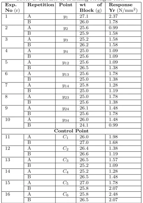
Table 4: Results of crushing strength test.
Exp. No(r)
Repetition Point wt of Block(g)
Response Yr(N/mm2)
1 A y1 27.1 2.37
B 26.0 1.78
2 A y2 25.6 0.99
B 25.9 1.58
3 A y3 25.2 1.58
B 26.2 1.58
4 A y4 25.0 1.09
B 25.6 1.09
5 A y12 25.6 1.09
B 26.5 1.38
6 A y13 25.6 1.78
B 25.0 1.38
7 A y14 25.8 1.28
B 25.0 1.19
8 A y23 25.0 1.78
B 25.6 1.38
9 A y24 26.1 1.48
B 25.6 1.78
10 A y34 26.0 1.48
B 24.1 0.99
Control Point
11 A C1 26.0 1.98
B 27.0 1.68
12 A C2 26.4 1.38
B 26.6 1.19
13 A C3 26.5 1.57
B 25.2 1.09
14 A C4 25.2 1.28
B 26.5 1.48
15 A C5 27.0 1.78
B 25.8 2.07
16 A C6 25.8 2.48
B 26.5 2.07
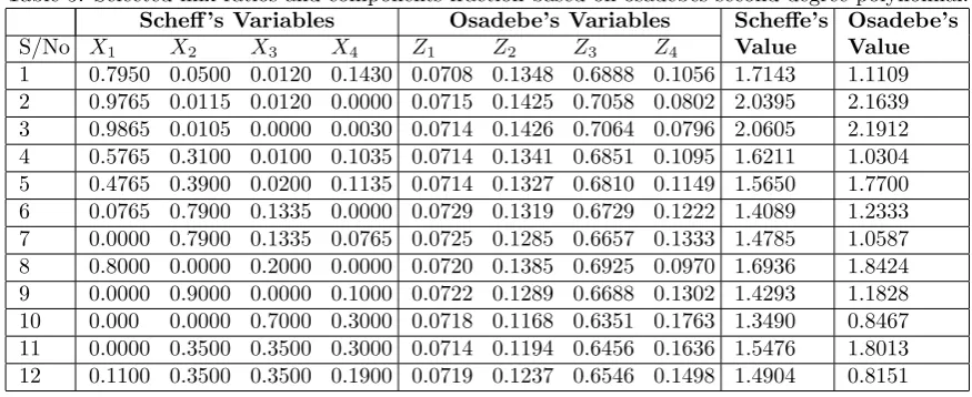
6.2. Comparison of strength values predicted by the two optimization models
Predicted strength values for compressive strength based on Scheffe’s and Osadebe’s sec-ond degree model equations are shown in Ta-ble 5.
6.3. Adequacy test for the models
A statistical adequacy test for the mathe-matical models is necessary. For this the sta-tistical hypothesis is used as
follows:-i. Null hypothesis, H0: There is no
signifi-cant difference between the two models. ii. Alternative hypothesis, H1: There is a
significant difference between the two models. The results of predictions were compara-tively analysed using the statistical package for social sciences (SPSS) for the student’s t -test. The results shows that tcal = 1.9 using
paired-samples T-test in SPSS. >
At α = .05, df 11, Ttable = 2.20. Since,
Ttable > Tcal It shows that there is no
signifi-cant different between the two models so the two models are acceptable for the prediction of compressive strength of sandcrete blocks.
7. Conclusion
It has been shown from this work that Scheffe’s simplex lattice theory and Osadebe’s optimization theory for mixture design have been successfully applied in generating a mathematical models for the compressive strength of sandcrete block as a multivariate function of the proportions of its constituents ingredients: water, cement, sand and laterite fines.
Scheffe’s model was established in the form
y = f(x1, x2, x3, x4) where x1, x2, x3, and
x4 are in the pseudo-components ratio and
Os-adebe’s model in the form of f(z1, z2, z3, z4)
where z1, x2, z3, and z4 are real
Table 5: Selected mix ratios and components fraction based on osadebes second degree polynomial.
Scheff ’s Variables Osadebe’s Variables Scheffe’s Osadebe’s
S/No X1 X2 X3 X4 Z1 Z2 Z3 Z4 Value Value
1 0.7950 0.0500 0.0120 0.1430 0.0708 0.1348 0.6888 0.1056 1.7143 1.1109
2 0.9765 0.0115 0.0120 0.0000 0.0715 0.1425 0.7058 0.0802 2.0395 2.1639
3 0.9865 0.0105 0.0000 0.0030 0.0714 0.1426 0.7064 0.0796 2.0605 2.1912
4 0.5765 0.3100 0.0100 0.1035 0.0714 0.1341 0.6851 0.1095 1.6211 1.0304
5 0.4765 0.3900 0.0200 0.1135 0.0714 0.1327 0.6810 0.1149 1.5650 1.7700
6 0.0765 0.7900 0.1335 0.0000 0.0729 0.1319 0.6729 0.1222 1.4089 1.2333
7 0.0000 0.7900 0.1335 0.0765 0.0725 0.1285 0.6657 0.1333 1.4785 1.0587
8 0.8000 0.0000 0.2000 0.0000 0.0720 0.1385 0.6925 0.0970 1.6936 1.8424
9 0.0000 0.9000 0.0000 0.1000 0.0722 0.1289 0.6688 0.1302 1.4293 1.1828
10 0.000 0.0000 0.7000 0.3000 0.0718 0.1168 0.6351 0.1763 1.3490 0.8467
11 0.0000 0.3500 0.3500 0.3000 0.0714 0.1194 0.6456 0.1636 1.5476 1.8013
12 0.1100 0.3500 0.3500 0.1900 0.0719 0.1237 0.6546 0.1498 1.4904 0.8151
maximum mean strength obtained in Scheffes model is 2.07N/mm2 which is in agreement
with earlier results by Osilli [10]. From this result, it can be concluded that Osadebe’s model can also be used as it is easier to ap-ply because it uses actual mix ratio instead of the pseudo-components ratio that needs to be transformed into real component ratio in Scheffe’s model. Adequate test shows sec-ond degree polynomial can model the response surface with very high degrees of accuracy us-ing the two models.
References
1. Popovics and J. Ujhelyi (2008). Contribution to the concrete strength versus water-cement ratio relationship. J.mater. civil Eng, 20. 459-463.
2. Jee, N, Y Sangehun and C Hongbum, (2004). Prediction of compressive strength of in situ con-crete based on mixture proportions. J. Asian Architect. Build. Eng., 3 9–16.
3. M.F.M. Zain and S.M. Abd (2009). Multiple re-gression model for compressive strength predic-tion of high performance concrete. J. of Applied Sciences, 9(1), pp 155–160.
4. J. A. Cornell,(1990). Experiments with tures; designs, models, and the analysis of mix-ture data, 2nd ed.,John wiley & Sons, New York-Toronto .
5. Akhanzarova, S. and Kafarove, V,(1982). Exper-iment Optimization on Chemisty and Chemical Engr; Translated from Russian by Matskovsky,
Vla Dimir, M. And Repyers, A, Muscow: MIR Publishers. pp 240 248.
6. Scheffe, H .(1958). Experiments with Mixtures. Journal of the Royal Statistical Society, Ser. R. 20 (1958) pp. 344 360
7. Akpuokwe, C.V,(1996). A Computer Model
for Optimization in Concrete Mix proportioning, Project Report (B. Engr). University of Nigeria, Nsukka.
8. Obam, S.O. (2007). Mathematical models for optimization of the mechanical properties of con-crete made from rice husk ash.PhD thesis, Civil Engineering Department ,university of Nigeria, Nsukka.
9. Nwakonobi, T.U,(1997). A Computer Optimiza-tion Model for Mix ProporOptimiza-tioning of Clay - Rice Husk - Cement Mixture for Partition Walls of Animal Building, Project Report (M. Engr) Uni-versity of Nigeria, Nsukka .
10. Neville A.M (1981),Properties of Concrete. The English Language Book Society and Pitman, 1981, p: 118-201.