Vol. 7, No. 1, 2014, 41-46
ISSN: 2279-087X (P), 2279-0888(online) Published on 9 September 2014
www.researchmathsci.org
Annals of
Solid Transportation Problem Under Budget Constraint
Using Fuzzy Measure
Pravash Kumar Giri 1, Manas Kumar Maiti 2 and Manoranjan Maiti 1 1
Department of Applied Mathematics with Oceanology and Computer Programming, Vidyasagar University, Medinipore-721102, India
E-mail: pragiri [email protected]; [email protected]
2
Department of Mathematics, Mahishadal Raj College, Mahishadal Purba Medinipur-721628, India, E-mail: [email protected]
Received 1 August 2014; accepted 20 August 2014
Abstract. Fixed charge solid transportation problems are formulated under a budget
constraint at each destination. Unit transportation costs, fixed charges, sources at origins, demands at destinations, conveyances capacities are assumed to be crisp or fuzzy. Budget constraints at destinations are imposed. It is also assumed that transported units are crisp. So the problem is formulated as constraint optimization programming problem in crisp and fuzzy environments. As optimization of fuzzy objective as well as consideration of fuzzy constraint is not well defined, credibility of fuzzy event are used to transform the problem into equivalent crisp problem. The reduced crisp problem is solved following Generalized Reduced Gradient (GRG) method using lingo software. The models are illustrated with numerical examples.
Keywords: Solid Transportation Problem, Budget constraints, Credibility measure
AMS Mathematics Subject Classification (2010): 90B05
1. Introduction
charge STP and developed algorithms to solve the problem using credibility measures on fuzzy sets.
From above discussions there are some lacunas in the existing STP models, which are summarized below.
• Transportation problems-TP or STP are normally formulated and solved as cost minimization problems, very few might have formulated these as fuzzy fixed charge cost minimization problems.
• In the literature, there are several research works on transportation with uncertain sources, demands, conveyances capacities, etc. None has investigated FCSTP under destination budget constraints with transportation costs, fixed charges, etc.
Overcoming the above mentioned shortcomings, here we have considered cost minimization FCSTP under destination budget constraints with crisp and fuzzy data. In this paper, crisp and fuzzy FCSTPs are formulated as cost minimization problems under fuzzy resource (budget) constraints. The fuzzy objective and constraints are transformed to equivalent crisp forms using credibility measures. The above transportation problems are solved by generalized reduced gradient (GRG) method. The methods are illustrated with numerical examples.
2. Preliminaries
2.1. Credibility measure
Credibility measure was presented by Liu and Liu [6]. For a fuzzy variable with membership function μ(x) and then for any set B⊂R of real numbers, credibility measure of fuzzy event { ∈ B} is defined as Cr{∈ B} =( 1 /2)(Pos ∈ B}+Nec ∈ B}), where possibility and necessity measures of ∈ B} are respectively defined as
∈ ∈ μ(x) ) and
∈ 1 ∈^ μ(x)
2. 2. Optimistic and pessimistic value (Liu[5])
Let be a fuzzy variable and β∈ 0,1!. Then β-optimistic value of is denoted by
"#$ %&d is defined as
'() "#$ sup- . /- 0 - 0 1
and Similarly β- pessimistic value of is denoted by 234"#$ %&d is defined as
567"8$ inf- . /- < - 0 1
Lemma 1. Let =(%=, %>, %?) be a triangular fuzzy number. Then β-optimistic value is
"#$ 21 %>A "1 2β$a? DE β < 0.5
"#$ "21 1$%=A 2"1 β$a> DE β H 0.5
234"#$ 2"1 1$%>A "2β 1$ a? DE β H 0.5
3. Proposed FCSTPs with budget constraints 3.1. Assumptions and notations
In order to construct the mathematical model for the unbalanced FCSTPs under destination budget constraints, the following notations are introduced:
(i) M : number of origins/sources of the transportation problem. (ii) N : number of destinations/demands of the transportation problem. (iii) K: number of conveyances i.e. different modes of transporting units from sources to destinations. (iv) IJ: amount of
homogeneous product available at the i-th origin. (v) KL : demand at the j-th destination.
(vi) MN: amount of the product which can be carried by k-th conveyance. (vii) OJLN: per
unit transportation cost from i-th origin to j-th destination by k-th conveyance. (viii) PJLN:
fixed transportation charge for transporting units from i-th origin to j-th destination by k-th conveyance. (ix) x5RS: the amount transported from i-th origin to j-th destination by
k-th conveyance.
Symbol ˜ is used with the above notations to represent corresponding fuzzy parameters. If the transportation activity is assigned from source i to destination j by conveyance k, then the fixed charge will be costed. This implies that if x5RS > 0 we must add the fixed charge
to the total transportation cost. Thus for the convenience of modelling, the following notation is introduced: y5RS =1 for x5RS 0 0, 0, otherwise.
3.2. Mathematical model formulation
Model-I (Crisp Model): In this model, fixed charge and unit transportation cost are
crisp. Sources, destinations, conveyances capacities of transportation problem are also taken as crisp. So the problem mathematically takes the following form
Minimize Z ∑ ∑ ∑ C5RS= x
5RSA f5RS y5RS
\ S]= ^ R]= _
5]=
Subject to ∑ ∑\ x5RS
S]= ^
R]= < A5 "i 1,2, … , M$
∑_5]=∑\S]=x5RS 0 BR "j 1,2, … , N$
∑_5]=∑^R]=x5RS < ES "k 1,2, … , K$
∑_5]=∑ C^R]= 5RS= x5RSA f5RSy5RS< BudR
x5RS0 0
Model-II (Fuzzy Model): In this model, fixed charge and unit transportation cost are
fuzzy. Sources, destinations, conveyances capacities of transportation problem are also taken as fuzzy. So the above problem mathematically takes the following form:
Minimize Z ∑ ∑ ∑ C5RS= x
5RSA f5RSy5RS
\ S]= ^ R]= _
5]=
=(n=, n>, n?)
∑ ∑\ x5RS
S]= _
5]= 0 BR "j 1,2, … , N$
∑_5]=∑^R]=x5RS < ES "k 1,2, … , K$
∑ ∑ C5RS= x
5RSA f5RS y5RS ^
R]= _
5]= < BudR
x5RS0 0
4. Deterministic equivalent of imprecise model
Till date, for the best of our knowledge, optimization of fuzzy objectives with fuzzy constraints are not well defined. As a result Model-II can not be solved in the present form. Deterministic equivalent of model-II can be derived in the following approach. Here credibility measure is used, which is discussed below.
Model-IIA
Minimize f
Subject to Crp"Z=, Z>, Z?$ < fq 0β
Crp∑^R]=∑\S]=x5RS< A5q 0β "i 1,2, … , M$
Crp ∑_5]=∑\S]=x5RS0 BRq 0β "j 1,2, … , N$
Crp∑ ∑^ x5RS< ES
R]= _
5]= q 0β "k 1,2, … , K$
Crp ZR< BudRq 0β
x5RS0 0
Model-IIA-1: When DM is optimistic, then he/she assumes value of β≤ 0.5 i.e. (0 ≤β≤
0.5) and hence using lemma-1,-2 , the Model-IIA reduces to Minimize O==(1-2β) Z=+2βZ>
Subject to ∑^R]=∑\S]=x5RS< 2βA5>A "1 2B$A5? "i 1,2, … , M$
∑5]=_ ∑S]=\ x5RS 0 "1 2β$BR=A 2βBR> "j 1,2, … , N$
∑5]=_ ∑R]=^ x5RS < 2βES>A "1 2β$ES? "k 1,2, … , K$
"1 2β$ZR=A 2βZR> < BudR
x5RS0 0
Model-IIA-2: When DM is pessimistic, then he/she assumes value of β≥ 0.5 i.e. (0.5 ≤β ≤ 1) and hence using lemmas-1,-2 , the Model-IIA reduces to
Minimize s>=2(1-β) n>+(2β-1) n?
Subject to ∑R]=^ ∑S]=\ x5RS< "2β 1$A5>A 2"1 β$A5? "i 1,2, … , M$
∑5]=_ ∑S]=\ x5RS 0 2"1 β$BR=A "2β 1$BR> "j 1,2, … , N$
∑5]=_ ∑R]=^ x5RS < "2β 1$ES>A 2"1 β$ES? "k 1,2, … , K$
2"1 β$ZR=A "2β 1$ZR> < BudR
x5RS0 0
5. Numerical experiment
5.1. Input data
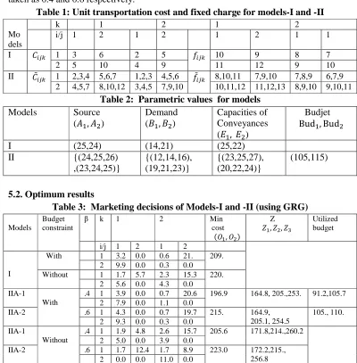
For both models, no of origins=2 (i.e. M=2), no of destination=2 (i.e. N=2), no of conveyance=2 (i.e. K=2) are considered. Crisp and fuzzy unit transportation costs and fixed charges for Models-I and -II are given in Table-1. Parametric values for models are presented in Table-2. Credibility measure of constraints and objective, values of β are taken as 0.4 and 0.6 respectively.
Table 1: Unit transportation cost and fixed charge for models-I and -II
Mo dels
k 1 2 1 2
i/j 1 2 1 2 1 2 1 1
I /2tu 1 3 6 2 5 E2tu 10 9 8 7
2 5 10 4 9 11 12 9 10
II /2tu 1 2,3,4 5,6,7 1,2,3 4,5,6 E2tu 8,10,11 7,9,10 7,8,9 6,7,9
2 4,5,7 8,10,12 3,4,5 7,9,10 10,11,12 11,12,13 8,9,10 9,10,11
Table 2: Parametric values for models
Models Source
(=, >)
Demand (=, >)
Capacities of Conveyances (v=, v>)
Budjet Bud=, Bud>
I (25,24) (14,21) (25,22)
II {(24,25,26)
,(23,24,25)}
{(12,14,16), (19,21,23)}
{(23,25,27), (20,22,24)}
(105,115)
5.2. Optimum results
Table 3: Marketing decisions of Models-I and -II (using GRG)
Models
Budget constraint
β k 1 2 Min
cost "s=, s>$
Z n=, n>, n?
Utilized budget
i/j 1 2 1 2
I
With 1 3.2 0.0 0.6 21. 209. 2 9.9 0.0 0.3 0.0
Without 1 1.7 5.7 2.3 15.3 220. 2 5.6 0.0 4.3 0.0
IIA-1
With
.4 1 3.9 0.0 0.7 20.6 196.9 164.8, 205.,253. 91.2,105.7 2 7.9 0.0 1.1 0.0
IIA-2 .6 1 4.3 0.0 0.7 19.7 215. 164.9, 205.1, 254.5
105., 110. 2 9.3 0.0 0.3 0.0
IIA-1
Without
.4 1 1.9 4.8 2.6 15.7 205.6 171.8,214.,260.2 2 5.0 0.0 3.9 0.0
IIA-2 .6 1 1.7 12.4 1.7 8.9 223.0 172.2,215., 256.8 2 0.0 0.0 11.0 0.0
6. Discussion
This paper presents fuzzy cost minimization FCSTPs under budget constraints at destinations with credibility measure. Several examples are used for the illustration. Table-3 furnish the results of crisp (Model-I) and fuzzy (Model-II) cost minimization FCSTP respectively following credibility approach. These results are without and with budget constraints. In all cases, it is observed from Table-3 that minimum cost for the models without budget constraint are more than those with budget constraints. To mention one case, in Table-3, say the minimum cost without budget constraint is 220. $ which is more than the minimum cost (209. $ ) with budget constraint. This is as per the usual expectation.
In Tables-3, lowest cost of all the models, IIA-1 and -2 models, give the lowest and highest minimum cost respectively. This is because both fuzzy objective function and transportation constraints have been changed by the credibility measures (average of possibility and necessity measures) in the ranges (0.0-0.5) and (0.5-1.0)for 1 and IIA-2 respectively.
REFERENCES
1. J.Gottlieb and L.Paulmann, Genetic algorithms for the fixed charge transportation problems in: Proceedings of the IEEE Conf. Evol. Comp., ICEC, 1998, 330-335. 2. K.B.Haley, The solid transportation problem, Oper. Res., 11 (1962) 446-448.
3. W.M.Hirsch and G.B.Dantzig, The fixed charge transportation problem, Naval
Research Logistics Q., 15 (1968) 413-424.
4. F.L.Hitchcock, The distribution of the product from several sources to numerous localities, Journal of Mathematical Physics, 20 (1941) 224-230.
5. B.Liu, Theory and Practice of Uncertain Prog., Physica-Verlag, Heidelberg, 2002. 6. B.Liu and Y.K.Liu, Expected value of the fuzzy variable and fuzzy expected value
models, IEEE Transactions on Fuzzy Systems, 10 (2002) 445-450.
7. E.D.Schell, Distribution of a product by several properties, in: Proceedings of 2nd
Symposium in Linear Programming, DCS/comptroller, HQ US Air Force,
Washington DC, 1955, 615-642.
8. L.Yang and L.Liu, Fuzzy fixed charge solid transportation problem and algorithm,