A Survey on Omega Polynomial of Some Nano Structures

IJMC

A

Survey

on

Omega

Polynomial

of

Some

Nano

Structures

MODJTABA GHORBANI

Department of Mathematics, Faculty of Science, Shahid Rajaee Teacher Training University, Tehran, 16785-136, I. R. Iran

(Received September 1, 2011)

A

A counting polynomial C(G , x) is a sequence description of a topological property so that the exponents express the extent of its partitions while the coefficients are related to the occurrence of these partitions. Basic definitions and properties of the Omega polynomial

) , (G x

 and the Sadhana polynomial Sd(G,x) are presented. These polynomials for some infinite classes of fullerenes and nanotubes are also computed. The results of this paper are arranged according to the main Theorems of [9 43].

Keywords: Omega polynomial, Sadhana polynomial, fullerene, nanotube.

1.

I

Mathematical calculations are absolutely necessary to explore important concepts in chemistry. Mathematical chemistry is a branch of theoretical chemistry for discussion and prediction of the molecular structure using mathematical methods without necessarily referring to quantum mechanics. Chemical graph theory is an important tool for studying molecular structures. This theory had an important effect on the development of the chemical sciences.

A graph can be described by: a connection table, a sequence of numbers, a derived number (called sometimes a topological index), a matrix, or a polynomial [1].

A finite sequence of some graph-theoretical categories/properties, such as the distance degree sequence or the sequence of the number of k-independent edge sets, can be described by so-called counting polynomials:



G

P( , ) ( , ) (1)

where p(G,k) is the frequency of occurrence of the property partitions of G, of length k, and x is simply a parameter to hold k.

Counting polynomials were introduced, in the Mathematical Chemistry literature, by Hosoya with his Z-counting (independent edge sets) and the distance degree polynomials, where initially called Wiener and later Hosoya polynomials [2]. Their roots and coefficients are used for the characterization of topological nature of hydrocarbons.

Hosoya proposed the sextet polynomial [3,4]for counting the resonant rings in a benzenoid molecule. The sextet polynomial is important in connection to the Clar aromatic sextets [5,6] expected to stabilize the aromatic molecules.

The independence polynomial [7, 8] counts the number of distinct k-element independent vertex sets of G. Other related graph polynomials are the king, color and

star or clique polynomials [9].

Vertex contributions to a polynomial P(G,x), based on distance counting, can be written as:



 _{kp i k x}k

x i

P( , ) (1/2) (, ) (2)

Where p(i,k) is the contribution of vertex i to the partition p(G,k) of the global molecular property P=P(G). Note that p(i,k)’s are just the entries in LM or SM, more exactly 1/2 the value because each vertex contribution is counted twice [10].

Usually, the vertex contribution varies from one atom to another, so that the polynomial for the whole graph is obtained by summing all vertex contributions:



 _iP i x x

G

P( , ) (, ) (3)

In a vertex transitive graph, the vertex contribution is simply multiplied by N:

) , ( )

,

(G x N P i x

P   (4)

Hence, P(G) is easily obtained as the polynomial value in x=1: 1 | ) , ( )

(G  P G x _x

P (5)

A distanceextended property D_P(G) can be calculated by the first derivative of the polynomial in x = 1 [11  15]:

1 1_| ) , ( ) , ( ) (

_   



k x k G p k x G P G P

D (6)

In [16], the authors produced a treatment apparently independent of Hosoya's. Perhaps the most interesting property of H(G,x) is the first derivative, evaluated at x = 1, which equals the Wiener index: H G( ,1)W G( ). Ashrafi [17]continued the line of the mentioned paper of Sagan et al. to introduce the notion of PI polynomial of a molecular graph G as:

( , ) ( , ) ( )

( , ) N u v

u v e E G

PI G x x

 





the edge e = uv E(G) is given by: N e( ) E G( )N u v( , ), where E(G) denotes the set of all edges of the graph G. In [17] the authors have shown that this new polynomial has the same basic properties as the Wiener polynomial. Thus, its first derivative gives the PI index, which can also be calculated by subtracting the total number of equidistant edges in G from the square of the edge set cardinality:

 

( ) ( ,1) _e ( )

PI G PI G  E 



See also [18  20] for more details about PI index. Here, our notations are standard and taken from [21  23]. The basic definitions and properties of the Omega polynomial

) , (G x

 are presented in the second section. In the third section the Omega polynomial of some wellknown graphs are computed.

2.

M

R

A

D

We now recall some algebraic definitions that will be used in the paper. Let G be a simple molecular graph without directed and multiple edges and without loops, the vertex and edge-sets of which are represented by V(G) and E(G), respectively. Throughout this paper, graph means simple connected graph. The vertex and edge sets of a graph G are denoted by V(G) and E(G), respectively. If x, yV(G) then the distance

d(x, y) between x and y is defined as the length of a minimum path connecting x and y.

2.1 OMEGA POLYNOMIAL

The Omega polynomial is a counting polynomial introduced by M. V. Diudea. In recent years, several papers on methods for computing Omega polynomials of molecular graphs have been published [24 – 43].

Let G be a connected bipartite graph with the vertex set V V G ( ) and edge set

( )

EE G , without loops. Two edges e = ab and f = xy of G are called co-distant

(briefly: e co f) if for k = 0,1,2,… there exist the relations: d(a,x) = d(b,y) = k and d(a,y) = d(b,x) = k+1 or vice versa. For some edges of a connected graph G there are the following relations satisfied:

e co f (9)

e co ff co e (10)

e co f & f co ge co g (11)

though, the relation (11) is not always valid.

Let C(e):= {e'E G( ); e’ co e } denote the set of all edges of G which are co-distant to the edge e. If all the elements of C(e) satisfy the relations (911) then C(e) is called an orthogonal cut “oc” of the graph G. The graph G is called co-graph if and only if the edge set E(G) is the union of disjoint orthogonal cuts: C₁C₂ ... C_k E

and CiCj Ø for i j, i,j1,2,...,k.

Suppose T denotes the outside edges of G. Start with an edge e of G. If there is not an edge e1 different from e with the property that e co e1 and {e,e1} lie in the same face of

G then we define H= {e1} and choose another edge f of G. Otherwise, there exists the

edge e1 such that e co e1. Continue this process by e1 to construct the sequence e co e1

co e2 co … co er. If e  T then define H = {e, e1, e2, …,er}. If not, there exists an edge f1

of G different from e1 such that f1 co e and {e,f1} lie in the same face of G. By this

algorithm a sequence H= {ft, …, f1, e, e1, e2, …, er} is constructed. H is called a

quasiorthogonal cut or a qoc strip. It is an easy fact that a qoc strip is not necessarily transitive. In the case that G is bipartite, then every member of S have an even number of edges and so ft, er T. Notice that a qoc strip starts and ends either out of G (at an

edge with endpoints of degree lower than 3, if G is an open lattice,) or in the same starting polygon (if G is a closed lattice). Any oc strip is a qoc strip but the reverse is not always true.

Suppose E1, E2, …,Er are qoc strips of a connected planar bipartite graph G. We

claim that X = {E1, E2, …,Er} is a partition of E = E(G). To do this we assume that e 

E is an arbitrary edge of G. Using a similar argument as those given above one can find a sequence ft co ft-1 co … co f1 co e co e1 … co er. Therefore there exists j, 1 ≤ j ≤ r, such

that {ft, …, f1, e, e1, …, er}  Ej. This implies that e Ej and so E = E1 E2 … Er. To

complete our claim, we must prove EiEj = , for 1 ≤ i j ≤ r. Suppose Ei = {e1,e2, …,

en}, Ej = {f1,f2,…,fm} and e Ei  Ej. Then there are r, s, 1 ≤ r ≤ n and 1 ≤ s ≤ m such

that e = er = fs. But every edge appears in at most two members of S, so by using an

inductive argument Ei = Ej. Therefore, X is a partition of E.

The OmegaΩ(G,x)polynomial for counting qoc strips in G is defined as:

( , ) ( , ) c

Ω G x _cm G c x (12)

with m(G,c) being the number of strips of length c. The summation runs up to the maximum length of qoc strips in G.

If G is bipartite then a qoc starts and ends out of G and so Ω(G,1)r/2,in which r is the number of edges in out of G. On the other hand, one can easily seen that

( ,1) ( )

c

G m c e E G



 



) , (G x

Ω as:

1

2 _{( )}

) ( )

(G  Ω  ΩΩ _x

CI (13) 1 / 1 )) , ( ( )) , ( / 1 ( )

(   



Ω G Ω G x Ω G x

I (14)

In case of I_, summation runs over all possible derivatives d in the corresponding polynomial. When one or more edges do not belong to a counted strip, such edges are added as “strips of length 1”.

It is easily seen that, for a single qoc, one calculates the polynomial: ( , )G x xc

  and CI G( )c2 (c c c( 1)) 0 . There exist graphs for which CI equals

evaluation in the graph involves only the locally parallel edges. This is occurred for example in partial cubes. In this case, we have:

2 2 2

( )

(

) [

]

c c c c

CI G 









This counting polynomial is useful in topological description of benzenoid, structures as well as in counting some single number descriptors, i.e., topological indices. The qoc strips could give account for the helicity of polyhex nanotubes and nanotori. The Omega 1.1 software program includes the qoc strips procedure.

In the end of this section a simple counterexample for equations (9-11) is given in Figure 1. In the graph G1; {a} and {c} are oc strips; {b} and {d} does not have all elements co-distant to each other, so that {b} and {d} are qoc strips. In the graph G2;

{a} and {b} and {c} are oc strips; {f} and {c} are equidistant but {f} and {c1 or c3} do not obey the symmetry relation (8) (and do not belong to one face) thus {f} does not belong to the strip {c}. Therefore, Ω(G₁,x)x22x4x6and 2 3

2, ) 5 2

(G x x x x

Ω   

.

Figure 1. Two Graphs G1 (left) and G2 (right).

2.2 EXAMPLES

In this section the Omega polynomial of some well-known graphs are computed. A general formula for computing Omega polynomial of the graph product is presented by which, it is possible to compute the Omega polynomials of nanotubes and nanotori covered by C4. We begin by some well-known graphs.

Example 1.Suppose Tn, Cn and Kn denote the an arbitrary acyclic graph, cycle and

complete graph on n vertices, respectively. Then by simple calculations, one can see that ( ) | ( , ) , | n n n n n

x x n

K x nx n        _{ }   _  1 2 2 1 2 2 2 2 | ( , ) | n n x n C x nx n    _{ }  _  2 ₂ 2 2

and(T,x) = (n1)x.

The Cartesian product G  H of graphs G and H is a graph such that V(G  H) =

either a = u and b is adjacent with v, or b = v and a is adjacent with u. The following properties of the Cartesian product of graphs are crucial:

(a) |V (G × H)| = |V(G)| |V(H)| and |E(G × H)| = |E(G)| |V(H)| + |V(G)| |E(H)|;

(b) G × H is connected if and only if G and H are connected;

(c) If (a, x) and (b, y) are vertices of G × H then dG×H((a, x), (b, y)) = dG(a, b) +

dH(x,y);

(d) The Cartesian product is associative.

Theorem 2. Let G and H be bipartite connected co-graphs. Then

1 2

1 2

| V (H ) | | V (G ) |

1 2

( , ) ( , ). c ( , ). c .

c c

Ω G H x 





Proof. Suppose that for an edge e = uv of an arbitrary graph L, NL(e) = |E| − (nu(e) + nv(e)). Then by definition,

G×H

|V (G)| N ( f ) for a = b and x y = f E(H ) N ((a, x), (b, y)) =

|V (H)| N ( g ) for x = y and ab = g E(G).

 

 _



By above paragraph and definition of the Omega polynomial, we have:

1 2

1 1 2 2

( , ) ( , ). c ( , ). | V (H ) | c ( , ). | V (G ) | c

c c c

Ω G H x 







which completes the proof.

Corollary 3. Let G , G , · · · , G _{1 2 n} be bipartite connected co-graphs. Then we have:

j 1

| V (G ) |

1 2 n

1

(G × G × · · · × G , ) ( , ). n i j j i i c n i i c i

Ω x m G c x 









Proof. Use induction on n. By Theorem 2.2, the result is valid for n = 2. Let n ≥ 3 and

assume the theorem holds for n - 1. Set G = G1 × · · · × Gn-1. Then we have | V ( ) | | V (G ) |

( , ) ( , ). n ( , ). n

n

G c c

n c c n n

Ω G G x 





= 1 1 1 ( , ). ( , ). n j i j

j i n

i n

| V (G ) | c n

| V (G ) | c

i i n n

c c

i

m G c x  m G c x

   





| V (G ) | c n

i i c

i

m G c x 







Example 4. In this example the Omega polynomial of nanotubes and nanotori covered

by C4 are calculated. By definitions of Cartesian product of graphs and Omega polynomial, one can easily prove:

1 2

1 2

| V (H ) | | V (G ) |

1 2

( , ) ( , ) c ( , ) c

c c

Suppose R and S denote a C4tube and C4torus, respectively. Then by definition

R  Pn  Cm and S  Ck  Cm. Apply Theorem 2 to deduce that

( , ) ( 1) m ( 1) n n m

P P x n x m x

      . On the other hand, we have:

2

( 1) 2|m

2

( , )

( 1) 2|m

m n

n m

m n

m

n x x

P C x

n x mx

      _{ }     , 2 2 2 2

2|m , 2|n

2|m , 2|n 2

( , ) _n

2|m , 2|n 2

n

2|m , 2|n

2 2

m n

m n

n m _{m n}

m n

nx mx

m

nx x

C C x

x mx m x x     _    _{ }     _  .

Example 5.Consider the molecular graph of a nanocones G = CNC4[n], Figure 2. This

graph has exactly 4(n + 1)2 vertices. From Figure 2, one can see that there are m + 1 type of edges of G. These are I1, I2,… and Im+1. In Table 1, for each type the number of

equidistant edges of Gis computed. By this calculation, we can see that

Ω(G, x) = 2x2m+2 + 4(x2m+1 + x2m +…+ xm+2) = 2x2m+2 + 4(x2m+2xm+2)/(x1).

Table 1.The Number of Parallel Edges.

Edges Number of

Parallel Edges No

Type I1 Edges m+2 4

Type I2 Edges m+3 4

Type I3 Edges m+4 4

  4

Type Im+1 Edges 2m+2 2

In the end of this section, the Omega polynomials of TWHH[p,q](R) nanotubes and nanotori are computed, Figures 35. The molecular graphs of these compounds are denoted by G and H, respectively. From Figures 3-5, one can see that there are two different cases for qoc strips. Suppose e1 and e2 are representatives of the different cases. In the molecular graph G, |C(e1)| = 2p and |C(e2)| = 2q+1. On the other hand, there are q and 2p similar edges for each of edges e1 and e2, respectively. This implies that Ω( , )_{G x qx + 2px}2p 2q+1_{. For the graph H, |C(e}

other hand, there are q and 2 similar edges for the edges e1, e2, respectively. Therefore,

Ω( , )_{H x qx + 2x}2p 2pq_.

Figure 2. The Molecular graph of carbon nanocones CNC4[n].

Figure 3.The qoc strips of the 2dimensional graph of a TWHH[p,q](R) nanotube.

1 2 3 4 . . . . p

1

2

3

q . . .

e₁

e₂

Figure 4.The qoc strips of the nanotube G.

1 2 3 4 . . . . p

1

2

3

q . . .

e1

e2

Figure 5. The qoc strips of the nanotorus H.

1 2 3 4 . . . . p

1

2

3

q . . .

e₁

2.3 OMEGA POLYNOMIAL OF FULLERENES

The fullerene era was started in 1985 with the discovery of a stable C60 cluster and its interpretation as a cage structure with the familiar shape of a soccer ball, by Kroto and his co-authors [44,45]. The well-known fullerene, the C60 molecule, is a closed-cage carbon molecule with three-coordinate carbon atoms tiling the spherical or nearly spherical surface with a truncated icosahedral structure formed by 20 hexagonal and 12 pentagonal rings. Let p, h, n and m be the number of pentagons, hexagons, carbon atoms and bonds between them, in a given fullerene F. Since each atom lies in exactly 3 faces and each edge lies in 2 faces, the number of atoms is n = (5p+6h)/3, the number of edges is m = (5p+6h)/2 = 3/2n and the number of faces is f = p + h. By the Euler’s formula n − m + f = 2, one can deduce that (5p+6h)/3 – (5p+6h)/2 + p + h = 2, and therefore p = 12, v = 2h + 20 and e = 3h + 30. This implies that such molecules made up entirely of n carbon atoms and having 12 pentagonal and (n/2  10) hexagonal faces, where n 22 is a natural number equal or greater than 20.

In this section, the Omega polynomials of some infinite classes of fullerenes are investigated. Begin by small fullerenes C20 and C30 depicted in Figure 6.

a

_b

Figure 6. (a) The fullerene graph C20 (b) The fullerene graph C30.

Then by our method Ω(C20 , x) = 30x and Ω(C30 , x) = 20x + 10x2 + x5. We now compute the Omega of an infinite family of fullerene graphs with 40n + 6 vertices, Figure 7.

Theorem 6. The Omega polynomial of fullerene graph G = C40n+6 is computed as

2 2 1 4 1 4

4 3 2 2 4 4 4 1

2 2 1 4 4 2

2 2 2 2 4 1 4 2

2 2 2 1 2 4 3 8 6

( ) 4 4 4 2 5 |

( ) 2 8 2 2 5 | 1

( , ) ( ) 8 4 2 2 5 | 2

( ) 4 4 4 2 5 | 3

( ) 4 4 4 2 5 | 4

n n n n

n n n n

n n n n

n n n n

n n n n n

a x x x x x n

a x x x x x n

G x a x x x x x n

a x x x x x n

a x x x x x x n

 

   

 

   

   

 _{   }

 

    

  

 _     



 _{    }

 

      



,

where a x( ) x 9x24x32x4(2n3)x10.

Proof. From Figure 7, one can see that there are ten distinct cases of ops strips in G. We

denote the corresponding edges by e1, e2, …,e10. By using calculations given in Table 2 and the Figure 8, the proof is completed.

e

e

e

e

e

e

e

e

e

e

e

Table 2. The number of Codistant edges of ei, 1≤i≤10.

No. Number of Co-Distant Edges Type of Edges

1 1 e1

9 2 e2

4 3 e3

2 4 e4

2n-3 10 e5

2

2 1 5

4 3 5 1

2 5 4 2

2 2 5 3

n n

n n

n n n

n n    _{ }   _{ }     | | | , | e6 2 4 4    

4 1 5 3

2 5 2

2 2 5 1 4

n n

n n n

n n n

    _   _{  }  | | , | , e7 4 4 2    

2 2 5 | 1, 3

2 1 5 | 2, 4

4 1 5 |

n n n

n n n

n n      _{  }   _  e8 1 2 2 2     

8 6 5 4

4 2 5 3

4 4 5 1

4 5 2

n n

n n

n n

n n n

    _{ }   _{ }    | | | | , e9 2

4 1 5 3

4 1 5 1

4 2 5 2

4 3 5 4

n n n

n n n n n n     _{ }   _{ }     | , | | | e10 2

2 1 5

2 5 2 4

2 2 5 3

n n

n n n

Graph of fullerene C40n+6 Edges codistant to e1 Edges codistant to e2

Edges codistant to e3 Edges codistant to e4 Edges codistant to e5

Edges codistant to e6 Edges codistant to e7 Edges codistant to e8

Edges codistant to e9 Edges codistant to e10 Edges codistant to e11

Figure 9. The fullerene graph Fn, n = 8.

Next, we consider a class of fullerenes with exactly 10n vertices, Figure 9. From Figure 10, there are six distinct cases of qoc strips as follows:

e1 e2 e3

e4 e5 e6

We denote the corresponding edges by e1, e2, …,e6. Then |C(e1)| = |C(e2)| = |C(e3)| = |C(e6)| = 1, |C(e4)| = 5 and |C(e5)| = n – 1. On the other hand there are five similar edges for each of edges e1, e2, e3 and e6, n – 2 edges similar to e4 and 10 edges similar to

e5. Therefore,

5 ( 1)

( , ) 20F x_n x (n 2) x 10 x n

        .

In what follows, a new class of fullerenes with 10n carbon atoms are considered, see Figure 11. In Table 3, we lists the Omega polynomial of Fnfor n 9.

Table 3. The Omega Polynomial of Fn for n  9.

Fullerenes  Polynomials

C20 30x

C30 20x+x5+10x2 C40 20x+2x5+10x3 C50 20x+3x5+10x4 C60 20x+4x5+10x5 C70 20x+5x5+10x6 C80 20x+6x5+10x7 C90 20x+7x5+10x8

Theorem 7. Consider the fullerene graphs C10n, n ≥ 2. Then the Omega polynomial of C10n is computed as follows:

3 ₂ -3

10

-3 3

3 _{2 2} -3

10 10 10 2 |

Ω( , ) ,

10 5 5 10 2 |

n

n

n

n n

n

x x x n

F x

x x x x n





 

   

   



Proof. To compute the Omega polynomial of C10n, it is enough to calculate C(e) for

every e  E(G). In Tables 4 and 5, the number of co-distant edges of this fullerene, are computed. From calculations given in Tables 4, 5 and Figure 11, 12 the equation is obtained which completes the proof.

Table 4.The Number of Co-Distant Edges, when 2|n.

Type of Edges Number of Co-Distant Edges No

e1 3 10

e2 n/2 10

Table 5.The Number of Co-Distant Edges,when2 |n.

Type of Edges

Number of Co-Distant

Edges

No

e1 3 10

e2 3

2 n

5

e3 3

2 n

5

e4 n  3 10

e

e

e

e

e

e

e

Figure 12. The fullerene graph C10n (n is even).

Theorem 8.Suppose G is the molecular graph of C24n fullerene. Then the Omega

polynomial of G is( , ) 3G x  x2n6xn12x2n312 .x3

Proof. It is easy to see that there are four different type of edges, f1, f2, f3 and f4, Figure

13. The number of edges codistant to f1, f2, f3 and f4 are 2n, 2n-3, 3 and n, respectively. On the other hand, there are 3 edges similar to f1, 12 edges similar to f2, 12 edges similar to f3 and 6 edges similar to f4, Figure 13. Therefore,

2 2 3 3

( , ) 3G x x n 6xn 12x n 12 .x

    

Theorem 9. The omega polynomial of fullerene graph C12n+4(Figure 14) is as follows:

2 6 1

12 4

Ω( , ) 18 4 ( 2) 8 n 4 .n

n

C x x x n x x  x

      

Proof. By Figure 15, there are five distinct cases of qoc strips. We denote the

2 6 1 12 4

Ω( , ) 18 4 ( 2) 8 n 4 n.

n

C x x x n x x  x

      

. . .

. .

.

. . .

. .

. .

. .

. .

. f1 f2

f3 f4

Figure 13.The Schlegel graph of C24n fullerene.

. . . . . . . . . . . . . . . . . . . . . . . . . . . . . . . . . . . . . . . . . . . . . . . . . . . . . . . . . . . . . . . . . . . . . . . .

Figure 15. Four different types of edges in C24n Fullerene.

Table 6. The Number of CoDistant Edges of ei, 1 ≤i≤ 5.

No. Number of Co-Distant Edges Type of Edges

4 2 e1

8 n 1 e2

4 n e3

18 1 e4

n 2 6 e5

Theorem 10. The Omega polynomial of the fullerene graph C12(2n+1) is as follows:

3 2 -2 -1 2 4

Proof. By Figure 16, there are four distinct cases of qoc strips. We denote the

corresponding edges by e1, e2, e3 and e4. By table 1 one can see that |C(e1)|=3, |C(e2)| = 2n - 2, |C(e3)| = 2n + 4 and |C(e4)| = n -1. On the other hand, there are 12, 12, 3, and 6 similar edges for each of edges e1, e2, e3, and e4, respectively. So, we have

3 2 -2 -1 2 4

Ω( , ) 12_{G x}  _x 12_x n 6_xn 3_x n , _n2_.

f₁

f₃

f₄

f₂

Figure 16. The qoc strips of edges in graph of fullerene C12(2n+1).

Table 7. The number of co-distant edges of ei, 1 ≤i≤ 4.

Edge The Number of Co

Distant Edges No.

e1 3 12

e2 2n-2 12

e3 2n+4 3

Theorem 11. Let F be a fullerene. Then, ( , 0) 0G  if and only if F be an IPR

fullerene.

Proof. Let ( , 0) 0G  . This implies the multiplicity of x in definition of Omega

polynomial is zero. Since every hexagonal face has 3 strips of length 2, thus none of the pentagons make contact with each other. Conversely, if F be an IPR fullerene, then the length of every strip is greater than 2. Hence, 2

1 2 0

( 0)G, x x ... _x 0 

     .

Lemma 12. Let G be a graph on n vertices, m edges and  be number of its qoc strips.

Then

( ) 1 Sd G

m

   . (15)

Proof. By using definition of Sadhana index we have:

( ) _{s s}(| ( ) | ) _{s s} | ( ) | _{s s} ( 1)

Sd G 







Corollary 13. Let F1 and F2 be fullerenes of order n. Then

1 2 1 2

( ) ( ) ( ) ( )

Sd F Sd F  F  F .

Proof. Since Sd G( ) (  1)m the proof is straightforward. Theorem 14. Suppose F be an IPR fullerene, then

( ) ( 2) / 2. Sd G m m

Proof. For every qoc strip C of F, |C| ≥ 2. Since 2m, thus Sd G( ) 1 m/ 2

m   and so

( ) ( 2) / 2. Sd G m m

Theorem 15.Let F be afullerene graph. Then Sd F( ) (2  '(G_,0)) .m

Proof. Let r and s be the number of qoc strips of length 1 and 2, respectively. Clearly '(0)

r  and since every hexagonal face has at least 3 qoc strips of length 2, thus '

3 ( ,0)G

    . By using equation (15) the proof is completed.

Conjecture 16. Among all of fullerenes F on n vertices the IPR fullerene has the

minimum value of Sd(F).

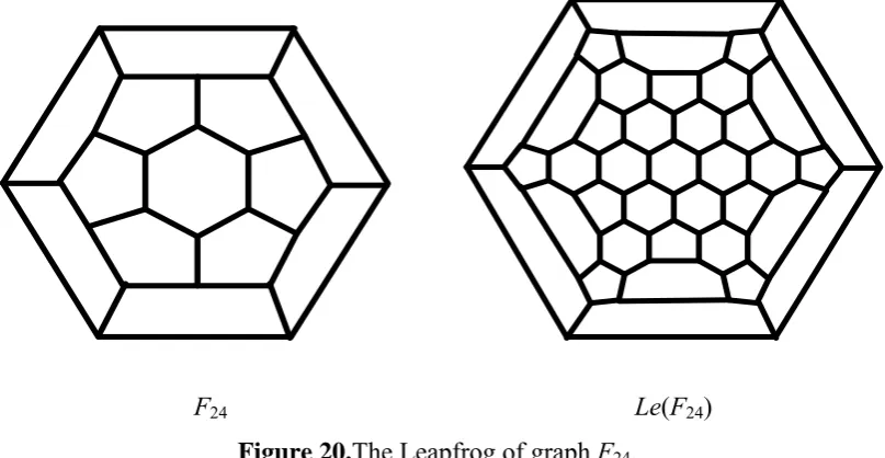
Let G be a fullerene graph on n vertices. A leapfrog transform Gl of G is a graph on 3n vertices obtained by truncating the dual of G. Hence, Gl = Tr(G*), where G*

denotes the dual of G. It is easy to check that Gl itself is a fullerene graph. We say that

Gl is a leapfrog fullerene obtained from G and write Gl =Le(G). In the other word, for a given fullerene Fn put an extra vertex into the centre of each face of Fn. Then connect

hexagonal faces. A sequence of stellationdualization rotates the parent sgonal faces by π/s. Leapfrog operation is illustrated, for a pentagonal face, in Figure 17.

Figure 17. Leapfrog of a pentagonal face.

In Figure 18, one can see that the fullerene graph C20 and its Leapfrog, namely C60. Also, in Figure 19 the 3 dimensional leapfrog graph of C24 and C30 are depicted. We denote the Leapfrog of graph G by Le(F).

Le(C20) = C60.

L(C20) = C60.

Figure 19. Le(C24) and Le(C30).

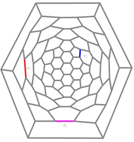
Example 17. Consider the fullerene graph F24 in Figure 20. This fullerene graph has 36 edges. Similar to example 1 one can see that Ω(x) = 24x + 6x2 and so Sd(x)= 24x35 + 6x34. In Figure 20 one can see the planer graphs F24 and Le(F24).

F24 Le(F24)

Figure 20.The Leapfrog of graph F24.

Example 18. Consider the fullerene graph F26 depicted in Figure 21. This fullerene

graph has 39 edges. Similar to examples 1 and 2 one can see that Ω(F26, x) = 21x + 9x2 and so, Sd(F24, x)= 21x38 + 9x37. By computing these polynomials for the Leapfrog fullerene we have:

F26 Le(F26)

Figure 21. The Leapfrog of graph F26.

An automorphism of the graph G = (V, E) is a bijectionσ on V which preserves the edge set e, i. E., if e = uv is an edge, then σ( )e σ( )u σ( )v is an edge of E. Here the image of vertex u is denoted by σ( )u . The set of all automorphisms of G under the composition of mappings forms a group which is denoted by Aut(G). Aut(G) acts transitively on V if for any vertices u and v in V there is αAut G( ) such that α( )u v . Similarly G = (V, E) is called edge-transitive graph if for any two edges e1 = uv and e2 =

xy in E there is an element βA ut G( ) such that β( )e1 e2 where(e1)(u)(v) . Furthermore, if F be a fullerene graph then, Aut(F) = Aut(Le(F)).

As a result of Lemma 32 we compute the Omega polynomial of a hyper – cube. The vertex set of the hypercube Hn consist of all ntuples b1b2…bnwith }bi{0,1 . Two

vertices are adjacent if the corresponding tuples differ in precisely one place. So the hyper – cube Hn has 2n vertices and n.2n-1 edges. On other word, _{n 2 2  2}

n

H K K  _ K .

It is well – known fact that Hn is vertex and edge transitive. We use of this result

and we have the following Theorem:

Theorem 19.(Hn)nx2n1.

Proof. Let e = uv be an arbitrary edge of Hn. By computing the qoc strips one can see that c = |C(e)| = 2n-1. Furthermore, since |E(Hn)| = n.2n-1 the proof is completed.

Now, let G = (V, E) be a graph. If Aut(G) acts edge-transitively on V, then we have the following Lemma:

Lemma 20. Let eE(G) be an arbitrary edge and c = |C(e)|. Then the Omega

| ( ) | Ω(_G,x) E G _xc

c

 .

Proof. Because Aut(G) acts edge-transitively on E, so we can divide E to some qoc

strips of equal size. One can see that each qoc strip is of length c.

Example 21. Consider the fullerene graph C20 shown in Figure 22. It is easy to see C20 is edge - transitive, |E| = 30 and c=1. So by using Lemma 19 we have (G,x)30x.

Fullerenes C20 and C60 are the only edge - transitive fullerenes. So it is important how to compute the Omega polynomial for graphs in which Aut(G) is not edge - transitive. One can apply the following Theorem for this case:

Theorem 22. Suppose Aut(G) acts on E and E1, E2, …,En be its orbits. Then the Omega polynomial of G is as

1

| | ( ,x) n i ci

i i

E

G x

c

 

  , where e E _i and ci = |C(ei)|.

Proof. We know Aut(G)acts edge-transitively on its orbits. By using Lemma 4 the proof

is straightforward.

Theorem 22 implies when the acting Aut(G) is not edge – transitive then,

) , (G c

m 's in equation 1, determine exactly the qoc strips of orbits of Aut(G). In the other word for an arbitrary edge e belong to E(G), when we say m(G,c) = k, it means there exist an orbit such that Δ with c = |C(e)| and m(G,c) = | Δ | = k. Thus for a given graph of high order it is sufficient to compute all of orbits of Aut(G) acting on E.

Figure 22.The graph of fullerene C20.

By continuing our methods described in this paper one can consult the graph of fullereneF_263n . Hence, we have the following Theorem:

( ) ( ) ( 1) ( )

2 2 2 2

1 1 1 3

( ) ( ) ( ) ( )

2 2 2 2

( ) ( )

3 3 2 ₂ 3 2 ₂ 3 7

1 1

( ) ( )

3 3 2 ₂ 3 4 ₂ 3 5

18 15 (2 3 1) 6(3 1) 2 |

Ω(G, ) .

18 12 3(2 3 1) 2(3 1) 2 |

n n n n

n n n n

n n

n n

x x x x n

x

x x x x n

                               

Proof. At first by we can proveAut F( ₃₆)D₁₂. In other word generators of Aut F( ₃₆)

are as follows, Figure 24:

a := (1,2)(3,6)(4,5)(7,13)(8,12)(9,11)(14,18)(15,17)(20,26)(21,25)(22,24)(19,27) (28,30)(31,36)(32,35)(33,34);

b := (1,2,3,4,5,6)(7,9,11,13,15,17)(8,10,12,14,16,18)(21,23,25,27,29,19) (22,24,26,28,30,20)(31,32,33,34,35,36);

It is necessary to consider two cases. At first suppose n be even. Aut F( ₃₆)act on edges of F36 and it has exactly four orbits. Since for a fullerene graph F, Aut(F) =

Aut(Le(F)), by using Theorem 7, there are four types of edges for qoc strips. We denote them by e1, e2, e3 and e4. It is not difficult to see that |C(e1)| = 3n/2, |C(e2)| = 23n/2, |C(e3)| = 23(n2)/2 and |C(e4)| = 73n/2. On the other hand there are 18, 15,

1 3 2 2 

n

and 6(32 1)

n

edges of type e1, e2, e3 and e4, respectively. Now let n be odd. By the same way we can see there are four types of edges for qoc strips namely e1, e2, e3

and e4, |C(e1)| = 3(n+1)/2, |C(e2)| = 2 × 3(n+1)/2, |C(e3)| = 3(n+2)/2 × 4 and |C(e4)| = 5 × 3(n+3)/2. Also, there are 18, 12, 3(2 3 2 1)

1  



n

and 2(3 2 1) 1

 

n

edges of type e1, e2, e3 and e4, respectively.

Corollary 24. For the fullerene graph F_{36 3} n (n ≥ 2) the Sadhana polynomial is as

follows:

( ) ( ) _{( )} ( 1)

2 2 2

| | 3 | | 3 2 ₂ | | 3 2

18 15 (2 3 1)

( ) ( ) _{| | 3 2 7}

2

6(3 1) 2 |

(G, )

1 1 ₁ 1

( ) ( ) _{( )} ( )

2 2 2

| | 3 | | 3 2 ₂ | | 3 4

18 12 3(2 3 1)

3

1 _{( )}

( ) _{| | 3 2 5} 2

2(3 1) 2 |

n n _n n

E E E

x x x

n n

E

x n

Sd x

n n _n n

E E E

x x x

n n E x n  _  _{    }         _{ }      _{  }    _{    }       _        

1 2

3

4 5 6 7

8

9 10 11

12

13

14

15 16 17 18

19 20

21 22

23 24

25

26

27

28

29 30

31 32

33 34

35

36

Figure 23. The graph of fullerene F . ₃₆

e₁

e₂

e3

e2

e3

e4

e1

e₂

e₄

e3 e1

Figure 24(iii). The graph of F_363n for n = 3.

In this section by using definition of Omega and Sadhana polynomials, we compute these counting polynomials for a special class of fullerenes, namely _n

4 3

F

n 4 3

F

 is an infinite family of fullerenes with 4 3

n

 carbon atoms and _{2 3} n1 _{bonds (the} graph G, Figure 25 is n=1) constructed by Leapfrog principle. At first we should to compute some computational examples.

Example 25. Suppose F12 denotes the fullerene graph on 12 vertices (Figure 25). The co – distant edges are shown by the same colors. Then Ω(x) = 6x3 and Sd(x) = 6x9.

Figure 25. The fullerene graph F12.

Example 26. Consider the fullerene graph F36 with 36 vertices, Figure 26. Then one can see that Ω(x) = 6x6 + 6x3and Sd(x) = 6x30 + 6x33.

Example 27. The Omega and Sadhana polynomials of fullerene graph F108,Figure 27,

are as follows:

Ω(x) = 6x9 + 6x18and Sd(x) = 6x90 + 6x99.

Theorem 28. Consider the fullerene graph _n

4 3

F

 , see Figure 28. Then

9 1 18

( ) 6_{x x} (3n 3)_x .

   

Proof. By Figure 28, there are two distinct cases of qoc strips. We denote the

Figure 26. The fullerene graph F36.

Table 8. The number of co-distant edges of ei, i = 1, 2.

No. Number of co-distant edges Type of Edges

3n-1-3 18 e1

6 9 e2

Corollary 29. Sd x( ) 6 x2 3n19(3n13)x2 3n118.

Corollary 30. Sd G( ) 4 3  n2 2 3 .2n

e₁ e₂

Figure 28.The molecular graph of the fullerene _n

4 3

F

 for n = 3.

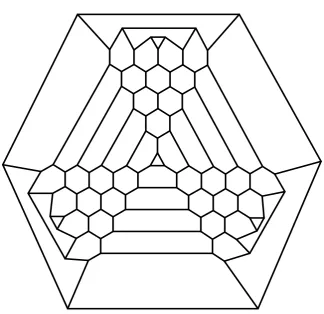
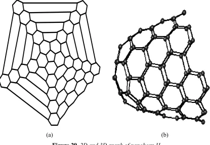
Carbon exists in several forms in nature. One is the so-called nanotube which

was discovered for the first time in 1991. Unlike carbon nanotubes, carbon nanohorns can be made simply without the use of a catalyst. The tips of these short nanotubes are capped with pentagonal faces; see Figure29. Let p, h, n and m be the number of pentagons, hexagons, carbon atoms and bonds between them, in a given nanohorn H. Then one can see that _{n r} 2_22r41,

2

3 65 112

2

r r

m   (r = 0,1,…) and the number of faces is f = p + h. By the Euler’s formula n − m + f = 2, one can deduce that

p = 5 and 2 21 24

2

r r

(a) (b)

Figure 29. 2D and 3D graph of nanohorn H.

In This paper by using definition of Omega polynomial we compute it for infinite class of nanohorn H depicted in Figure29.

Example 31. Consider the fullerene graph F24 in Figure 30. This fullerene graph has 36 edges. Similar to example 1 one can see that Ω(x) = 24x + 6x2 and so Sd(x)= 24x35 + 6x34. In Figure 30 one can see the planer graphs F24 and Le(F24).

Example 32. Consider the fullerene graph F26 depicted in Figure 31. This fullerene

graph has 39 edges. Similar to Examples 30 and 31 one can see that Ω(F26, x) = 21x + 9x2 and so, Sd(F24, x)= 21x38 + 9x37. By computing these polynomials for the Leapfrog fullerene we have:

Ω(x) = 24x3 _{+ 6x}6 _{+ x}9_.

2.4 POLYOMINO CHAINS OF 8–CYCLES

F24 Le(F24)

Figure 30. The leapfrog of graph F24.

F26 Le(F26)

Figure 31. The Leapfrog of graph F26.

Example 33. Consider the graph G shown in Figure 32. One can see this graph has

exactly 2 strips C1 and C2. On the other hand |C1| = 3 and |C2| = 2. Hence,

3 2

( ) 3x x 10x

   andSd x( ) 3 x2610x27.

e

e

Figure 33. The zig-zag chain of 8-cycles, n = 1.

Example 34. For the graph H depicted in Figures33, 34 there exist two distinct strips C1 and C2. Similarly, |C1| = 3 and |C2| = 2. Hence,

3 2

( ) 7x x 18x

   andSd x( ) 7 x28n218x28n1.

e

e

In generally, this graph has two distinct strips of lengths 2 and 3, respectively. In other words we have the following Theorem:

Theorem 35. Consider the graph of 2-polyomino system depicted in Figure 35. Then:

3 2

( ) (4x n 1)x (8n 2)x

     andSd x( ) (4 n1)x28n2(8n2)x28 1n. Consider now, another version of 2-polyomino system Hn. when n = 1, Figure

35, there exist three strips of length 2, 3 and 4, respectively. In other words,

4 3 2

( )x x 2x 13x

    andSd x( )x322x3313x34.

Similarly for n = 2 (Figure 36), there exist three strips of length 2, 3 and 4, respectively. This implies ( ) 2x  x45x324x2 and Sd x( ) 2 x675x6824x69.

By continuing this method it is easy to check that this graph has only three strips of length 2, 3 and 4, respectively. Thus by computing number of strips of equal size and substitute in the Omega polynomial the following Theorem can be deduced:

Theorem 36. Let Hn be the graph of 2-polyomino system shown in Figure 36. Then:

4 3 2

35 3 35 2 35 1

( ) (3 1) (11 2)

( ) n (3 1) n (11 2) n .

x nx n x n x and

Sd x nx  n x  n x 

     

    

e

_e

1

e

e₁ e₂

e₃

Figure 36. The graph of 2-polyomino system Hn, n = 2.

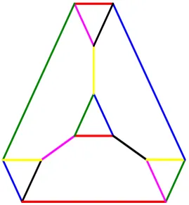
2.5 TRIANGULAR BENZENOID

In this section we compute counting polynomials mentioned in the text of triangular benzenoid graphs (see Figure 37). At first consider the graph of triangular benzenoid

G[n] for n = 1. The Omega and Sadhana polynomials are _{( ) 3x  x}2_{and ( ) 3x  x}4_, respectively. By continuing this method, there exist n strips of length 2, 3, …,n + 1, respectively. In other words, if C1, C2, …,Cn be all strips of G[n], then there are 3 strips

equivalent with |Ci|, i = 1, 2, …Hence we proved the following Theorem:

Theorem 37.

2 3 1

( [ ], ) 3(_{G n x x x x}n)

    _ and _{Sd G n x( [ ], ) 3( x}| | 2E _x| | 3E _{ x}| |E n 1₎

. . .

. .

. 1

2

3

n

Figure 37. The graph of triangular benzenoid graphs.

3.

PI

I

Let  be the class of finite graphs. A topological index is a function Top from  into real numbers with this property that Top(G) = Top(H), if G and H are isomorphic. Obviously, the number of vertices and the number of edges are topological index. The Wiener [46] index is the first reported distance based topological index and is defined as half sum of the distances between all the pairs of vertices in a molecular graph. If

, ( )

x y V G then the distance d x y_G( , )between x and y is defined as the length of any shortest path in G connecting x and y [47,48].

Khadikar introduced another index called Padmakar-Ivan (PI) index [49]. The PI index of a graph G is defined as:

PI = PI (G) = Σ [meu(e|G) + mev(e|G)]

where for edge e = uv, meu(e|G) is the number of edges of G lying closer to u than v, mev

(e|G) is the number of edges of G lying closer to v than u and summation goes over all edges of G. Similar to Sadhana polynomial we can define the PI polynomial. Then the PI index will be the first derivative of PI(x) evaluated at x=1.

Let Ce be a strips containing all parallel edges with e. If G be a bipartite graph it

is well – known fact that PI x( )



28 2 28 1

( ) 3(4 1) n 2(8 2) n .

PI x  n x   n x 

Theorem 39. Let Hn be the graph of 2-polyomino system shown in Figure 36. Then:

35 3 35 2 35 1

( ) 4 n 3(3 1) n 2(11 2) n .

PI x  nx   n x   n x 

Theorem 40. For the graph of triangular benzenoid graphs depicted in Figure 37 we

have:

| | 2 | | 3 | | 1

( [ ], ) 3(2 E 3 E ( 1) E n )

PI G n x  x   x   _ n x   .

where |E| = 28n + 1.

4.

O

I

C

N

Let G = (V,E) be a graph with finite vertex set V and edge set E (V ×V ) \ {(v, v) | vV

}. An edge (v,w) E is directed if ( , )w v E and undirected if (w, v) E. We denote a directed edge (v,w) by v → w and write v − w if (v,w) is undirected. If (v,w) E then v

and w are adjacent . If v → w then v is a parent of w, and if v − w then v is a neighbor of

w, see Figure 38.

A path in G is a sequence of distinct vertices <v0, …,vk> such that vi−1 and viare

adjacent for all 1 ≤i≤k. A path <v0, …,vk> is a semi-directed cycle if (vi, vi+1) Efor all 0 ≤i≤kand at least one of the edges is directed as vi→ vi+1. Here, vk+1≡v0. A chain graph is a graph without semi-directed cycles.

Let G G G ( ,...,₁ G v_k, ,..., )₁ v_k be a simple connected chain graph in Figure 39. Then

1

| ( ) | k | ( ) |_i

i

V G V G







1

| ( ) | ( 1) k | ( ) |_i

i

E G k E G



  



1

2

3

4

5

6

7

3

4 1

2

(a)

(b)

Figure 38. (a) Chain graph with chain components {1}, {2}, {3, 4} and {5, 6, 7};

....

G

₁

G

₂

G

k

Figure 39. Chain graph G G G ( ,...,1 G vk, ,..., ).1 vk

Lemma 41. Let G G G ( ,...,₁ G v_k, ,..., )₁ v_k be a simple connected chain graph and eE(G1) and f  E(G2). Then the edges e and f don’t satisfy in "co" relation. In the other words, e Θf .

Proof. Let e=ab  G1 and f = xyG2 be an arbitrary edges. We consider following case: (1) d a v( , )₁ d b v( , )₁ k₁andd x v( , )₂ d y v( , )₂ k₂ Then

1 1 2 2 1 2

( , ) ( , ) ( , ) ( , ) 1

d a y d a v d v v d v y   k k ,

1 1 2 2 1 2

( , ) ( , ) ( , ) ( , ) 1

d a x d a v d v v d v x   k k .

This implies that. eθ f .

(2) d a v( , )₁ d b v( , )₁ k₁ and d x v( , )₂ k d y v₂, ( , )₂ k₂1. So,

1 1 2 2 1 2

( , ) ( , ) ( , ) ( , ) 1

d a x d a v d v v d v x   k k and

1 1 2 2 1 2

( , ) ( , ) ( , ) ( , ) 1

d b x d b v d v v d v x   k k . This implies that e f eθ f .

(3) d a v( , )₁ k d b v₁, ( , )₁ k₁1 and so,

2 2 1 1 2 1

( , ) ( , ) ( , ) ( , ) 1

d x a d x v d v v d v a k  k and

2 2 1 1 2 1

( , ) ( , ) ( , ) ( , ) 1

d y a d y v d v v d v a k  k . This implies that. eθ f .

Lemma 42. Let G G G ( ,...,₁ G v_k, ,..., )₁ v_k be a chain graph and u V G ( )_i and v V G ( _j)

(1i j k i,  ,  j). So, d u v( , )d u v( , )i d v v( , )i j d v v( , )j d u v( , )i d v v( , ) 1j  .

Proof. We know d(ui,uj)=1 and this complete the proof.

Theorem 43. Let G be a simple connected graph with blocks G1, G2 and a cutedge uv,

u

v

G

_G

2

Figure 40. A graph G with a cutedge uv.

Proof. By using definition of omega polynomial and Lemma 1 one can see that

1 2

1 1 1 2 2 2 1 2

( , ) ( , ) c ( , ) c ( , ) ( , )

c c

G x x m G c x m G c x x G x G x

  





Corollary 44. If G G G ( ,...,₁ G v_k, ,..., )₁ v_k be a simple connected connected chain graph

then we have:

1

( , ) ( 1) ( , )

k

i i

G x k x G x



   



Theorem 45. Let G G G G v v ( ,_{1 2}, , )_{1 2} be simple connected chain graph. Then

1 2

( , )G x x ( , )G x ( , )G x

    ,

and

1 2

1 2

| ( )| | ( )| | ( )| 1

1 1 2 2

( , ) E G ( , ) E G c ( , ) E G c

c c

Sd G x _x  _





Corollary 46. Let G G G ( ,...,1 G vk, ,..., )1 vk so:

| ( )| | ( )| 1

1

( , ) ( 1) ( , ) i

i

k

E G c E G

i i c

i

Sd G x k x  m G c x 



  



1

( , ) ( 1) ( , )

k

i i

G x k x G x

 



  



Corollary 47. Let T be a tree with n vertices and T T_n T T( _n1, ,T v_{1 n1}, )v₁ .Thus we

have ( , ) (T xn  n1) .x

Proof. Let Tn-1 be a tree with n1 vertices constructed by cutting a vertex of degree 1 of

Tn. It is easy to see that ( , )T xn  (Tn1, )x x , (Tn1, )x  (Tn2, )x x and

2 1

( , )T x ( , )T x x

    . So, ( , ) (T x_n  n1) .x

Example 48. Consider graph of dendrimer D with n vertices, see Figure 41. Because

this graph is a tree with n vertices, we have ( , ) (D x  n1) .x

Theorem 49. Consider graph of nanostar dendrimer N with n vertices, see Figure 42. It

discussion in corollary 7 We have Gn G G( n1, ,G v1 n1, )v1 and then the following relations:

1 1

( , )G x_n x (G_n , )x ( , )G x

      ,

1 1

( , )G x_n (G_n, )x x ( , )G x

      ,

1 2 1

(Gn, )x (Gn , )x x ( , )G x

      ,

2 1 1

( , )G x ( , )G x x ( , )G x

      .

Now by summation of these relations we have

1 1

( , )G x_n ( , ) (G x n 1)x (n 1) ( , )G x

        . So ( , ) (G x_n  n1)x n G x ( , )₁ . But 2

1

( , ) 3G x x 9x

   . Thus, _{( , ) ( 1) (3 9 ) 9}2 2 _{(4 1)}

n

G x n x n x x nx n x

        ,

22 2 22 3

( , ) (4 1) n 9 n

n

Sd G x _ n_ x  _ nx  _{and ( , ) 18} 2 _{(4 1)}

n

G x nx n x

    .

Example 50.Suppose C20 denotes the fullerene graph on 20 vertices, see Figure 43(a). Then Ω(C20 , x) = 30x and so, Sd(C20,x) = 30x29.

Example 51. Suppose C30 denotes the fullerene graph on 30 vertices, see Figure 43(b). Then Ω(G, x) = 20x + 10x2 _{+ x}5 _{and so, Sd(G , x) = 20x}44 _{+ 10x}43 _{+ x}40_.

Example 52. Consider Table 3. In this table we compute the omega polynomial for

some fullerene graphs.

Theorem 53. Suppose Kn denotes the complete graph on n vertices. Then

( 1) ( , )

2

n n n

K x  x

  and so

( 3) 2 ( 1) ( , ) 2 n n

n n n

Sd K x x





 .

Proof. For every eE K( _n), C e( ) 1 and by using definition of omega polynomial the proof is trivial.

Theorem 54. Suppose T is a tree on n vertices. Then ( , ) T x  (n1)xand so,

2 ( , ) ( 1) n