VOLUME 40, ARTICLE 43, PAGES 1249
-
1290
PUBLISHED 15 May 2019
https://www.demographic-research.org/Volumes/Vol40/43/ DOI: 10.4054/DemRes.2019.40.43
Research Article
Taking birth year into account when analysing
effects of maternal age on child health and other
outcomes: The value of a multilevel-multiprocess
model compared to a sibling model
Øystein Kravdal
© 2019 Øystein Kravdal.
This open-access work is published under the terms of the Creative Commons Attribution 3.0 Germany (CC BY 3.0 DE), which permits use, reproduction, and distribution in any medium, provided the original author(s) and source are given credit.
1 Introduction 1250 1.1 Effects of maternal age on child health 1250 1.2 Controlling for selection through a sibling fixed-effects analysis 1251 1.3 The need to control for birth year, which is impossible in a sibling
analysis
1252
1.4 Multilevel-multiprocess models as a possible alternative 1254
1.5 Aims 1255
2 Data and methods 1257
2.1 Data source and cohorts 1257
2.2 Finding effects to be used in the simulation 1257
2.3 Simulating births and deaths 1259
2.4 Estimation of models from the simulated populations 1260
2.5 Number of replications 1261
2.6 Simulations with other assumptions 1262
3 Estimates from sibling models 1262
3.1 Estimation based on a simulated population where mortality was assumed to be unaffected by birth year
1263
3.2 Estimation based on simulated populations where a linear effect of birth year on mortality was assumed 1265
4 Estimates from multilevel-multiprocess models 1269
5 A reality that deviates from the standard assumptions of the multilevel-multiprocess model
1273
5.1 An additional variable correlated with the unobserved contributions to fertility and mortality
1273
5.2 An additional unobserved factor that is not normally distributed 1275
6 Summary and conclusion 1278
6.1 Sibling model 1278
6.2 The multilevel-multiprocess model as an alternative, but with some disadvantages
1279
6.3 The challenge in brief, and a suggested strategy 1280
7 Broadening the perspective 1282
8 Acknowledgements 1282
References 1283
Taking birth year into account when analysing effects of maternal
age on child health and other outcomes: The value of a
multilevel-multiprocess model compared to a sibling model
Øystein Kravdal1
Abstract
BACKGROUND
When analysing effects of maternal age on child outcomes, many researchers estimate sibling models to control for unobserved factors shared between siblings. Some have included birth year in these models, as it is linked to maternal age and may also have independent effects. However, this creates a linear-dependence problem.
OBJECTIVE
One aim is to illustrate how misleading the results may actually be when attempts are made to separate effects of maternal age and birth year in a sibling analysis. Another goal is to present and discuss the multilevel-multiprocess model as an alternative.
METHODS
Infant mortality was chosen as the outcome. Births and infant deaths were simulated from a multilevel-multiprocess model that included two equations for fertility, with a joint random effect, and one equation for infant mortality, with another random effect. The two random effects were set to be correlated. The effects of the independent variables were taken from simpler models estimated from register data. Various sibling models and multilevel-multiprocess models were estimated from these simulated births and deaths. In some simulations, two standard assumptions about the random effects were intentionally violated.
CONTRIBUTIONS
The paper illustrates how problematic it is to include both maternal age and birth year in a sibling model. Also, if only maternal age is included, but along with other reproductive variables, small categories should be used. It is argued that a multilevel-multiprocess model may be used instead to separate effects of maternal age and birth year, but this approach also has limitations, which are discussed.
1 Department of Economics, University of Oslo, and Centre for Fertility and Health, Norwegian Institute of
1. Introduction
1.1 Effects of maternal age on child health
There is a large literature on how maternal age is linked to child health, and the pattern is rather complex. On the one hand, studies have shown high child mortality and other adverse health outcomes at a low age among children whose mother was young when they were born (Finlay, Özaltin, and Canning 2011), and long-term disadvantages for these children have also been suggested (Bjørngaard et al. 2015; McGrath et al. 2004). On the other hand, there also seem to be disadvantages for children with old mothers. For example, some studies have shown a particularly high chance of being born pre-term or with low birth weight (Jacobsson, Ladfors, and Milsom 2004), which in turn may have implications for long-term health, education, and labour market outcomes (Black, Devereux, and Salvanes 2007). Furthermore, the chance of chromosomal or congenital abnormalities increases as a woman approaches the end of her reproductive period (Yoon et al. 1996), and advanced maternal age has been linked to childhood cancer (Johnson et al. 2009), diabetes (Cardwell et al. 2009), and more rare conditions such as autism (Lee and Grath 2015) and bipolar disorders (Menezes et al. 2010). A recent study indicates adverse consequences of high maternal age even for adult all-cause mortality (Barclay and Myrskylä 2018).
The relationship between maternal age and offspring health partly reflects genetic mechanisms in the mother, as well as in the father, whose age is typically not very different (Lee and Grath 2015; Menezes et al. 2010; Johnson et al. 2009; Yoon et al. 1996). Other physiological pathways may also contribute. For example, adverse effects of early motherhood may occur partly as a result of a particularly heavy nutritional burden during pregnancy (from feto-maternal competition) and physiological immaturity (Chen et al. 2007; Gibbs et al. 2012), especially in poor settings. It has also been suggested that hormonal factors with implications for the intrauterine environment are involved (Park et al. 2008).
(Powell, Steelman, and Carini 2006). This resource advantage associated with late motherhood may contribute to the better cognitive development and academic achievements observed in some studies among children with relatively old mothers (Tearne 2015), and it may also influence the children’s health in the long term for other reasons.
1.2 Controlling for selection through a sibling fixed-effects analysis
In addition to being a result of mechanisms such as those just mentioned, statistical relationships between maternal (or paternal) age at birth and child health (or other child outcomes) reflect joint determinants. These include the parents’ economic resources, work situation, education (operating not only through economic factors), health, and lifestyle preferences, whether the grandparents are able to provide various types of support, and resources and political attitudes in the community (which have implications, for example, for access to day-care centres and health services). For most purposes, one would like to control for these joint determinants as well as possible. Some of them may be quite adequately measured in the available data, and can then be included in a regression model for child health. However, realistically there will always be many unmeasured (or in practice unmeasurable) confounders. Stated differently, other child health determinants exist apart from maternal age and other characteristics that are measured and included in the child health model, and these ignored determinants may be correlated with maternal age.
In a number of studies, this problem related to unmeasured potential confounders has been partly solved by estimating sibling models, which means that the health among siblings is compared. Such an approach at least controls for maternal, household, and environmental factors that are shared between siblings. In principle, the importance of parental age for child health may also be analysed by means of ‘instruments’, i.e., factors (such as certain family events or policy changes) that can reasonably be assumed to lead to a lower or higher maternal age at birth, while not otherwise having an influence on child health. However, it is often difficult to find factors satisfying this requirement.
There may be differences between siblings that are linked to, but not a result of, the differences in maternal age, and which therefore would be particularly interesting to control for. For example, there is an obvious association between maternal age and birth order: The sibling who was born when the mother was older is bound to have a higher birth order. If we want an estimate that we can use to predict the implications of postponing the birth of the next child, or the first child, we would need to control for that. Furthermore, the siblings may have been born after different birth intervals, and one may want to separate the effect of birth interval from those of maternal age and birth order.
1.3 The need to control for birth year, which is impossible in a sibling analysis
Another important relationship is that the sibling born when the mother was oldest necessarily was also born in a later calendar year. Thus, in the absence of a control for birth year, the estimated effect of maternal age will reflect the sum of the effect of birth year and a more or less ‘pure’ effect of maternal age (depending on how many other factors linked to maternal age and affecting child health that are controlled for). Birth year may have an independent effect on child health because of, for example, general improvements in maternal nutrition (in poor settings), pre-natal care, or medical treatment after birth. If the intention is to predict the implication of postponing the birth of the first or the next child, which is bound to result in a correspondingly later year of birth, knowledge about such a combined effect (based on this kind of analysis that at least controls for unobserved factors shared between siblings) may be sufficient. However, it could also be argued that it would be valuable to know the separate effects of maternal age and birth year and then base predictions on the sum of these. This is because, while the maternal age effect may well remain quite constant some time into the future (and perhaps especially the component that is produced by biological rather than social mechanisms), there may be more doubt about the persistence of the birth-year effect. There may be good reasons both to assume that the future effect will not be as strong as in the past and to assume the opposite, and by allowing the summation of effects people are free to make their own assumptions. Additionally, obtaining effects that are as ‘pure’ as possible is typically a goal from a scientific perspective. For example, the aim may be to learn about bio-medical processes linked to maternal age, and then the contribution from the birth-year effect (and as many as possible of the social effects) definitely has to be wiped out.
child’s educational career because of increasing pressure to take post-secondary education or larger economic support to do so (Breen 2010).
The recent register-based analysis of four social and health effects of maternal age by Barclay and Myrskyla (2016) is one example of an investigation aiming to separate out the birth-year effect. Another is the study by Bjørngaard et al. (2015), who add a crude control for birth year when estimating the importance of maternal age for offspring suicide risks. Kudamatsu (2012) and Molitoris (2018) include both maternal age and birth year in their studies of infant mortality, but without paying much attention to the effects of these two variables, as their focus is on other mortality determinants.
However, it is not possible to separate the effects of maternal age and birth year in a sibling analysis without making some bold assumptions. As explained very well by Keiding and Andersen (2016), this is because the child’s birth year (B) minus the mother’s age at the child’s birth (A) is the mother’s birth year (MB), which is the same for all siblings and can be considered part of the sibling fixed effect. Thus, we are faced with a linear-dependence problem often referred to by demographers as an age-period-cohort problem. Regardless of how the effects of A and B are specified – they may, for example, be included as grouped variables – the model is indistinguishable from a model where a linear trend is added to the effect of A and subtracted from the effect of B. Of course, effects can be estimated if assumptions are made about one of the linear components, but typically there is no theoretical basis for making such assumptions.
To illustrate the problem mathematically in a very simple way with linear effects of maternal age and birth year, assume that a certain continuous health outcome Yij for
child i in sibling group j is given by
Yij = b0 +b1Aij + b2 Bij +ej+ εij, (1)
where ej (sibling fixed effect) is an addition to Yij that is shared by the siblings and εij is
a child-specific error term. In a sibling analysis where there are only two siblings (to further simplify the example), essentially the following equation is estimated, which involves differences in Y, A, and B between the siblings:
∆Yj = b1∆Aj + b2∆Bj + ∆εj.
Since ∆Aj = ∆Bj, the right hand side can alternatively be written as (b1+b2) ∆Aj or
(b1+b2) ∆Bj. Thus, either A or B can be included, and in both cases the estimated effect
is the sum b1+b2 of the true effects: there is no way to find out how large b1 and b2 are.
models, readers should be warned (as in Barclay and Myrskylä 2018) that there is much uncertainty about the corresponding separate effects.
1.4 Multilevel-multiprocess models as a possible alternative
As should be clear by now, the idea behind the sibling model is to add sibling fixed effects (ej in Equation 1) to control for unobserved characteristics shared by siblings
that may affect their health, and that may also be correlated with maternal age (A in Equation 1), other reproductive factors, or other types of variables included in the model. Is there another way to take into account unobserved determinants of child health that are shared by siblings, and that are somehow linked to the reproductive factors? One possibility might be to explicitly model the link between the unobserved health determinants and the reproductive factors using random effects, and it would make good sense to do that by considering the birth rates as the ‘building blocks’ behind the reproductive factors. More concretely, a model might be specified that includes equations for parity transitions and child health, and in which there are some observed determinants (including reproductive factors in the health equation) plus mother-specific fertility and health random effects that represent effects of unobserved characteristics of the mother (and her household and the environment where she lives), and that are correlated with each other. A simple version of this would be to include one constant health random effect, reflecting that the health of all siblings is influenced by the unobserved factors in the same way, as well as one constant fertility random effect, reflecting that there is a similar contribution from the unobserved factors for all parity transitions. Such models are often referred to as multilevel-multiprocess models (the highest ‘level’ being the mother, and the second and lowest level the children or the mother’s different parity transitions, while the ‘processes’ are fertility and child health). It is typically assumed when estimating such models that the random effects are normally distributed and uncorrelated with the observed variables (except that the health random effect in this case obviously would be correlated with the reproductive factors in the health equation, because the latter are realizations of a model including a fertility random effect that is correlated with the health random effect). Multilevel-multiprocess models of this type are central to this paper, but other versions of multilevel-multiprocess models will also receive some attention.
model, women with only one child also contribute to the estimation, although not in the estimation of the distribution of the random effects.
Identification of a multilevel-multiprocess model of the type specified here requires that there are at least some individuals for whom there are at least two observations or ‘spells’ in each ‘process’. This requirement is obviously satisfied in this case, since many women have more than one child. (See Steele, Sigle-Rushton, and Kravdal 2009, Väisänen 2017, and Kravdal 2018 for examples of how multilevel-multiprocess models have been used in demographic research recently.)
1.5 Aims
One goal of this paper is to illustrate how misleading the results can be when birth year is added in a sibling fixed-effects analysis of effects of maternal age, by means of a simulation experiment where infant mortality (rather than another indicator of child health) is the outcome. Although the problem is obvious mathematically and well known to many researchers, it may be useful to see some examples of its importance in practice. The reason for using a simulation-based approach is that if the simulated population satisfies the assumptions of the model and large or many replications are made, a good estimation procedure should produce effect estimates close to the corresponding effects used in the simulation (the ‘true’ effects). The other goal, also involving simulation, is to discuss the value of a multilevel-multiprocess model as an alternative to the sibling model.
More specifically, the first step of the analysis (presented in Section 2) is to simulate populations with characteristics or behaviours that are handled well by the sibling model, i.e., constant unobserved mortality determinants somehow link to the reproductive factors. This is done by simulating from a multiprocess-multilevel model, just as described in the preceding sub-section. A link is established between the unobserved mortality determinants and the reproductive factors in the mortality equation by drawing constant mother-specific contributions to fertility and mortality (random effects) from a bivariate normal distribution with a certain correlation, chosen arbitrarily. The reproductive factors are birth order and birth interval length in addition to maternal age. As already indicated, these are closely related to maternal age, and they have attracted much attention in the literature on how reproductive factors affect child health, mortality, and well-being (Barclay and Kolk 2017; Black, Devereux, and Salvanes 2005; Kravdal 2018). Birth year is also included in the mortality equation in most of the simulations.
that is unimportant. If sibling models with birth year included were to give very ‘wrong’ estimates using these particular simulated populations, that would be sufficient ground for general concern about this kind of estimation. However, simulation based on other assumptions is carried out in the last part of the analysis, as explained below.
In the second step, sibling models are estimated from the simulated populations, and the resulting effects are compared with those used in the simulation (Section 3). The third step shows that the effects of the different reproductive variables and birth year (and other variables) can be correctly estimated from the simulated populations using a multilevel-multiprocess model, specified just as the one used in the simulation (Section 4). While this might be considered a trivial circularity it confirms that the estimation and simulation procedures are working as they are supposed to, and hopefully strengthens confidence in all parts of the analysis. Also, this check is supplemented by estimations that illustrate how sensitive the results are to the categorization of maternal age. The categorization of maternal age is a potential concern because of the close relationship between this variable and the other reproductive variables. For comparison, it is also shown how important it may be to use a finely specified maternal-age variable when estimating sibling models.
2. Data and methods
2.1 Data source and cohorts
The effects used in the simulation were derived from the effects in quite simple fertility and mortality equations (specified below), estimated from Norwegian register data for the years up to 2008 for women born in Norway in 1950–1964 and still living in the country when they were 44 years old. For data protection purposes there was only information about their children’s year of birth, not month of birth. Women who bore two or more children in the same year, most of whom were probably twins, were excluded from the estimation.
2.2 Finding effects to be used in the simulation
The first step was to estimate the following discrete-time hazard models for first and higher-order births, up to the fifth, between age 17 and maximum age 44:
log (p(1)/(1–p(1))) = β(1)
0 +β(1)1A +β(1)2Y +β(1)3E +β(1)4AE +β(1)5(year-1980)A,
and
log (p(2)/(1–p(2))) = β(2)
0 +β(2)1A +β(2)2Y +β(2)3E +β(2)4D+β(2)5F.
p(1) is the probability of having a first child during the calendar year, while p(2) is
the probability of having a nth child during the calendar year given that the mother’s
parity at the beginning of the year was n–1, and n is two or higher. The superscripts(1)
and(2) are used similarly for other variables.A is a vector of dummies corresponding to
later education (Cohen, Kravdal, and Keilman 2011). If the goal is to learn something about causal effects of education on fertility, a measure of current education rather than education at age 44 should be included. However, full education histories were not available for these cohorts, and because the intention is only to discuss the value of certain methods, the inclusion of education at age 44 should be of no concern.
In addition to a weak general decline in first-birth rates, and thus slight increase in the proportion remaining childless, there has been a shift towards later entry into parenthood: First-birth rates have fallen most sharply at the lowest ages and have increased among the oldest women. For simplicity, this change in the age pattern was specified as a linear interaction between period (minus 1980) and each of the age dummies.D is a vector of dummies for duration since last previous birth, corresponding to 1, 2, 3 (reference), 4, 5–6, 7–9, and 10 or more years.F is a vector of dummies for the number of children already born, which is 1 (reference), 2, 3, or 4. The observations were censored at the time of fifth birth or at age 44, whichever came first (recall that only those alive up to age 44 were included and that the last year of observation, 2008, was at age 44 or later). The βs are the corresponding effects.
Also, the following model for the chance (m) of dying within the calendar year after the year of birth was estimated (for each of the children included in the fertility analysis except those born in 2008, as they were not observed through the subsequent year):
log (m/(1–m)) = γ0 +γ1A+ γ2B +γ3E +γ4D+γ 5O.
The vectorsA,D, andE are as just defined (i.e.,A represents maternal age at the end of the year when the child was born andD represents the length of the previous birth interval). The D-dummies are set to 0 for first-born children. O represents the child’s birth order, which is mother’s parity at the beginning of the year when the child is born (represented byF in the fertility equation) plus 1. Theγs are the corresponding effects. B is the birth year, and for simplicity a linear birth-year effect is assumed.
2.3 Simulating births and deaths
Half of the women included in the fertility and mortality estimation (224,927 women) were randomly selected and used as the basis population in all simulations. In total, up to 100 simulations of a certain type were carried out for this basis population, each of them creating what is referred to below as a ‘simulated population’ (see sub-section 2.5 on the number of replications). This population size was chosen because it was close to the maximum that could be handled in the estimation of the multilevel-multiprocess models with the chosen software (see details below). For each of the women, the simulation of births and infant deaths was based on the values of the cohort and education variables, the estimates of the βs in the fertility equation, and a slightly modified version of the estimates of the γs in the mortality equation. Let us call these two sets of effects β^ and γ^.
The estimated maternal-age effects in the mortality equation were modified in two steps. First, effects for all maternal ages 17–44 in one-year categories were defined by setting the effects for age 18, 21, 24, etc., equal to the effects estimated for the corresponding three-year age groups (17–19, 20–22, 23–25, etc.), and then interpolating and extrapolating. This was done because, in reality, infant mortality is not a step-function of maternal age, and it is particularly important to make realistic assumptions about the effects of that variable. Second, some irregularities (partly reflecting the small number of observations in some categories) were smoothed out, because the effects used in the simulation of mortality are shown in tables and compared with results obtained when various models are estimated from the simulated population, and such comparison is simpler when the effects are smoother. Additionally, the effects of interval and birth order were smoothed, and the effect of birth year was set to be somewhat stronger than the one that was estimated.
Furthermore, one random effect (called δ) was added to the two fertility equations and another random effect (called ε) to the mortality equation when simulating. The former represents constant unobserved factors affecting the woman’s fertility throughout her reproductive career, and the latter represents constant unobserved factors affecting the mortality of all her children. Both random effects were assumed to be normally distributed with mean 0 and standard deviation 1 (any other number could have been chosen), and the correlation between them was set arbitrarily to 0.5, which can be considered a quite strong correlation. In other words, for each woman in the simulated population, two numbers were drawn (at age 17 when the simulation starts) from a bivariate normal distribution with the mentioned means, standard deviations, and correlation. Thus, the equations used in the simulation were as follows:
log (p(1)/(1–p(1))) = β^ (1)
0 +β^(1)1A +β^(1)2Y +β^(1)3E +β^(1)4AE
+β^(1)
log (p(2)/(1–p(2))) = β^ (2)
0 +β^(2)1A+β^(2)2Y +β^(2)3E +β^(2)4D+β^(2)5F + δ
log (m/(1–m)) = γ^0 +γ^1*A*+γ^2B +γ^3E +γ^4D+γ^5O+ ε. (2)
The maternal age variable and the corresponding effects in the mortality equation are now marked with * to symbolize the change to one-year categories.
One-year steps were taken in the simulation: For each year of the woman’s life between age 17 and 44 her probabilities of having a child that year and losing the child within the subsequent year were predicted. A childbirth, and possibly a death of that child, was ‘assigned to’ the woman in that year depending on whether two numbers drawn from uniform distributions over [0,1] were lower than the respective predicted probabilities. (The fact that, for simplicity, a death was assigned in the same year as the birth has no implications for the later estimation, where the outcome is considered as death within the year of birth or the subsequent year.)
Birth year was left out of the mortality equation in some introductory simulations, to set up a contrast to the later and main simulations. In another introductory simulation the two random effects were omitted. In the latter case, the simulated number of births in the different cohorts, the average age at first birth, and the variation in these figures across educational categories accorded very well with findings reported elsewhere (e.g., Kravdal and Rindfuss 2008). This indicates that the estimation of fertility models in the first step and the fertility part of the simulation was done correctly.
2.4 Estimation of models from the simulated populations
The multilevel-multiprocess models that were estimated were specified exactly as model (2) in the simulation, except that it was experimented with some alternative categorizations ofA.A few different categorizations ofAwere also used in the sibling models, and in some of them birth year was included as a categorical variable, or even left out. All this is specified in detail below.
The estimation of sibling models was carried out with SAS software, as was the simulation, the estimation of effects to be used in the simulation, and the construction of data (from the simulated populations) to be used as input to estimate the multilevel-multiprocess models. The latter estimation was done with the aML software (Lillard and Panis 2003). Other software also exists for such purposes. In particular, there are modules in Stata (Bartus and Rodman 2014) or MLwiN (see an example by Väisänen 2017) that may be used.
it was sufficient to use 20 support points. Using 30 support points gave exactly the same estimates, and (as described below) the estimates (averaged over several replications) from a multilevel model that corresponded exactly to the one used in the simulation were almost identical to the true effects when 20 support points were used. The typical CPU-time for the estimation of one multilevel-multiprocess model from a simulated population was about 1 hour. As mentioned, the simulated population could not be much larger (given the number of variables considered). If it were about 20% larger, estimation would be impossible because of insufficient computer memory. (Recall, however, that the simulated population included as many as 224,927 women, and therefore would be considered large by most standards.)
2.5 Number of replications
Most of the analysis was based on 100 simulated populations of the size just mentioned. Models were estimated from all these, after which the average over the 100 sets of estimates was calculated. This procedure was quite cumbersome when multilevel-multiprocess models were estimated, because of the switching between two types of software (SAS and aML), the long CPU-time, and the large data sets used in the estimation, and it was necessary to break the process into five rounds with 20 simulated populations. Fortunately, the results were very similar when 10 simulated populations were used instead – reflecting the large size of these populations. For simplicity, the last part of the analysis involving multilevel-multiprocess models was therefore based on only 10 simulated populations.2
2 Note that this simulation-estimation experiment might have been based on simpler fertility equations in the
2.6 Simulations with other assumptions
In a final step, alternative simulations were carried out where it was no longer assumed that random effects were normally distributed and uncorrelated with the observed factors, in order to see how wrong the estimates from a multilevel-multiprocess model (still with standard assumptions about the random effects) would then be. In some of these alternative simulations, a variable G was added:
log (p(1)/(1–p(1))) = β^ (1)
0 +β^(1)1A +β^(1)2Y +β^(1)3E +β^(1)4AE
+β^(1)
5(year-1980)A +β(1)6G +δ
log (p(2)/(1–p(2))) = β^ (2)
0 +β^(2)1A+β^(2)2Y +β^(2)3E +β^(2)4D+β^(2)5F +β(2)
6G + δ
log (m/(1–m)) = γ^0 +γ^1*A*+γ^2B +γ^3E +γ^4D+γ^5O +γ6G + ε. (3)
G was a number drawn randomly for each woman from a standard normal distribution and made to correlate with ε, and thus δ. Other simulations instead included H or K, which were defined as 1 if G was larger than 0 or 0.67, respectively, and 0 otherwise. In one set of estimations of multilevel-multiprocess models, G, H, or K were included in the models to examine the implications of having an observed determinant of fertility and mortality (with one of three different distributions) that was correlated with the unobserved normally distributed contributions to mortality and fertility (i.e., ε
and δ). In another set of estimations, H and K were not included in the models, but were instead considered as adding to the unobserved contributions to mortality and fertility, which were then no longer normally distributed. H and K did not have to be correlated with ε and δ in this illustration of the implications of deviations from normality; it was just convenient to use the same variables in this part of the analysis. In a supplementary step a version of H that was uncorrelated with ε and δ was used instead, and this gave very similar results. See further description of these simulation-estimation experiments below.
3. Estimates from sibling models
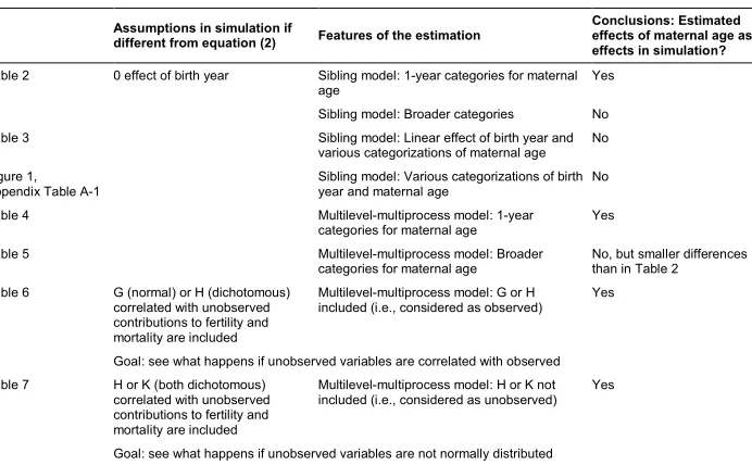
Table 1: Overview of simulations, estimations, and results
Assumptions in simulation if
different from equation (2) Features of the estimation
Conclusions: Estimated effects of maternal age as effects in simulation?
Table 2 0 effect of birth year Sibling model: 1-year categories for maternal
age Yes
Sibling model: Broader categories No
Table 3 Sibling model: Linear effect of birth year and various categorizations of maternal age No Figure 1,
Appendix Table A-1
Sibling model: Various categorizations of birth year and maternal age
No
Table 4 Multilevel-multiprocess model: 1-year
categories for maternal age Yes
Table 5 Multilevel-multiprocess model: Broader
categories for maternal age No, but smaller differencesthan in Table 2 Table 6 G (normal) or H (dichotomous)
correlated with unobserved contributions to fertility and mortality are included
Multilevel-multiprocess model: G or H included (i.e., considered as observed)
Yes
Goal: see what happens if unobserved variables are correlated with observed Table 7 H or K (both dichotomous)
correlated with unobserved contributions to fertility and mortality are included
Multilevel-multiprocess model: H or K not included (i.e., considered as unobserved)
Yes
Goal: see what happens if unobserved variables are not normally distributed
3.1 Estimation based on a simulated population where mortality was assumed to be unaffected by birth year
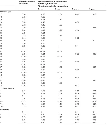
Table 2: Averages of effects on infant mortality estimated from 100 simulated populations, when the effect of birth year is set to 0 in the simulations
Effects used in the
simulationa Estimated effects in sibling fixed-effects logistic modelb Size of categories for maternal age
1 year 2 years 3 years 5 years Maternal age
17 0.66 0.66 0.54 0.42 0.23
18 0.60 0.60
19 0.54 0.54 0.43
20 0.48 0.48 0.30
21 0.42 0.42 0.33
22 0.36 0.36 0.09
23 0.30 0.30 0.23 0.16
24 0.24 0.24
25 0.18 0.18 0.12
26 0.13 0.13 0.05
27 0.09 0.09 0.05 0
28 0.05 0.05
29 0.02 0.02 0 0
30 0 0
31 ‒0.02 ‒0.02 ‒0.02
32 ‒0.04 ‒0.04 ‒0.03 0.00
33 ‒0.06 ‒0.06 ‒0.06
34 ‒0.08 ‒0.08
35 ‒0.08 ‒0.08 ‒0.07 ‒0.03
36 ‒0.08 ‒0.08
37 ‒0.08 ‒0.09 ‒0.07 0.05
38 ‒0.08 ‒0.08 0.00
39 ‒0.08 ‒0.09 ‒0.05
40 ‒0.08 ‒0.07
41 ‒0.08 ‒0.09 ‒0.06 0.00
42 ‒0.08 ‒0.10 0.08
43 ‒0.08 ‒0.09 ‒0.06
44 ‒0.08 ‒0.09 0.01
Previous interval
1 0.57 0.58 0.58 0.59 0.61
2 0.07 0.07 0.08 0.08 0.09
3 0 0 0 0 0
4 ‒0.05 ‒0.05 ‒0.05 ‒0.06 ‒0.07
5‒6 ‒0.12 ‒0.12 ‒0.13 ‒0.14 ‒0.16
7‒9 ‒0.12 ‒0.12 ‒0.14 ‒0.17 ‒0.20
10+ ‒0.12 ‒0.12 ‒0.16 ‒0.21 ‒0.29
Birth order
1 0 0 0 0 0
2 0.10 0.10 0.08 0.05 0.00
3 0.20 0.20 0.16 0.11 0.02
4 0.30 0.30 0.24 0.17 0.05
5 0.40 0.40 0.33 0.23 0.09
Notes:a The model used in the simulation was as explained in the text. The effect of birth year on infant mortality was assumed to be
0.b The model included the variables shown in this table plus sibling fixed effects. The estimates that are shown for age x are for a
When two-year categories for maternal age were used (Table 2, column 3) the effects of maternal age and birth order were about 20% weaker (judging by the difference in mortality between the lowest and highest age group) than when one-year categories were used. Further changes in the same direction occurred when the maternal-age categories were increased to three or five years (Table 2, columns 4 and 5). In fact, when five-year categories were used, the estimated effects of maternal age and birth order were about 80% weaker than the corresponding true values. The effects of the birth interval length became stronger as the effects of birth order and maternal age became weaker.
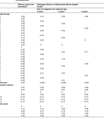
3.2 Estimation based on simulated populations where a linear effect of birth year on mortality was assumed
When a linear effect of birth year was included in the mortality equation in the simulation, the estimates from sibling models (now including birth year) were no longer close to the true values, even when small categories for maternal age were used.
Table 3: Averages of effects on infant mortality estimated from 100 simulated populations, using different categorizations of maternal age in the estimation
Effects used in the
simulationa Estimated effects in sibling fixed-effects logisticmodelb Size of categories for maternal age
2 years 3 years 5 years Maternal age
17 0.66 0.10 0.06 0.06
18 0.60
19 0.54 0.07
20 0.48 0.02
21 0.42 0.03
22 0.36 0.00
23 0.30 0.00 ‒0.02
24 0.24
25 0.18 ‒0.03
26 0.13 ‒0.04
27 0.09 ‒0.03 0
28 0.05
29 0.02 0 0
30 0
31 ‒0.02 0.05
32 ‒0.04 0.07 0.11
33 ‒0.06 0.09
34 ‒0.08
35 ‒0.08 0.16 0.18
36 ‒0.08
37 ‒0.08 0.24 0.29
38 ‒0.08 0.32
39 ‒0.08 0.35
40 ‒0.08
41 ‒0.08 0.41 0.43
42 ‒0.08 0.47
43 ‒0.08 0.50
44 ‒0.08 0.51
Birth year ‒0.02 ‒0.063 ‒0.063 ‒0.061
Previous interval
1 0.57 0.58 0.58 0.58
2 0.07 0.07 0.07 0.08
3 0 0 0 0
4 ‒0.05 ‒0.05 ‒0.05 ‒0.05
5‒6 ‒0.12 ‒0.12 ‒0.12 ‒0.12
7‒9 ‒0.12 ‒0.12 ‒0.12 ‒0.12
10+ ‒0.12 ‒0.12 ‒0.12 ‒0.13
Birth order
1 0 0 0 0
2 0.10 0.10 0.09 0.08
3 0.20 0.19 0.19 0.16
4 0.30 0.30 0.29 0.26
5 0.40 0.40 0.39 0.35
Notes:a The model used in the simulation was as explained in the text.b The model included the variables shown in this table plus
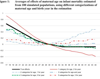
In the second set-up, birth year was included in the regression models as a categorical variable, and a few different categorizations were tried. One-year categories cannot be specified for both maternal age and birth year, but various other combinations of one-, two-, three-, and five-year categories were experimented with. When one-year categories were specified for maternal age and two-year categories were specified for birth year, very sharp effects of maternal age appeared, while there was essentially no effect of birth year (see plots of maternal age effects in Figure 1; effects of all variables are shown in Table A-1). In the opposite situation, with two-year categories for maternal age and one-year categories for birth year, the effect of maternal age was positive, while there was a strongly negative effect of birth year. The estimates were closer to the true values when using two-year categories for both maternal age and birth year, although – most importantly – the estimated negative effect of maternal age was too weak (only about 60% of the true effect). The effect of birth year was too strongly negative compared to the true value of –0.02 per year, which corresponds to –0.82 over the 41-year period. A similar pattern appeared when three-year categories were used for both maternal age and birth year (not shown in figure or table).
Figure 1: Averages of effects of maternal age on infant mortality estimated from 100 simulated populations, using different categorizations of maternal age and birth year in the estimation
-0.6 -0.4 -0.2 0 0.2 0.4 0.6 0.8 1
17 18 19 20 21 22 23 24 25 26 27 28 29 30 31 32 33 34 35 36 37 38 39 40 41 42 43 44
When three-year categories were used for maternal age and five-year categories were used for birth year the effect of maternal age was again too weakly negative, but the deviation from the true effect was smaller than with the other specifications (the difference in mortality between the lowest and highest age being about 20% smaller than the corresponding true values). With this specification the effect of birth year was also too weak, and the effect of birth order was strongly underestimated. Using instead five-year categories for maternal age and three-year categories for birth year, a U-shaped effect of maternal age appeared, while the effect of birth order became smaller than in any of the other models, and the effect of birth year again became too negative.
Note that the differences in results across various categorizations of maternal age do not just reflect the problem related to separation of effects of the reproductive variables that appeared when birth year was kept out of the simulation and estimation (shown in Table 2). Patterns similar to those shown in Figure 1 and Table A-1 were also found when birth order and birth interval were excluded from the simulation and estimation (not shown in tables). In this alternative set-up, the estimates obtained with three-year categories for maternal age and five-year categories for birth year were still those that came closest to the true values, and they were now actually even closer. With the other categorizations, effects of maternal age remained almost unchanged when birth order and birth interval effects were excluded, while birth year effects became more strongly negative.
4. Estimates from multilevel-multiprocess models
Estimates from multilevel-multiprocess models are shown in Table 4. They are very close to the true values, regardless of whether 10 or 100 replications are used, which, as mentioned, justifies the use of 10 replications in the remaining analysis.
Table 4: Averages of effects on infant mortality estimated from 10 or 100 simulated populations, using a multilevel-multiprocess model in the estimation
Effects used in simulationa Estimates from multilevel‒ multiprocess modelb Average over 10 simulated
populations Average over 100 simulatedpopulations Maternal age
17 0.66 0.67 0.66
18 0.60 0.59 0.61
19 0.54 0.55 0.54
20 0.48 0.48 0.48
21 0.42 0.42 0.42
22 0.36 0.38 0.36
23 0.30 0.30 0.30
24 0.24 0.25 0.24
25 0.18 0.19 0.18
26 0.13 0.13 0.13
27 0.09 0.11 0.09
28 0.05 0.05 0.05
29 0.02 0.02 0.02
30 0 0 0
31 ‒0.02 ‒0.01 ‒0.02
32 ‒0.04 ‒0.02 ‒0.04
33 ‒0.06 ‒0.06 ‒0.06
34 ‒0.08 ‒0.06 ‒0.08
35 ‒0.08 ‒0.08 ‒0.09
36 ‒0.08 ‒0.07 ‒0.08
37 ‒0.08 ‒0.04 ‒0.08
38 ‒0.08 ‒0.05 ‒0.08
39 ‒0.08 ‒0.05 ‒0.07
40 ‒0.08 ‒0.07 ‒0.07
41 ‒0.08 ‒0.08 ‒0.09
42 ‒0.08 ‒0.07 ‒0.11
43 ‒0.08 ‒0.09 ‒0.09
44 ‒0.08 ‒0.07 ‒0.10
Birth year ‒0.02 ‒0.020 ‒0.020
Previous interval
1 0.57 0.57 0.57
2 0.07 0.06 0.07
3 0 0 0
4 ‒0.05 ‒0.06 ‒0.05
5‒6 ‒0.12 ‒0.12 ‒0.12
7‒9 ‒0.12 ‒0.13 ‒0.12
Table 4: (Continued)
Effects used in simulationa Estimates from multilevel‒ multiprocess modelb Average over 10 simulated
populations Average over 100 simulatedpopulations Birth order
1 0 0 0
2 0.10 0.11 0.10
3 0.20 0.20 0.20
4 0.30 0.30 0.30
5 0.40 0.39 0.40
Education
10 0 0 0
11 ‒0.08 ‒0.09 ‒0.08
12‒13 ‒0.16 ‒0.17 ‒0.16
14+ ‒0.24 ‒0.25 ‒0.24
Std. fertility random term 1.0 1.00 1.00
Std. mortality random
term 1.0 1.00 1.00
Corr. random terms 0.5 0.51 0.50
Notes:a The model used in the simulation was as explained in the text.b The equation for mortality included the variables shown in
this table, and there were also equations for fertility, as explained in the text.
Table 5: Averages of effects on infant mortality estimated from 10 simulated populations, using a multilevel-multiprocess model in the estimation and different categorizations of maternal age
Effects used in
simulationa Estimated effects in multilevelmodelsb ‒multiprocess Size of categories for maternal age
2 years 3 years 5 years Maternal age
17 0.66 0.59 0.53 0.35
18 0.60
19 0.54 0.46
20 0.48 0.37
21 0.42 0.36
22 0.36 0.14
23 0.30 0.24 0.21
24 0.24
25 0.18 0.13
26 0.13 0.08
27 0.09 0.06 0
28 0.05
29 0.02 0 0
30 0
31 ‒0.02 ‒0.05
32 ‒0.04 ‒0.04 ‒0.05
33 ‒0.06 ‒0.07
34 ‒0.08
35 ‒0.08 ‒0.09 ‒0.06
36 ‒0.08
37 ‒0.08 ‒0.08 ‒0.02
38 ‒0.08 ‒0.03
39 ‒0.08 ‒0.07
40 ‒0.08
41 ‒0.08 ‒0.11 ‒0.08
42 ‒0.08 ‒0.02
43 ‒0.08 ‒0.14
44 ‒0.08 ‒0.08
Birth year ‒0.02 ‒0.021 ‒0.022 ‒0.026
Previous interval
1 0.57 0.57 0.57 0.58
2 0.07 0.07 0.07 0.08
3 0 0 0 0
4 ‒0.05 ‒0.05 ‒0.05 ‒0.05
5‒6 ‒0.12 ‒0.13 ‒0.14 ‒0.14
7‒9 ‒0.12 ‒0.12 ‒0.13 ‒0.13
Table 5: (Continued)
Effects used in
simulationa Estimated effects in multilevelmodelsb ‒multiprocess Size of categories for maternal age
2 years 3 years 5 years Birth order
1 0 0 0 0
2 0.10 0.10 0.09 0.06
3 0.20 0.19 0.18 0.13
4 0.30 0.29 0.26 0.20
5 0.40 0.39 0.36 0.28
Education
10 0 0 0 0
11 ‒0.08 ‒0.08 ‒0.08 ‒0.10
12‒13 ‒0.16 ‒0.16 ‒0.17 ‒0.18
14+ ‒0.24 ‒0.24 ‒0.24 ‒0.27
Std. fertility random
term 1.0 1.00 1.00 1.00
Std. mortality random
term 1.0 1.00 1.00 1.01
Corr. random terms 0.5 0.51 0.51 0.53
Notes:a The model used in the simulation was as explained in the text.b The equation for mortality included the variables shown in
this table, and there were also equations for fertility, as explained in the text. The estimates that are shown for age x are for a category including ages x to x+1 (second column), x+2 (third column), or x+4 (fourth column), except that the highest age category only includes ages up to 44.
If birth year was not included in the mortality equation in the multilevel-multiprocess model, the estimated effect of maternal age (difference between mortality in lowest and highest age) was almost the same as the true effect of maternal age plus 27 times the effect of birth year (not shown in tables). In other words – and as expected – the birth year effect was captured by the maternal-age effect, just as with the sibling analysis.3
3 Note that because some combinations of maternal age and birth order are impossible or very rare, the use of
5. A reality that deviates from the standard assumptions of the
multilevel-multiprocess model
So far, it has been assumed in the simulations that the random effects, which reflect unobserved constant mother-level contributions to mortality and fertility, are normally distributed and uncorrelated with the observed variables (except that the unobserved contribution to mortality is correlated with the mortality determinants that are a result of fertility because of the correlation between the unobserved contributions to fertility and mortality). These assumptions were also built into the estimation of multilevel-multiprocess models presented in the foregoing section. How would the estimation of such models go if these two assumptions fit poorly with reality? Examples of this are given below by carrying out alternative simulations with other assumptions about the random effects, and then estimating the models similar to those above.
5.1 An additional variable correlated with the unobserved contributions to fertility and mortality
The first step was to create a population where the normally distributed unobserved contributions to fertility and mortality are correlated with a variable considered as an observed determinant. This was done by adding a standard normally distributed variable G that was strongly related to the mortality random effect (correlation 0.70) – and therefore also to the fertility random effect – to both the mortality and fertility equations in the simulation, as shown in (3). G was considered as an observed variable and assumed to have large effects: The coefficients β(1)6 and β(2)6 in the two fertility
equations were arbitrarily set to 1.1 (i.e., the log-odds of having a child is 1.1 higher when G = 1 than when G = 0), and the coefficient γ6 in the mortality equation was set to
0.8.
uncorrelated with G. The latter may be considered as represented by the mortality random effect in the model that is estimated.
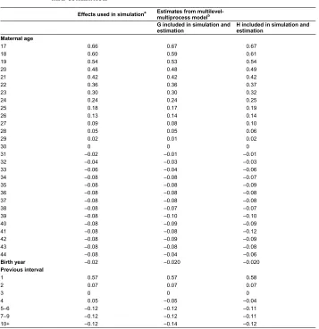
Table 6: Averages of effects on infant mortality estimated from 10 simulated populations, using a multilevel-multiprocess model, and when a variable (G or H) that is correlated with the unobserved
contributions to fertility and mortality is included in the simulation and estimation
Effects used in simulationa Estimates from multilevel-multiprocess modelb G included in simulation and
estimation H included in simulation andestimation Maternal age
17 0.66 0.67 0.67
18 0.60 0.59 0.61
19 0.54 0.53 0.54
20 0.48 0.48 0.49
21 0.42 0.42 0.42
22 0.36 0.36 0.37
23 0.30 0.30 0.32
24 0.24 0.24 0.25
25 0.18 0.17 0.19
26 0.13 0.14 0.14
27 0.09 0.08 0.10
28 0.05 0.05 0.06
29 0.02 0.01 0.02
30 0 0 0
31 ‒0.02 ‒0.01 ‒0.01
32 ‒0.04 ‒0.03 ‒0.03
33 ‒0.06 ‒0.04 ‒0.06
34 ‒0.08 ‒0.08 ‒0.07
35 ‒0.08 ‒0.08 ‒0.09
36 ‒0.08 ‒0.08 ‒0.08
37 ‒0.08 ‒0.08 ‒0.08
38 ‒0.08 ‒0.07 ‒0.07
39 ‒0.08 ‒0.10 ‒0.10
40 ‒0.08 ‒0.09 ‒0.09
41 ‒0.08 ‒0.08 ‒0.12
42 ‒0.08 ‒0.09 ‒0.09
43 ‒0.08 ‒0.08 ‒0.08
44 ‒0.08 ‒0.04 ‒0.06
Birth year ‒0.02 ‒0.020 ‒0.020
Previous interval
1 0.57 0.57 0.58
2 0.07 0.07 0.07
3 0 0 0
4 0.05 ‒0.05 ‒0.04
5‒6 ‒0.12 ‒0.12 ‒0.11
7‒9 ‒0.12 ‒0.12 ‒0.11
Table 6: (Continued)
Effects used in simulationa Estimates from multilevel-multiprocess modelb G included in simulation and
estimation H included in simulation andestimation Birth order
1 0 0 0
2 0.10 0.10 0.10
3 0.20 0.20 0.20
4 0.30 0.29 0.29
5 0.40 0.39 0.39
Education
10 0 0 0
11 ‒0.08 ‒0.08 ‒0.08
12‒13 ‒0.16 ‒0.16 ‒0.17
14+ ‒0.24 ‒0.24 ‒0.25
G 0.8 1.51
H 0.8 1.94
Std. fertility random term 1.0 0.94 0.96
Std. mortality random term 1.0 0.71 0.84
Corr. random terms 0.5 0.38 0.42
Notes:a The model used in the simulation was as explained in the text, except that either G or H was added to the mortality equation
and both fertility equations. G was drawn from a standard normal distribution whose correlation with the mortality random term was 0.7. H was set to 1 if G was larger than 0, and otherwise 0. The effects of G and H in the fertility equations were 1.1, while they were 0.8 in the mortality equation.b The equation for mortality included the variables shown in this table, and there were also equations for
fertility, as explained in the text. The fertility equations also included G or H.
In an alternative set-up, the covariate correlated with the unobserved variable was not normally distributed, but dichotomous. To be more specific, H was included in a simulation instead of G. It was defined as 1 if G was larger than 0, and 0 otherwise, and it was assumed to have the same effects on fertility and mortality as G. (Introducing H thus means that 0.8 is added to the log-odds of dying and 1.1 to the log-odds of having a child for half of the individuals.) When H was included in the estimation model instead of G, the estimated standard deviations of the mortality and fertility random effects, and the correlation between them, were smaller than the values used in the simulations, while the effects of the reproductive variables were very close to the true values. This is just as found in the simulation-estimation experiment involving G. Using the variable K in the same way instead of H or G, which means that 0.8 and 1.1 were added to mortality and fertility for only about one-quarter of the individuals, gave almost the same results.
5.2 An additional unobserved factor that is not normally distributed
variables H or K instead of G in the simulation, with effects on fertility and mortality such as those just mentioned. These variables were then considered as unobserved, and therefore kept out of the regression equations. When H was used, the estimated effects of maternal age and birth order were somewhat stronger than assumed in the simulation: The coefficients for the 10 highest age groups were on average 0.02 ‘too low’, while those for teenagers were 0.03 ‘too high’ (Table 7, column 2). Also, the birth order effects were sharper (12% for the highest birth order) than assumed in the simulation. The standard deviations of the fertility and mortality random effects were larger than 1 and the correlation between them larger than 0.5. An estimated correlation larger than 0.5 makes good sense, because the mortality equation in the model that is estimated may be considered as including a random effect that captures the sum of the ‘original’ normally distributed unobserved contribution to mortality (ε in the simulation equation) and another unobserved factor H (which is dichotomous and correlated with it) multiplied by its mortality effect, while the same H multiplied with its fertility effect is added to the ‘original’ normally distributed unobserved contribution to fertility (δ in the simulation equation). When K was included in the simulation instead of H the effects of maternal age and birth order were marginally weaker than the true values: The effects for the teenagers were 0.03 ‘too low’ (Table 7, column 3).
Table 7: Averages of effects on infant mortality estimated from 10 simulated populations, using a multilevel-multiprocess model in the estimation, and when a variable (H or K) that is correlated with the unobserved contributions to fertility and mortality and is not normally
distributed is included in the simulation, but not in the estimation
Effects used in simulationa Estimates from multilevel-multiprocess modelb
H included in simulation K included in simulation Maternal age
17 0.66 0.70 0.63
18 0.60 0.63 0.57
19 0.54 0.56 0.51
20 0.48 0.52 0.46
21 0.42 0.43 0.40
22 0.36 0.38 0.33
23 0.30 0.32 0.27
24 0.24 0.25 0.22
25 0.18 0.19 0.17
26 0.13 0.13 0.12
27 0.09 0.10 0.09
28 0.05 0.06 0.04
29 0.02 0.02 0.02
30 0 0 0
31 ‒0.02 ‒0.01 ‒0.01
32 ‒0.04 ‒0.03 ‒0.04
33 ‒0.06 ‒0.06 ‒0.06
34 ‒0.08 ‒0.07 ‒0.08
35 ‒0.08 ‒0.10 ‒0.06
36 ‒0.08 ‒0.09 ‒0.07
37 ‒0.08 ‒0.09 ‒0.08
38 ‒0.08 ‒0.08 ‒0.10
39 ‒0.08 ‒0.12 ‒0.06
40 ‒0.08 ‒0.10 ‒0.02
41 ‒0.08 ‒0.14 ‒0.11
42 ‒0.08 ‒0.11 ‒0.14
43 ‒0.08 ‒0.10 ‒0.09
44 ‒0.08 ‒0.08 ‒0.03
Table 7: (Continued)
Effects used in simulationa Estimates from multilevel-multiprocess modelb
H included in simulation K included in simulation Previous interval
1 0.57 0.55 0.57
2 0.07 0.06 0.07
3 0 0 0
4 ‒0.05 ‒0.04 ‒0.04
5‒6 ‒0.12 ‒0.11 ‒0.13
7‒9 ‒0.12 ‒0.12 ‒0.14
10+ ‒0.12 ‒0.13 ‒0.14
Birth order
1 0 0 0
2 0.10 0.13 0.09
3 0.20 0.25 0.19
4 0.30 0.35 0.29
5 0.40 0.45 0.39
Education
10 0 0 0
11 ‒0.08 ‒0.07 ‒0.08
12‒13 ‒0.16 ‒0.16 ‒0.16
14+ ‒0.24 ‒0.23 ‒0.24
Std. fertility random term 1.0 1.26 1.29
Std. mortality random term 1.0 1.16 1.33
Corr. random terms 0.5 0.69 0.75
Notes:a The model used in the simulation was as explained in the text, except that either H or K was added to the mortality equation
and both fertility equations. H and K were derived from a factor G that was drawn from a standard normal distribution whose correlation with the mortality random term was 0.7. H was set to 1 if G was larger than 0, and otherwise 0. K was set to 1 if G was larger than 0.67, and otherwise 0. The effects of H and K in the fertility and mortality equations were 1.1 and 0.8 respectively.b The
equation for mortality included the variables shown in this table, and there were also equations for fertility, as explained in the text.
6. Summary and conclusion
6.1 Sibling model
However, in such a model the estimated effect of maternal age reflects the sum of the effect of birth year and the more or less ‘pure’ effect of maternal age (depending on whether there are also other control variables that should be included). That may be quite acceptable for some purposes, but there are also good reasons for wanting to separate these effects. Unfortunately, that is not possible – as can be shown mathematically, and as illustrated in the simulation experiments reported here. Attempts to identify separate effects of maternal age and birth year in a sibling analysis can be very misleading.
6.2 The multilevel-multiprocess model as an alternative, but with some disadvantages
Estimation of a multilevel-multiprocess model may be tried as an alternative, if the required data is available. Such a model may – as in this analysis – be based on the assumption that there are certain unobserved factors that have the same impact on all siblings’ mortality or other outcomes of interest (as also assumed in the sibling fixed-effects approach) and a constant effect on the woman’s fertility, and that these factors can be well reflected by normally distributed fertility and mortality random effects that are correlated with each other. The normality assumption is standard and built into available software, and it is also typically assumed that the random effects are uncorrelated with the observed variables in the model, except that the mortality random effect is correlated with the factors that reflect fertility (in this case maternal age, birth order, and birth interval length).
The simulation experiments showed that estimates might be quite correct even if the assumptions about random effects being normally distributed and uncorrelated with observed variables fit poorly with reality, although one should be careful when generalizing from the examples. Perhaps the estimation would perform less well in situations with larger deviation from normality or stronger correlations with observed variables, or larger effects of the latter.
these two fertility random effects to be correlated with each other and with the mortality random effect. (The variances of these random effects and the correlations between them can only be identified in a situation where each of them affects at least two fertility transitions.) Furthermore, a situation where the contribution from the unobserved determinants is the same across transitions, except for a scale difference, can also be handled. One common fertility random effect can be included, while allowing its effect to be strengthened or weakened by transition-specific ‘loadings’ (with aML software). More specifically, one equation can be included for first births, one for second births, and one for third and higher-order births – each of them with the same random effect multiplied by a transition-specific ‘loading’. If the ‘loading’ is set to 1 for one of the parity transitions it will be possible to identify the variance of the random effect, the two other ‘loadings’, and the correlation with the mortality random effect. (By contrast, if there are only two fertility equations, as in the present study, it is not possible to identify any ‘loading’).
However, reality may well be even more complex. For example, perhaps the contribution from the unobserved factors is actually specific to each parity transition – not to pairs of transitions as mentioned above – or perhaps the contribution varies with an observed determinant such as education (i.e., is involved in an interaction effect). Such patterns cannot be identified with a multilevel-multiprocess model (with existing software), and cannot or should not be assumed; simpler assumptions have to be made. It is possible that the estimates will be very biased in such situations, and it would be interesting to see examples of the size of this bias in future studies.
6.3 The challenge in brief, and a suggested strategy
To conclude, the sibling model cannot be used to separate effects of maternal age and birth year. A multilevel-multiprocess model that also controls for constant unobserved mortality determinants linked to fertility may be a reasonable alternative, but there is a potential problem with this approach: It requires explicit assumptions, not least about the underlying fertility process and the role played in it by the unobserved factors linked to the constant unobserved mortality determinants. These assumptions may accord poorly with reality, so that the estimates may differ significantly from the truth. By contrast, a sibling model requires no such assumptions about the fertility process and its link to the constant unobserved mortality determinants.
with the same variables, to the extent that they are relevant. When estimating the latter model, one should experiment with different assumptions about the random effects (within the possibilities offered by the estimation software). It would also make good sense to include as many theoretically meaningful observed determinants as possible in the fertility and (in particular) the mortality equations and allow their effects to be complex enough to reflect what is known from other sources about the effects of these determinants. It would be reassuring to see quite similar estimates from the sibling model and the multilevel-multiprocess model. Birth year can then be added to the multilevel-multiprocess model in the next step. Generally, if the intention is to separate effects of maternal age and birth order or birth interval, finely categorized variables should be used, although this is not as important with a multilevel-multiprocess model as in a sibling analysis.
If the data does not allow a multilevel-multiprocess model to be estimated, or if there is considerable doubt about the appropriateness of such a model after comparison with a corresponding sibling model such as just described, a short-cut could be considered: a birth-year effect can simply be estimated from another type of model, possibly with other data, and this estimate subtracted from the estimated effect of the maternal-age variable in a sibling analysis to get an impression of the ‘pure’ effect of maternal age.
7. Broadening the perspective
A linear-dependence problem such as discussed here may also arise when other age-related variables are considered – for example, when siblings who have experienced parental divorce are analysed with the intention of finding out how the children’s age at the time of the divorce affects a certain outcome. The prevalence of that outcome may have generally increased or decreased over time, and one may want to separate out this birth-year effect. (The essence of the problem is then that birth year plus age at divorce is the year of divorce, which does not vary between the siblings.)
Another version of the linear-dependence problem arises in individual fixed-effects analyses; for example, when analysing how certain individual outcomes vary by time before and after certain important life events such as having a child, marrying, or losing a close family member. In such investigations, the researcher may want to take into account that the outcomes under study also depend on the individual’s age (and age minus time since the event equals the age at the event, which does not vary across time).
Estimation of multilevel-multiprocess models may not always be a feasible or reasonable option in the first-mentioned situation, and is not relevant in the second, but it may help to include the sibling groups or individuals who have not experienced the event under study. Information about these people would then be used in the estimation of the effect of birth year (in the first situation) or age (in the second situation), the implicit assumption being that effects of birth year or age are the same for them as for those who have experienced the event (Kravdal and Grundy 2019; van den Berg et al. 2014). However, a careful examination of how well such a procedure actually works in different situations remains to be done.
8. Acknowledgements
References
Barclay, K.J. and Kolk, M. (2017). The long-term cognitive and socioeconomic consequences of birth intervals: A within-family sibling comparison using Swedish register data. Demography 54(2): 459–484. doi:10.1007/s13524-017-0550-x.
Barclay, K.J. and Myrskylä, M. (2016). Advanced maternal age and offspring outcomes: Reproductive ageing and counterbalancing period trends.Population and Development Review 42(1): 69–94.doi:10.1111/j.1728-4457.2016.00105.x. Barclay, K.J. and Myrskylä, M. (2018). Parental age and offspring mortality: Negative
effects of reproductive ageing may be counterbalanced by secular increases in longevity. Population Studies 72(2): 157–173. doi:10.1080/00324728.2017. 1411969.
Bartus, T. and Roodman, D. (2014). Estimation of multiprocess survival models with cmp.The Stata Journal 14(4): 756–777.doi:10.1177/1536867X1401400404. Bjørngaard, J.H., Bjerkeset, O., Vatten, L., Janszky, I., Gunnell, D., and Romundstad,
P. (2013). Maternal age at child birth, birth order, and suicide at a young age: A sibling comparison. American Journal of Epidemiology 177(7): 638–644. doi:10.1093/aje/kwt014.
Black, S.E., Devereux, P.J., and Salvanes, K.G. (2005). The more the merrier? The effect of family size and birth order on children’s education.Quarterly Journal of Economics 120(2): 669–700.doi:10.1093/qje/120.2.669.
Black, S.E., Devereux, P.J., and Salvanes, K.G. (2007). From the cradle to the labor market? The effect of birth weight on adult outcomes. Quarterly Journal of Economics 122(1): 409–439.doi:10.1162/qjec.122.1.409.
Breen, R. (2010). Educational expansion and social mobility in the 20th century.Social Forces 89(2): 365–388.doi:10.1353/sof.2010.0076.