DEMOGRAPHIC RESEARCH
A peer-reviewed, open-access journal of population sciences
DEMOGRAPHIC RESEARCH
VOLUME 41, ARTICLE 4, PAGES 83–102
PUBLISHED 9 JULY 2019
http://www.demographic-research.org/Volumes/Vol41/4/ DOI: 10.4054/DemRes.2019.41.4
Formal Relationship 29
The threshold age of the lifetable entropy
Jos´e Manuel Aburto
Jes ´us-Adri´an Alvarez
Francisco Villavicencio
James W. Vaupel
c
2019 Aburto, Alvarez, Villavicencio & Vaupel.
This open-access work is published under the terms of the Creative Commons Attribution 3.0 Germany (CC BY 3.0 DE), which permits use, reproduction, and distribution in any medium, provided the original author(s) and source are given credit.
1 Relationship 84
2 Proof 85
2.1 Relative changes over time inH 85
2.2 The threshold age forH 87
3 Related results 88
4 Applications 89
4.1 Numerical findings 89
4.2 The threshold age of the lifetable entropy within the Gompertz mortality model 91
4.3 Decomposition of the relative derivative ofH 92
5 Conclusion 93
References 94
The threshold age of the lifetable entropy
Jos´e Manuel Aburto1
Jes ´us-Adri´an Alvarez2
Francisco Villavicencio3
James W. Vaupel4
Abstract
BACKGROUND
Indicators of relative variation of lifespans are markers of inequality at the population level and of uncertainty at the time of death at the individual level. In particular, the lifetable entropyH represents the elasticity of life expectancy to a change in mortality. However, it is unknown how this measure changes over time and whether a threshold age exists, as it does for other lifespan variation indicators.
RESULTS
The time derivative ofH can be decomposed into changes in life disparity e† and life expectancy at birtheo. Likewise, changes over time inHare a weighted average of age-specific rates of mortality improvements. These weights reflect the sensitivity ofHand show how mortality improvements can increase (or decrease) the relative inequality of lifespans. Further, we prove that in the assumption that mortality is reduced at all ages, H, as well ase†, has a threshold age below which saving lives reduces entropy, whereas
improvements above that age increase entropy.
CONTRIBUTION
We give a formal expression for changes ofHover time and provide a formal proof of the existence of a unique threshold age that separates reductions and increases in lifespan variation as a result age-specific mortality improvements.
1Interdisciplinary Center on Population Dynamics, University of Southern Denmark, Odense, Denmark and
Max Planck Institute for Demographic Research, Rostock, Germany. Email:[email protected]. 2Interdisciplinary Center on Population Dynamics, University of Southern Denmark, Odense, Denmark.
3Department of International Health, Bloomberg School of Public Health, Johns Hopkins University,
Balti-more, MD, USA.
4Interdisciplinary Center on Population Dynamics, University of Southern Denmark, Odense, Denmark, and
1. Relationship
The lifetable entropy is a dimensionless indicator of the relative variation in the length of life compared to life expectancy at birth (Leser 1955; Keyfitz 1968, 1977; Demetrius 1974, 1978). It is usually defined as
H(t) =−
R∞
0 `(a,t) ln`(a,t)da R∞
0 `(a,t)da
= Z ∞
0
c(a,t)H(a,t)da=e †(t)
eo(t)
,
where e†(t) = −R∞
0 `(a,t) ln`(a,t)da is the life disparity or number of life-years
lost as a result of death (Vaupel and Canudas-Romo 2003), eo(t) = R
∞
0 `(a,t)da is
the life expectancy at birth at timet,`(a,t)is the lifetable survival function,c(a,t) =
`(a,t)/ R∞
0 `(x,t)dxis the population structure, andH(a,t) = Ra
0 µ(x,t)dxis the
cu-mulative hazard to agea, whereµ(x,t)is the force of mortality (hazard rate or risk of death) at agexat timet. Note thatH(t)can be interpreted as an average value ofH(a,t)
in the population at timet.
Goldman and Lord (1986) and Vaupel (1986) proved that
e†(t) = Z ∞
0
d(a,t)e(a,t)da,
whered(a,t)represents the distribution of deaths, ande(a,t) =R∞
a `(x,t)dx / `(a,t)is the remaining life expectancy at ageaat timet. This formulation provides an alternative expression for the lifetable entropy as
H(t) = R∞
0 d(a,t)e(a,t)da R∞
0 `(a,t)da
.
LetH˙ denote the partial derivative ofHwith respect to time.5 We defineρ(x) = −µ˙(x)/ µ(x)as the age-specific rates of mortality improvements. Then, the relative derivative ofHcan be expressed as a weighted average ofρ(x),
(1) H /H˙ =
Z ∞
0
ρ(x)w(x)W(x)dx,
with weights
w(x) =µ(x)`(x)e(x) and W(x) = 1
e† H(x) +H(x)−1
− 1 eo
.
5In the following, a dot over a function will denote its partial derivative with respect to timet, but variablet
FunctionH(x)is the lifetable entropy conditioned on surviving to agex, defined as
H(x) = e †(x)
e(x) = R∞
x d(a)e(a)da
R∞
x `(a)da
.
wheree†(x) = R∞
x d(a)e(a)da / `(x)refers to life disparity above agex, ande(x)is the remaining life expectancy at agex.
Note that the lifetable entropyHis a measure of relative lifespan variation. Thus, higher values represent more variation, whereas lower values denote less variation of lifespans. If mortality improvements over time occur at all ages, there exists a unique threshold ageaH that separates positive from negative contributions to the lifetable en-tropyHresulting from those mortality improvements. This threshold ageaHis reached when
(2) H aH
+H aH
= 1 +H.
2. Proof
Fern´andez and Beltr´an-S´anchez (2015) showed that the relative derivative ofH can be expressed as
(3) H /H˙ = e˙
†
e† − ˙
eo eo
.
This formula indicates that relative changes inHover time are given by the differ-ence between relative changes ine† (dispersion component) and relative changes ineo (translation component). We will first provide expressions fore˙oande˙†to prove that (1) and (3) are equivalent. Next, we will prove the existence of a threshold age forHand its uniqueness.
2.1 Relative changes over time inH
Vaupel and Canudas-Romo (2003) showed that changes over time in life expectancy at birth are a weighted average of the total rates of mortality improvements, given by
(4) e˙o=
Z ∞
0
ρ(x)w(x)dx,
Sinced(x) = µ(x)`(x)and`(x)e(x) = Rx∞`(a)da, the partial derivative with respect to time ofe†=R∞
0 d(x)e(x)dxcan be expressed as
˙
e† = Z ∞
0
˙
µ(x)`(x)e(x)dx+ Z ∞
0
µ(x) Z ∞
x
˙
`(a)da dx
=−
Z ∞
0
ρ(x)w(x)dx+ Z ∞
0
˙
`(a) Z a
0
µ(x)dx da
=−
Z ∞
0
ρ(x)w(x)dx−
Z ∞
0 Z a
0
˙
µ(x)dx `(a)H(a)da,
whereH(a)is the cumulative hazard to agea. By reversing the order of integration and doing some additional manipulations, we get
˙
e†=−
Z ∞
0
ρ(x)w(x)dx−
Z ∞
0
˙
µ(x) Z ∞
x
`(a)H(a)da dx
=−
Z ∞
0
ρ(x)w(x)dx+ Z ∞
0
ρ(x)w(x) R∞
x `(a)H(a)da `(x)e(x) dx =
Z ∞
0
ρ(x)w(x) R∞
x `(a) H(a)−H(x) +H(x)
da `(x)e(x) −1
!
dx
= Z ∞
0
ρ(x)w(x) H(x) R∞
x `(a)da `(x)e(x) +
R∞
x `(a) H(a)−H(x)
da `(x)e(x) −1
!
dx
= Z ∞
0
ρ(x)w(x) H(x) + R∞
x `(a) H(a)−H(x)
da `(x)e(x) −1
!
dx.
(5)
In Proposition 1 in the Appendix, we prove that
(6) e†(x) = 1
`(x) Z ∞
x
d(a)e(a)da= 1
`(x) Z ∞
x
`(a) H(a)−H(x)
da.
Replacing (6) in (5) yields
˙
e† = Z ∞
0
ρ(x)w(x)
H(x) +e †(x)
e(x) −1
dx
= Z ∞
0
ρ(x)w(x) H(x) +H(x)−1dx.
Finally, replacing the expressions ofe˙oande˙†from (4) and (7) in (3), we get
˙
H /H= 1
e† Z ∞
0
ρ(x)w(x) H(x) +H(x)−1
dx− 1 eo
Z ∞
0
ρ(x)w(x)dx
= Z ∞
0
ρ(x)w(x)
1
e† H(x) +H(x)−1
− 1 eo
dx
= Z ∞
0
ρ(x)w(x)W(x)dx,
which proves (1) and shows that relative changes over time in the lifetable entropyHare the average of the rates of mortality improvements weighted by the productw(x)W(x).
2.2 The threshold age forH
Using (1), changes over time in the lifetable entropyHare given by
(8) H˙ =H
Z ∞
0
ρ(x)w(x)W(x)dx.
WheneverH >˙ 0, lifespan inequality increases over time, whereasH <˙ 0 im-plies that variation of lifespans decreases over time. Because`(x)is a positive function bounded between 0 and 1, we have thatH >0. Moreover, assuming age-specific death ratesµ(x)improve over time at all ages, thenµ˙(x) < 0 andρ(x) > 0 at any age x. Therefore, (8) implies that
1. Those agesxin whichw(x)W(x)> 0will contribute positively to the lifetable entropyHand increase lifespan variation;
2. Those agesxin whichw(x)W(x)<0will contribute negatively to the lifetable entropyHand favor lifespan equality;
3. Those agesxin whichw(x)W(x) = 0will have no effect on the variation over time ofH.
The productw(x)W(x)can be re-expressed as w(x)W(x) =µ(x)`(x)e(x)
1
e† H(x) +H(x)−1
− 1 eo
=µ(x)`(x)e(x)
e† H(x) +H(x)−H−1
.
Sinceµ(x),`(x),e(x)ande† are all positive functions, the threshold age ofH occurs whenever
(9) g(x) :=H(x) +H(x)−H−1 = 0.
Whenxis close to 0,g(x)takes negative values since
g(0) =H(0) +H(0)−H−1 = 0 +H−H−1 =−1<0.
Likewise,g(x)takes positive values whenxbecomes arbitrarily large. Note thatHdoes not depend on age, and therefore
lim
x→∞g(x) = limx→∞ H(x) +H(x)
−H−1 =∞
becauselimx→∞H(x) = ∞. By definition,H(x) ≥ 0for all x, so regardless of the
behavior ofH(x), whenxis arbitrarily large, the limit ofg(x)tends to infinity. Hence, given thatg(0) =−1andlimx→∞g(x) =∞, in a continuous framework the
intermedi-ate value theorem guarantees the existence of at least one ageaHat whichg(aH) = 0. Moreover, as shown in Proposition 2 in the Appendix,g(x)is a strictly increasing function, and therefore a one-to-one function assuming continuity. As a result, there is a unique threshold ageaH that separates positive from negative contributions to the lifetable entropyH, and that threshold age is reached when
w(x)W(x) = 0⇐⇒g(x) = 0⇐⇒H(x) +H(x) = 1 +H,
which proves (2).
3. Related results
distribution, the Gini coefficient (Shkolnikov, Andreev, and Begun 2003; Gigliarano, Basellini, and Bonetti 2017; Archer et al. 2018), the Theil index (Smits and Monden 2009), and the years of life lost (Vaupel, Zhang, and van Raalte 2011; Aburto and van Raalte 2018), among others. However, only a few studies have analytically derived formulas for the threshold age below and above which mortality improvements respec-tively decrease and increase lifespan variation. Zhang and Vaupel (2009) showed that the threshold age(a†)for life disparity(e†)occurs whenH(x) +H(x) = 1. Similarly, Gille-spie, Trotter, and Tuljapurkar (2014) determined a threshold age for the variance of the age at death distribution. Van Raalte and Caswell (2013) also showed that it is possible to determine the threshold age by performing an empirical sensitivity analysis of lifespan variation indicators.
In this article, we contribute to the lifespan variation literature by deriving the thresh-old ageaHfor the lifetable entropyH. This age separates negative from positive contri-butions of age-specific mortality improvements. We analytically proved its existence and – in the assumption that mortality improves over time for all ages – also its uniqueness. In Section 4 we empirically show that it differs from the threshold age ofe†.
4. Applications
The code and data to reproduce the results and graphs presented in this section are pub-licly available through the repository in the linkhttps://bit.ly/2wqzOFp.
4.1 Numerical findings
Figure 1 depicts the threshold ages of the two related measures: life disparity e† and lifetable entropyH. Calculations were performed using data from the Human Mortality Database (2018) for females in the United States and Italy in 2005. The blue line repre-sentsg(x)from Equation (9). The threshold ageaHoccurs wheng(x)crosses zero. The red and grey lines display the same functions that Zhang and Vaupel (2009) used to find the threshold age fore† rescaled to fit in the graph. The intersection of these two lines denotes the threshold agea†. Finally, the dashed black line depicts the life expectancy at birth. Vaupel, Zhang, and van Raalte (2011) noted thata†tends to fall just beloweo. The threshold age for the lifetable entropyaH is greater thana† and is very close above life
expectancy for these countries. Note the similarity between the formulas fora†, given by
Figure 1: Threshold ages for life disparity(a†)and for the lifetable entropy
(aH), United States and Italy in 2005
0 2 4 6 8
0 25 50 75 100
Age
Functions
to det
ermine thre
shold ages
a) United States
0 25 50 75 100
b) Italy
†
H
e0
a
a
e(x)†
g(x)=H(x)+H(x)-H-1
e0
e(x)† a†
H
a
g(x)=H(x)+H(x)-H-1
Note: Values in Panel a):eo= 80.13,a†= 78.51, andaH= 80.86. Values in Panel b):eo= 83.67,a†= 81.76, andaH= 83.28. Functions to determine the threshold age fore†were rescaled by a factor of 1/10 for comparability. Source: Human Mortality Database (2018).
Panels a) and b) in Figure 2 illustrate the evolution over time of the threshold ages fore† andHin French and Swedish females, respectively. We chose these countries be-cause they portray large series of reliable data available at the Human Mortality Database (2018).
Figure 2: Threshold ages for life disparity(a†)and for the lifetable entropy
(aH)compared to life expectancy at birth. French and Swedish
females, 1800–2016
Year
Threshold
ages and
e0
(years)
a) France
Life expectancy at birth Threshold age for e† Threshold age for lifetable entropy b) Sweden
1800 1850 1900 1950 2000
20 40 60 80
1850 1900 1950 2000
Source: Human Mortality Database (2018).
1950 there is a crossover betweena†andeosuch thata†remained close to life expectancy, but below it most of the time. This result shows that values ofa†beloweois a modern feature of aging populations with high life expectancy. From the beginning of the period of observation to the 1950s, the threshold age for the lifetable entropy was above life expectancy for both countries. During some periodsaHwas roughly constant wherease
o trended upward. After the 1950s,aHconverged toward life expectancy.
4.2 The threshold age of the lifetable entropy within the Gompertz mortality model
We further analyze the relationship betweenaH ande
o, assuming that the force of mor-tality follows a Gompertz distribution with hazardµ(x) =αeβx, wherex≥0denotes the age andα,β > 0are parameters. In Proposition 3 in the Appendix, we prove that in the Gompertz model, the threshold ageaHof the lifetable entropyHis approximately proportional toeo by a factor δ, which only depends on parametersαandβ, and the Euler–Mascheroni constantγ≈0.57722. A value ofδclose to 1 indicates that mortality is roughly following a Gompertz model.
Figure 3: Factor valueδfor threshold age under Gompertz distribution for French and Swedish women
δ
a)France b)Sweden
1800 1850 1900 1950 2000 1800 1850 1900 1950 2000
0.90
0.85
0.80
0.75
Year
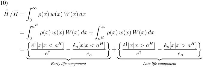
4.3 Decomposition of the relative derivative ofH
The relative derivative ofHdefined in Equation (1) can be decomposed between compo-nents before and after the threshold ageaHas follows:
˙
H /H= Z ∞
0
ρ(x)w(x)W(x)dx
= Z aH
0
ρ(x)w(x)W(x)dx+ Z ∞
aH
ρ(x)w(x)W(x)dx
=
e˙†[x|x < aH] e† −
˙
eo[x|x < aH] eo
| {z }
Early life component
+
e˙†[x|x > aH] e† −
˙
eo[x|x > aH] eo
| {z }
Late life component (10)
5. Conclusion
Several authors have been interested in decomposing changes over time in life expectancy (Arriaga 1984; Vaupel 1986; Pollard 1988; Vaupel and Canudas-Romo 2003; Beltr´an-S´anchez, Preston, and Canudas-Romo 2008; Beltr´an-S´anchez and Soneji 2011). Most recently, scholars have also investigated how life disparity fluctuations over time can be decomposed (Zhang and Vaupel 2009; Wagner 2010; Shkolnikov et al. 2011; Aburto and van Raalte 2018; Aburto and Beltr´an-S´anchez 2019). Here, we bring both perspectives together and shed light on the dynamics behind changes in the lifetable entropy.
Leser (1955) first derived the lifetable entropy as the elasticity of life expectancy. Keyfitz (1977) proposedHas a lifetable function “that measures the change in life ex-pectancy at birth consequent on a proportional change in age-specific rates” (Keyfitz 1977: 413). Since then, several authors have been interested in this measure and its use (Demetrius 1978, 1979; Mitra 1978; Goldman and Lord 1986; Vaupel 1986; Hakkert 1987; Hill 1993; Fern´andez and Beltr´an-S´anchez 2015). Even though the lifetable en-tropy and e† are both measures of lifespan variation, their demographic interpretation
differs. The former is defined as the elasticity of life expectancy due to changes in death rates (Keyfitz 1968) whereas the latter one refers to the average years lost due to death (Vaupel, Zhang, and van Raalte 2011). The life table entropy measures relative variability, whilee†measures absolute lifespan variation. Therefore, the lifetable entropy is appro-priate to compare different shapes of age-at-death distributions across different species and over time (Baudisch 2011; Wrycza, Missov, and Baudisch 2015), whilee† has been used to obtain insights about lifespan variation in different countries and in subpopula-tion groups, for instance by occupasubpopula-tional class or income (van Raalte, Martikainen, and Myrskyl¨a 2014; Brønnum-Hansen 2017). Both measures are meaningful and comple-mentary, but the calculation of their threshold ages should be performed accordingly to correctly interpret changes of age patterns of mortality.
References
Aburto, J.M. and Beltr´an-S´anchez, H. (2019). Upsurge of homicides and its impact on life expectancy and life span inequality in Mexico, 2005–2015. American Journal of Public Health109(3): 483–489.doi:10.2105/AJPH.2018.304878.
Aburto, J.M. and van Raalte, A.A. (2018). Lifespan dispersion in times of life expectancy fluctuation: The case of Central and Eastern Europe. Demography55(6): 2071–2096.
doi:10.1007/s13524-018-0729-9.
Aburto, J.M., Wensink, M., van Raalte, A., and Lindahl-Jacobsen, R. (2018). Potential gains in life expectancy by reducing inequality of lifespans in Denmark: An inter-national comparison and cause-of-death analysis. BMC Public Health18(1): 831.
doi:10.1186/s12889-018-5730-0.
Alvarez, J., Aburto, J., and Canudas-Romo, V. (2019). Latin american convergence and divergence towards the mortality profiles of developed countries. Population Studies
1–18.doi:10.1080/00324728.2019.1614651.
Archer, C.R., Basellini, U., Hunt, J., Simpson, S.J., Lee, K.P., and Baudisch, A. (2018). Diet has independent effects on the pace and shape of aging in Drosophila melanogaster.Biogerontology19(1): 1–12. doi:10.1007/s10522-017-9729-1.
Arriaga, E.E. (1984). Measuring and explaining the change in life expectancies. Demog-raphy21(1): 83–96. doi:10.2307/2061029.
Baudisch, A. (2011). The pace and shape of ageing. Methods in Ecology and Evolution
2(4): 375–382.doi:10.1111/j.2041-210X.2010.00087.x.
Baudisch, A., Salguero-G´omez, R., Jones, O.R., Wrycza, T., Mbeau-Ache, C., Franco, M., and Colchero, F. (2013). The pace and shape of senescence in angiosperms. Jour-nal of Ecology101(3): 596–606.doi:10.1111/1365-2745.12084.
Beltr´an-S´anchez, H., Preston, S.H., and Canudas-Romo, V. (2008). An integrated ap-proach to cause-of-death analysis: Cause-deleted life tables and decompositions of life expectancy. Demographic Research19(35): 1323–1350. doi:10.4054/DemRes.2008.
19.35.
Beltr´an-S´anchez, H. and Soneji, S. (2011). A unifying framework for assessing changes in life expectancy associated with changes in mortality: The case of violent deaths.
Theoretical Population Biology80(1): 38–48. doi:10.1016/j.tpb.2011.05.002.
Brønnum-Hansen, H. (2017). Socially disparate trends in lifespan variation: A trend study on income and mortality based on nationwide danish register data. BMJ Open
Burger, O., Baudisch, A., and Vaupel, J.W. (2012). Human mortality improvement in evo-lutionary context. Proceedings of the National Academy of Sciences109(44): 18210– 18214.doi:10.1073/pnas.1215627109.
Colchero, F., Rau, R., Jones, O.R., Barthold, J.A., Conde, D.A., Lenart, A., N´emeth, L., Scheuerlein, A., Schoeley, J., Torres, C., Zarulli, V., Altmann, J., Brockman, D.K., Bronikowski, A.M., Fedigan, L.M., Pusey, A.E., Strier, K.B., Baudisch, A., Alberts, S.C., and Vaupel, J.W. (2016). The emergence of longevous popula-tions. Proceedings of the National Academy of Sciences 113(48): e7681–e7690.
doi:10.1073/pnas.1612191113.
Demetrius, L. (1974). Demographic parameters and natural selection.Proceedings of the National Academy of Sciences71(12): 4645–4647.doi:10.1073/pnas.71.12.4645.
Demetrius, L. (1978). Adaptive value, entropy and survivorship curves. Nature275: 213–214.doi:10.1038/275213a0.
Demetrius, L. (1979). Relations between demographic parameters. Demography16(2): 329–338.doi:10.2307/2061146.
Edwards, R.D. and Tuljapurkar, S. (2005). Inequality in life spans and a new perspective on mortality convergence across industrialized countries.Population and Development Review31(4): 645–674. doi:10.1111/j.1728-4457.2005.00092.x.
Fern´andez, O.E. and Beltr´an-S´anchez, H. (2015). The entropy of the life table: A reap-praisal.Theoretical Population Biology104: 26–45. doi:10.1016/j.tpb.2015.07.001.
Gigliarano, C., Basellini, U., and Bonetti, M. (2017). Longevity and concentration in survival times: The log-scale-location family of failure time models. Lifetime Data Analysis23(2): 254–274. doi:10.1007/s10985-016-9356-1.
Gillespie, D.O., Trotter, M.V., and Tuljapurkar, S.D. (2014). Divergence in age patterns of mortality change drives international divergence in lifespan inequality.Demography
51(3): 1003–1017. doi:10.1007/s13524-014-0287-8.
Goldman, N. and Lord, G. (1986). A new look at entropy and the life table.Demography
23(2): 275–282. doi:10.2307/2061621.
Hakkert, R. (1987). Life table transformations and inequality measures: Some notewor-thy formal relationships. Demography24(4): 615–622. doi:10.2307/2061396.
Hill, G. (1993). The entropy of the survival curve: An alternative measure. Canadian Studies in Population20(1): 43–57. doi:10.25336/P6830H.
Keyfitz, N. (1968). Introduction to the mathematics of populations. Reading: Addison– Wesley.
Keyfitz, N. (1977). What difference would it make if cancer were eradicated? An exami-nation of the Taeuber paradox.Demography14(4): 411–418. doi:10.2307/2060587.
Leser, C. (1955). Variations in mortality and life expectation. Population Studies9(1): 67–71.doi:10.1080/00324728.1955.10405052.
Missov, T.I. and Lenart, A. (2013). Gompertz–Makeham life expectancies: Expressions and applications. Theoretical Population Biology90: 29–35. doi:10.1016/j.tpb.2013.
09.013.
Mitra, S. (1978). A short note on the Taeuber paradox. Demography15(4): 621–623.
doi:10.2307/2061211.
Pollard, J.H. (1988). On the decomposition of changes in expectation of life and differ-entials in life expectancy. Demography25(2): 265–276. doi:10.2307/2061293.
Shkolnikov, V.M., Andreev, E.M., and Begun, A.Z. (2003). Gini coefficient as a life table function: Computation from discrete data, decomposition of differences and empirical examples.Demographic Research8(11): 305–358. doi:10.4054/DemRes.2003.8.11.
Shkolnikov, V.M., Andreev, E.M., Zhang, Z., Oeppen, J., and Vaupel, J.W. (2011). Losses of expected lifetime in the United States and other developed countries: Methods and empirical analyses.Demography48(1): 211–239. doi:10.1007/s13524-011-0015-6.
Smits, J. and Monden, C. (2009). Length of life inequality around the globe. Social Science and Medicine68(6): 1114–1123.doi:10.1016/j.socscimed.2008.12.034.
Tuljapurkar, S. and Edwards, R.D. (2011). Variance in death and its implications for modeling and forecasting mortality. Demographic Research24(21): 497–526.
doi:10.4054/DemRes.2011.24.21.
van Raalte, A.A. and Caswell, H. (2013). Perturbation analysis of indices of lifespan variability.Demography50(5): 1615–1640.doi:10.1007/s13524-013-0223-3.
van Raalte, A.A., Martikainen, P., and Myrskyl¨a, M. (2014). Lifespan variation by oc-cupational class: compression or stagnation over time? Demography51(1): 73–95.
doi:10.1007/s13524-013-0253-x.
van Raalte, A.A., Sasson, I., and Martikainen, P. (2018). The case for monitoring life-span inequality.Science362(6418): 1002–1004. doi:10.1126/science.aau5811.
Vaupel, J.W. (1986). How change in age-specific mortality affects life expectancy. Pop-ulation Studies40(1): 147–157. doi:10.1080/0032472031000141896.
bouquet of formulas in honor of Nathan Keyfitz’s 90thbirthday. Demography40(2): 201–216.doi:10.1353/dem.2003.0018.
Vaupel, J.W., Zhang, Z., and van Raalte, A.A. (2011). Life expectancy and dispar-ity: An international comparison of life table data. BMJ Open e000128: 1–6.
doi:10.1136/bmjopen-2011-000128.
Wagner, P. (2010). Sensitivity of life disparity with respect to changes in mortality rates.
Demographic Research23(3): 63–72. doi:10.4054/DemRes.2010.23.3.
Wrycza, T. (2014). Entropy of the Gompertz–Makeham mortality model. Demographic Research30(49): 1397–1404.doi:10.4054/DemRes.2014.30.49.
Wrycza, T.F., Missov, T.I., and Baudisch, A. (2015). Quantifying the shape of aging.
PLoS ONE10(3): e0119163.doi:10.1371/journal.pone.0119163.
Zhang, Z. and Vaupel, J.W. (2009). The age separating early deaths from late deaths.
Appendix
Proposition 1
Let e†(x) = R∞
x d(a)e(a)da / `(x) be a measure of lifespan disparity above age x, whered(a)accounts for the distribution of deaths,e(a)the remaining life expectancy at agea, and`(x)is the probability of surviving from birth to agex. Then,
(A1) e†(x) = 1
`(x) Z ∞
x
`(a) H(a)−H(x)da,
whereH(x)is the cumulative hazard to agex.
Proof. Note that
1
`(x) Z ∞
x
`(a) H(a)−H(x)da= 1
`(x) Z ∞
x `(a)
Z a
x
µ(y)dy da,
where functionµ(y)is the force of mortality or hazard rate. By reversing the order of integration, and using thate(y) =Ry∞`(a)da / `(y)andd(y) =µ(y)`(y), we get
1
`(x) Z ∞
x `(a)
Z a
x
µ(y)dy da= 1
`(x) Z ∞
x µ(y)
Z ∞
y
`(a)da dy
= 1
`(x) Z ∞
x
µ(y)`(y)e(y)dy
= 1
`(x) Z ∞
x
d(y)e(y)dy
=e†(x),
which proves (A1).
Proposition 2
Let`(x)be the probability of surviving from birth to agex. LetHbe the lifetable entropy andH(x) =e†(x)/ e(x)the lifetable entropy conditioned on reaching agex. LetH(x)
be the cumulative hazard to agex. Then,g(x) := H(x) +H(x)−1−H is a strictly increasing function.
Proof. In order to demonstrate thatg(x)is a strictly increasing function it is sufficient to show that its first derivative is always positive. We must prove that
(A2) ∂
∂xg(x) = ∂
∂x H(x) +H(x)−1−H
= ∂
∂xH(x) + ∂
for all agesx.
By the fundamental theorem of calculus,
(A3) ∂
∂xH(x) = ∂ ∂x
Z x
0
µ(a)da=µ(x),
whereas
∂
∂xH(x) = ∂ ∂x
e†(x)
e(x)
= 1
e(x)2
e(x) ∂
∂xe
†(x)−e†(x) ∂
∂xe(x)
.
First, note that
∂ ∂xe
†(x) = ∂
∂x
1
`(x) Z ∞
x
d(a)e(a)da
= 1
`(x)2
`(x) ∂
∂x
Z ∞
x
d(a)e(a)da
−
Z ∞
x
d(a)e(a)da ∂ ∂x`(x)
= 1
`(x)2
`(x) −d(x)e(x)−
Z ∞
x
d(a)e(a)da −µ(x)`(x)
=−µ(x)`(x)e(x) `(x) +µ(x)
R∞
x d(a)e(a)da `(x) =µ(x) e†(x)−e(x)
.
(A4)
On the other hand,
∂
∂xe(x) = ∂ ∂x
1
`(x) Z ∞
x
`(a)da
= 1
`(x)2
`(x) ∂
∂x
Z ∞
x
`(a)da
−
Z ∞
x
`(a)da ∂ ∂x`(x)
= 1
`(x)2
`(x) −`(x)
−
Z ∞
x
`(a)da −µ(x)`(x)
=e(x)µ(x)−1.
(A5)
Therefore, using (A4) and (A5), we get
∂
∂xH(x) =
1
e(x)2
e(x)µ(x) e†(x)−e(x)
−e†(x) e(x)µ(x)−1
= 1
e(x)2 e
†(x)e(x)µ(x)−e(x)2µ(x)−e†(x)e(x)µ(x) +e†(x)
= e
†(x)
e(x)2 −µ(x).
Finally, replacing (A3) and (A6) in (A2) yields
∂
∂xg(x) =µ(x) + e†(x)
e(x)2 −µ(x) =
e†(x)
e(x)2 >0,
which holds true for all ages since by definitione†(x)>0for allx≥0. Hence,g(x)is
a strictly increasing function.
Proposition 3
Assume the force of mortality follows a Gompertz distribution with hazardµ(x) =αeβx, wherex ≥ 0 denotes the age andα,β > 0 are parameters. Suppose mortality im-provements over time occur at all ages, therefore there is a unique threshold ageaHthat separates positive from negative contributions to the lifetable entropyH. Then,aH is approximately proportional to the life expectancy at birtheo.
Proof. The cumulative hazard of the Gompertz model is given by
H(x) = α
β e βx
−1 ,
wherex≥ 0denotes the age andα,β >0are parameters. Following Wrycza (2014), the lifetable entropy can be expressed in terms of the Gompertz parameters as
H= 1
β 1 eo −α ,
whereeo is the life expectancy at birth. Plugging these two expressions into function g(x)from Equation (9) yields
(A7) g(x) = 1
β
αeβx− 1 eo
+H(x)−1.
From Equation (A1) in Proposition 1, the lifetable entropy conditioned on surviving to agexcan be expressed as
H(x) =e †(x)
e(x) = R∞
x `(a) H(a)−H(x)
da
R∞
x `(a)da
.
Using the above expressions in terms of the Gompertz parameters, it holds that the lifetable entropy conditioned on surviving to agexis
H(x) = R∞
x `(a) α β e
βa−eβx
da
R∞
x `(a)da
= R∞
x `(a)αe βada βR∞
x `(a)da −α
βe βx
= R∞
x `(a)µ(a)da β e(x)`(x) −
α βe
βx= 1 β
1
e(x)−αe
βx
.
The last step in (A8) uses the product`(a)µ(a)as the age-at-death distribution, which then implies thatRx∞`(a)µ(a)da=`(x). Thus,g(x)in (A7) reduces to
(A9) g(x) = 1
β
1
e(x)− 1
eo
−1,
wheree(x)is the remaining life expectancy at agex. Equation (A9) implies that the threshold ageaHof the lifetable entropyHunder the Gompertz model occurs whenever
e(x) = eo
β eo+ 1
.
Following Missov and Lenart (2013), the remaining life expectancy at agexin the Gompertz case can be approximated by
(A10) e(x)≈ 1
β e
α/β −γ−ln(α/β)−β x ,
whereγ ≈0.57722is the Euler–Mascheroni constant. Hence, the threshold age occurs whenever
e(x)≈ 1 βe
α/β −γ−ln(α/β)−β x
= eo
β eo+ 1 ⇐⇒x=−e
−α/βe
o β eo+ 1
− 1
β γ+ ln(α/β)
.
Note that (A10) implies thateo≈eα/β −γ−ln(α/β)
/ β. Using this approxi-mation,
aH ≈ − e
−α/βe
o
eα/β (−γ−ln (α / β)) + 1+ eo
eα/β
= eo
eα/β
1
eα/β(γ+ ln (α / β))−1 + 1
=eo
γ+ ln(α/β)
eα/β(γ+ ln (α / β))−1
=eo·δ, (A11)
which proves that the threshold ageaHof the lifetable entropyHfor the Gompertz model is (approximately) proportional toeoby a factorδthat only depends on parametersα,β,