On the terms of geomagnetic daily variation in Antarctica

www.ann-geophys.net/27/2483/2009/

© Author(s) 2009. This work is distributed under the Creative Commons Attribution 3.0 License.

Annales

Geophysicae

On the terms of geomagnetic daily variation in Antarctica

P. De Michelis, R. Tozzi, and A. Meloni

Istituto Nazionale di Geofisica e Vulcanologia, Roma, Italy

Received: 5 November 2008 – Revised: 14 May 2009 – Accepted: 1 June 2009 – Published: 22 June 2009

Abstract. The target of this work is to investigate the nature of magnetic perturbations produced by ionospheric and mag-netospheric currents as recorded at high-latitude geomag-netic stations. In particular, we investigate the effects of these currents on geomagnetic data recorded in Antarctica. To this purpose we apply a mathematical method, known as Natu-ral Orthogonal Composition, to analyze the magnetic field disturbances along the three geomagnetic field components (X, Y andZ) recorded at Mario Zucchelli Station (IAGA code TNB; geographic coordinates: 74.7◦S, 164.1◦E) from 1995 to 1998. Using this type of analysis, we characterize the dominant modes of the geomagnetic field daily variabil-ity through a set of empirical orthogonal functions (EOFs). While such mathematically independent EOFs do not neces-sarily represent physically independent modes of variability, we find that some of them are actually related to well known current patterns located at high latitudes.

Keywords. Geomagnetism and paleomagnetism (Time vari-ations, diurnal to secular) – Magnetospheric physics (Polar cap phenomena; Solar wind-magnetosphere interactions)

1 Introduction

Continuous recordings of the elements of the Earth’s mag-netic field at ground-based observatories show that these el-ements rarely remain constant for more than an hour or two and if it happens it is generally during the night. In fact, mag-netograms are usually characterized by random fluctuations superimposed on a regular trend that is a function of local time, i.e. the solar quiet daily variationSq.

Unfortunately, since the daily record of geomagnetic vari-ations results from the overlapping of magnetic fields

pro-Correspondence to: P. De Michelis ([email protected])

duced by different sources, external as well as internal to the Earth, it is extremely difficult to sort out the single contribu-tions. Here, we are interested mainly in those electric current systems, existing in the polar regions, that generate the daily variation.

Indeed, the study of the daily variation above 60◦_magnetic

latitude is of great importance in understanding the polar cap current systems and the role that these current systems play in the magnetosphere-ionosphere electrodynamic coupling at high latitudes being these current systems mainly driven by particle precipitation and field-aligned currents and depend-ing their configuration on solar wind parameters, magnetic activity and ionospheric electrical conductivity.

In the past, Hasegawa (1939) was the first to find a signifi-cant difference between theSqvariations in the polar region

and those which were expected to arise from the upper atmo-sphere dynamo process. Later, analyzing geomagnetic data in both Arctic and Antarctic regions, Nagata and Kokubun (1962) found that the geomagnetic daily variation field in the polar cap on geomagnetically quiet days consisted not only of the well establishedS_q0field, which is a smooth ex-trapolation to the polar region ofSq defined at mid and low

latitudes, but also of an additional field, theSqp field. In

de-tail, they showed that the associatedSqp equivalent current

consisted of two parts. One was the dynamo induced cur-rent across the pole, approximately from dawn to dusk. The other consisted of two current cells, a counterclockwise cell in the afternoon-evening sector and a clockwise cell in the forenoon-morning sector. Since then the Sqp variation has

been studied extensively by a number of scientists who at-tempted to find a three-dimensional current system for the Sqpvariation.

At present, it is known that theSpqfield is mainly generated

depend on the season. Indeed, in summer the evening cell is much wider and stronger (up to three times) than the morning one, while in winter the two cells are more similar. It is be-lieved that theSqpcurrent system, contrary to theS0qsystem,

is not driven by a ionospheric dynamo due to solar photoion-ization and tides but rather by external sources (essentially located in the magnetosphere). The pattern of this current system is partially modified by the processes that happen in the magnetosphere and by its interaction with the interplan-etary magnetic field (IMF). Indeed, the currents flowing in and near the polar cusp and in the dayside polar cap are cou-pled, through the field-aligned currents, with the magneto-spheric currents. It is for this reason that theSqpcurrent

sys-tem is strongly enhanced and modified during geomagnetic disturbances and auroral substorms when the effects of non-vanishing transverse IMF components are superimposed to the quiet time configuration of the current system. However, the fact that a twin vortex system appears to be present above 70◦of latitude for all orientations of the IMF, indicates that some elements of the current pattern may be independent of the IMF (Friis-Christensen et al., 1985) and it is this portion of the current system that is the real quiet part of the polar equivalent current system. In the polar regions, however, the quiet-time magnetosphere-ionosphere condition occurs only when the energy transfer from the solar wind to the magne-tosphere is at a minimum and even during such quiet condi-tions, the geomagnetic field at high latitudes is continuously disturbed. Consequently, in these regions quiet days are quite rare events.

Recently, Xu and Kamide (2004) and Chen et al. (2007) have applied a technique, the Natural Orthogonal Compo-nent (NOC) analysis, to separate and recognize the differ-ent contributions of the ionospheric-magnetospheric currdiffer-ent systems to the daily changes of the geomagnetic field as recorded at mid-latitude ground-based geomagnetic observa-tories. Using this method of analysis, the authors have been able to separate the solar quiet daily variation along theH component from other complicated disturbances. We have extended these works at high latitudes analyzing the hourly values of the three magnetic field components (X,Y andZ) recorded at the Italian geomagnetic observatory TNB located in Antarctica during a period of 4 years (1995–1998). In-deed, the diurnal variation of the geomagnetic field elements is still not completely understood at high latitudes where the configuration of the electric current systems responsible of the daily geomagnetic field variation is complex. Using the NOC analysis, the time evolution of the geomagnetic field has been studied and it has been found that the first and sec-ond order natural components dominate over higher order components also exhibiting features quite similar to those of Sqpcurrent systems. However, the aim of our study has been

not only to identify the different current systems that con-tribute to the daily variation of the Earth’s magnetic field but also to study their temporal evolution and find possible corre-lations with appropriate parameters related to these currents.

2 Data set and method of analysis

To study the geomagnetic field daily variation in the Antarc-tic region we used the hourly mean values of the three mag-netic field elements which completely describe the magmag-netic field vector recorded at Terra Nova Bay in Antarctica from 1995 to 1998 (Villante et al., 1997). The geographic and cor-rected geomagnetic coordinates of Mario Zucchelli geomag-netic observatory at Terra Nova Bay (IAGA code TNB) are 74.7◦S, 164.1◦E and 77.27◦S, 278.6◦E (IGRF95), respec-tively, while the geographic local time (LT) and corrected magnetic local time (MLT) respect to universal time (UT) are LT=UT+11 and MLT=UT-8 according to NASA service http://omniweb.gsfc.nasa.gov/vitmo/cgm vitmo.html.

At this geomagnetic observatory, three-axis flux gate mag-netometers oriented in the reference system H DZ are in-stalled. Consequently at TNB observatory, the magnetic field is measured in a coordinate system where theH component point towards magnetic north, theDcomponent to magnetic east, and the Z component is orthogonal to both of them, pointing downward. The orientation of this kind of coordi-nate system therefore depends on the location the magnetic field is being measured at.

In this study we have transformed the geomagnetic field horizontal components (H and D) into X and Y compo-nents, which are directed along the geographic meridian and parallel, respectively. As angular rotation between the geo-graphic and magnetic meridian, we have considered the av-erage value of the declination angleD at TNB observatory, which is equal to 136◦. This transformation is necessary be-ing the reconstruction of the equivalent current systems in the polar region generally obtained from theX,Y andZ mag-netic field values. Indeed, it is known that there is a consid-erable deviation between the direction of theH component (magnetic north) and theX component (geographic north) especially in the higher-latitudes observatories. At high lati-tudes the magnetic perturbation in the geographic northward component depends almost equally on the magnetic pertur-bation alongH andD and even the sign of the magnetic perturbation alongXcan be opposite to the sign of the per-turbation alongH. For this reason, to compare our results with those obtained using different methods of analysis, it is important to use the same reference system.

1992; Xu and Kamide, 2004) can be a tool extremely useful to reveal simple patterns within it.

The Natural Orthogonal Component (NOC) analysis is, in-deed, a powerful and elegant method of data analysis aimed at obtaining low-dimensional approximate descriptions of high-dimensional processes. In particular, this method of analysis offers a way to extract those structures that remain coherent throughout a time series. In practice, given a set of observations it is possible to estimate a set of indepen-dent eigenvectors and eigenvalues whose combination allows writing the observed variables in terms of a new basis that is just a rotated version of the original observations. This type of analysis has been developed by several authors and widely used in literature, for instance for the study of daily magnetic variation (Golovkov et al., 1978; Xu and Kamide, 2004; Chen et al. 2007), for the study of global models of the geomagnetic field (Xu, 2002, 2003), for the automatic com-putation ofKindices (Golovkov et al., 1989; Papitashvili et al., 1992), and even for the separation of the substorm cur-rent system into directly driven and loading-unloading com-ponents (Sun et al., 1998, 2000).

Before describing the application of the NOC method to our data set, a brief introduction follows. Let us suppose to have a variablex(di,tj)representing the value of a magnetic

field element (X, Y, Z) for a certain daydi, and time tj.

Given a number of samples ofx(di,tj)at different days and

times, the application of the NOC method allows extracting a smaller set of variables, let’s say of Empirical Orthogonal Functions (EOFs) and Principal Components (PCs), able to describe the whole set of observations. Among the differ-ent techniques used for data represdiffer-entation the NOC method has the peculiarity that the set of functions used for the ex-pansion of the time series is estimated using only the ob-served dataset. This is the main difference with other meth-ods, as for instance the spherical harmonic and Fourier analy-ses, where the fundamental orthogonal basis set is artificially chosen a priori.

Therefore, we can decompose the daily variation of any geomagnetic component in terms of a basis of Empirical Or-thogonal Functions (EOFs)φk(tj):

x(di,tj)= K X

k=1

wkAk(di)φk(tj) (1)

where the collection of valuesx(di,tj)are the elementsxij

of the matrix X (m×n)whose rows correspond to the days (i=1, 2, . . . .,m)and columns correspond to the time (j=1, 2, . . . ., n), K is the number of components chosen for the decomposition (i.e. the truncation level),φk(tj)is the mode

(EOF) of thek-th component describing the daily variation (i.e. is the basis used for the expansion),Ak(di)is the

Prin-cipal Component (PC) and represents the amplitude ofk-th mode, andwkis the associated weigh.

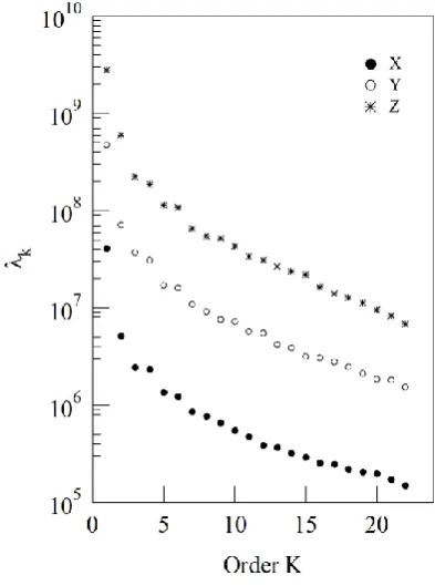
To evaluate the EOFs and the associated PCs from a dataset the error made in the representation of the observed

Fig. 1. The NOC eigenvalue spectraλk ofX,Y andZmagnetic

field components recorded at Mario Zucchelli Station (TNB) in Antarctica. Theλkspectra ofYandZcomponents have been scaled

by a factor of 10 and 102, respectively, for convenience.

data by means of the expansion (1) is to be minimized. This error depends on the truncation levelK: the higher the trun-cation level, the lower the error.

Since we are looking for a number of components able to describe completely the observed variable, one additional as-sumption is that the EOFs (φk)are orthogonal and the PCs (Ak)vary independently. This leads to solve the well-known eigenvalue-eigenvector problem that permits an estimation of the eigenvaluesλk (λk=1/wk ) together with the

corre-sponding eigenvectorsφkand amplitudesAkfork=1, . . . ,K (see for more details Xu and Kamide, 2004).

In what follows we try to find a correspondence between the main EOFs and the real current patterns flowing in the ionosphere and magnetosphere in the polar region. However, it is important to underline that the EOFs and PCs found in this way do not necessarily correspond to real current sys-tems. In fact, while the EOFs are orthogonal by definition, the currents are generally not.

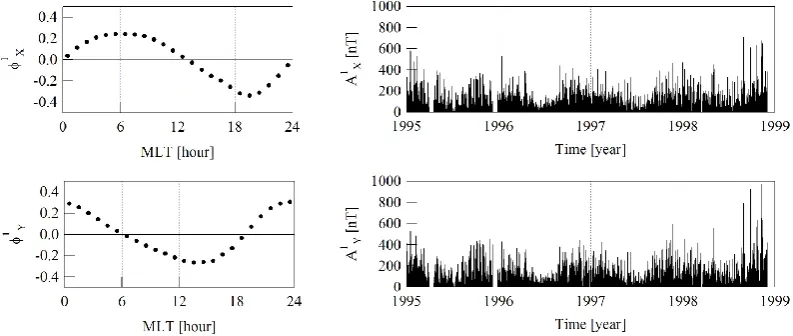
Fig. 2. On the left, the first EOF associated to theX(top) andY (bottom) components, respectively; on the right, their associated PCs.

3 Results and discussion

As already mentioned in the previous section, we used the hourly average values of the variations of theX,Y andZ magnetic field components recorded at TNB geomagnetic observatory from 1 January 1995 to 30 November 1998. On the long term side these data are characterized by annual as well as secular changes. For this reason, before applying the NOC analysis, we have removed the daily mean from each day eliminating, in this way, the trend caused by the secular changes and other possible long term drift.

Figure 1 shows the spectra of the eigenvaluesλk obtained

applying the NOC analysis to the three magnetic field ele-ments. A rapid drop characterizes all spectra, and the energy is mainly concentrated in the lowest orders. As a matter of fact, the first two eigenvalues (and consequently the two as-sociated PCs) explain up to 77%, 76% and 75% of the total variance ofX,Y andZmagnetic field elements, respectively. This implies that the first few EOFs play a role much more relevant than the others and, consequently, the daily variation of the geomagnetic field at high latitudes can be well recon-structed by considering only these few NOC terms.

In Figs. 2, 3 and 4, we have grouped the EOFs and PCs according to the different current systems we think they may represent. Since we believe that the first (k=1) EOF as-sociated toX andY elements (φ_X1 andφ_Y1)may represent the Sqpcurrent system, we have grouped them and the

cor-responding PC (φ_X1 andφ_Y1)in Fig. 2. Indeed, if we take into account the different directions assumed by the two EOFs simultaneously in the different magnetic local time sectors (00:00–06:00; 06:00–12:00; 12:00–18:00 and 18:00– 24:00) we can easily reconstruct the pattern of the current system underneath which TNB geomagnetic observatory ro-tates. The pattern so inferred consists of two currents flowing in opposite directions from 24:00 to 12:00 MLT, one crossing 18:00 MLT and the other 06:00 MLT. This result is well in

agreement with the structure of theSqpcurrent system, which

is formed by two vortices where the currents flow in opposite directions. Indeed, what we are able to reconstruct from our dataset is only the outer portion of this current system. The PCs (A1_XandA1_Y)associated to these EOFs are plotted in the right panels of the same figure. These components display a seasonal trend characterized by a maximum in the austral summer and a minimum in the austral winter. This seasonal trend is in agreement with the characteristic of theSqp field

intensity to show a strong seasonal variation. Indeed, while the total current associated to theSqpsystem amounts to about

15×104A in the sunlit polar cap (summer), it is reduced to less than one third of its value when the polar cap becomes dark (winter) (Xu, 1989).

It should be pointed out that, in addition to its seasonal variation, Sqp depends on magnetic activity and IMF sector

polarity. Indeed, it has been shown that when magnetic activ-ity increases, theSqpcurrent pattern is distorted while the

po-sition of the vortices is shifted toward either the morning side or evening side according to sector polarities of IMF (Friis-Christensen, 1984). We have analysed the existence of this possible relationship studying the correlation between the PCs (A1_XandA1_Y)and some significant parameters: the solar wind dynamic pressurePdyn(Pdyn=ρv2, whereρis the

so-lar wind mass density andvis its flow speed), the north-south component (Bz), the southward (BS)and the eastward (By)

components of the interplanetary magnetic field (IMF) in the GSM system, the so-called energy coupling functionε (Aka-sofu, 1978), which is a measure of the energy flux that flows into the magnetosphere, and theKp index, which is an

indi-cation of the level of geomagnetic perturbation on planetary scale (data come from OMNI2 database).

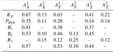
Fig. 3. On the left, the second EOF associated to theX(top) andY (bottom) components, respectively. On the right, the PCs associated to each EOF.

linear relationship between the analyzed variables, while a value of 0 is the result of no linear relationship. In prac-tice, the value of this parameter is some intermediate number whose significance depends on the number of samples.

In order to establish a significance level for the correla-tion found, we have fixed a threshold|rs|for the Pearson’s

coefficient. This threshold has been evaluated according to the significance level of 1% for samples characterized by a degree of freedom equal to 1000. The chosen threshold is |rs|=0.081 (Fisher, 1972). It means that in our case values

smaller than 0.081 can be read as absence of correlation. In Table 1 we have reported the correlation coefficients between the PCs and the selected parameters. It is necessary to notice that the correlation between a PC and one param-eter will be found only if this paramparam-eter produces a change in the intensity of the current system described by the EOF associated to the PC. Indeed, the PC describes the temporal evolution of a specific spatial mode, i.e. EOF, and it cannot consequently describe any distortion of the current system due to different magnetospheric configuration.

According to the results reported in Table 1, the first PC associated to theXcomponent (A1_X)is very well correlated withKp,Bz,Bs,ε, andPdyn. The same results have been

obtained correlating the PC associated to theY component (A1_Y)with the same parameters (data reported in Table 1). These results support the hypothesis that the first (k=1) EOFs associated toX andY components (φ_X1 andφ_Y1)may repre-sent theSqpcurrent system. Indeed, the selected parameters,

well characterizing the impact of the solar wind on the mag-netosphere, can affect theSqpcurrent pattern.

It is worth noticing that this result is in agreement with the reconstruction of equivalent ionospheric currents above Antarctica proposed by Papitashvili et al. (1990). Using hourly mean values of geomagnetic field horizontal compo-nentsX and Y from 20 Antarctic observatories and

auto-Table 1. The Pearson’s|r|linear coefficient. The “–“ refers to values less than the fixed threshold value|rs|=0.081.

A1_X A2_X A1_Y A2_Y A1_Z A2_Z Kp 0.67 0.13 0.63 – 0.41 0.22

Pdyn 0.35 0.11 0.28 – 0.14 0.14

Bz 0.41 – 0.38 – 0.37 –

Bs 0.53 0.10 0.46 0.13 0.45 –

By – 0.15 0.12 0.25 – 0.12

ε 0.57 – 0.53 0.10 0.44 –

matic stations, Papitashvili et al. (1990) have recognized the existence of three different types of ionospheric convection patterns: a) a two-vortex system controlled by the “quasi-viscous” interaction and southward IMF; b) a zonal current system, controlled by azimuthal IMF; and c) a two-vortex system controlled by the northward IMF.

According to this analysis our first mode, associated to the XandY components (φ_X1 andφ_Y1), seems to identify the first type of the equivalent current system found by Papitashvili et al. (1990).

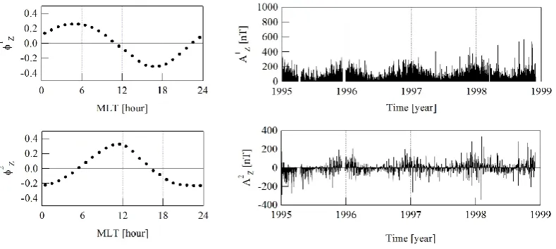
Fig. 4. On the left, the first (top) and the second (bottom) EOF associated to theZcomponent. On the right, the PCs associated to each EOF.

What is interesting to notice is that the PCsA2_XandA2_Y, associated to the EOFs φ_X2 and φ_Y2, are weakly correlated with some interplanetary quantities (see Table 1) and in par-ticular these PCs are correlated to the daily average direc-tion of theBy component of the IMF. The current system,

which is described by the second EOFs associated to the X and Y components of the geomagnetic field, seems to be consequently influenced by the Svalgaard-Mansurov ef-fect (Svalgaard, 1968; Mansurov, 1969). According to this effect, indeed, the ground-based geomagnetic observations and in particular the daily variation of the geomagnetic field at high (cusp and polar cap) latitudes are influenced by the heliospheric magnetic field sector polarity being the sign of theBy responsible for the direction of the east-west flowing

ionospheric current. This correlation is not so obvious for a current system that should represent the Pedersen currents. It is known indeed that the pattern of the Pedersen currents does not change its direction and it cannot be consequently influenced by theBy component of the IMF. However, we

know that in the polar cap exists a zonal current around the geomagnetic pole (see for example Papitashvili et al., 1990), which flows anticlockwise forBy>0 and in the opposite

di-rection forBy<0. We can suppose that the EOFsφX2 and φ_Y2, in addition to the Pedersen currents, contain this zonal current system, which the NOC analysis is not able to recog-nize and separate.

Figure 4 shows the trends of the first (φ_Z1) and second (φ_Z2)EOFs associated to theZcomponent in magnetic local time (MLT). The daily trend of theφ1_Zis characterized by a maximum in the morning sector and a minimum in the after-noon one while theφ2_Zfunction displays a single maximum at around noon.

The recognition of the current systems associated to these EOFs is not simple. From a theoretical point of view, if we divide the current systems responsible of the geomagnetic variations into toroidal and poloidal systems, we have that

the toroidal current flowing in the ionosphere sheet layer will produce poloidal magnetic perturbations while the poloidal one, consisting of field-aligned currents and their closing ir-rotational currents in the ionospheric current sheet, will pro-duce toroidal magnetic perturbations above the ionosphere and no perturbations below (Richmond, 2002). This means that the ground-based magnetometers should respond almost exclusively to poloidal magnetic fields due to the solenoidal current circuit while they shouldn’t measure those toroidal fields due to the poloidal current circuit.

At high latitudes as poloidal current circuits we have mainly the Hall and Pedersen currents. The Pedersen cur-rent is perpendicular to theZaxis and parallel to the electric field created by the field-aligned currents, while the Hall cur-rent is perpendicular to both theZaxis and the electric field (Tascione, 1988).

However, analysing the effect of these current systems on theZcomponent of the geomagnetic field it is important to say that according to the Fukushima theorem (Fukushima, 1976), under the assumption of field-aligned currents (FAC) parallel to theZaxis and a ionosphere with uniform conduc-tivity parallel to the ground, the field-aligned and Pedersen currents combined will produce no ground magnetic signa-ture. However, if the inclination of the ambient field deviates slightly from vertical (e.g. inclination≈80◦ at auroral lati-tudes) some magnetic effects from the FAC-Pedersen current circuit will leak to the ground and we will find a small field-aligned contribution from this circuit.

described by the temporal trend of the PC (A1_Z)associated to this EOF (φ1_Z), and it is correlated to theεcoupling func-tion, the southward (Bs), the north-south (Bz) component of

the interplanetary magnetic field, the dynamic pressurePdyn

and theKpindex (see Table 1).

The second natural componentφ_Z2, which is characterized by positive values in the time interval 06:00<MLT<16:00, could be the effect on the ground of the Pedersen currents. Indeed, what is important to notice is that the eigenvalue as-sociated to the second natural component is, in first approxi-mation, one order less than that associated to the first natural component. So, as expected, the perturbation on the ground produced by the Pedersen currents along theZmagnetic field component is small.

4 Summary and conclusions

Ground magnetic perturbations have been widely used to study magnetospheric and ionospheric dynamics, since the magnetic data obtained at the Earth’s surface include valu-able information about a variety of current sources flowing in the ionosphere, magnetosphere, at the magnetopause, and within the Earth’s interior. However, one of the major prob-lems it has always been to evaluate the relative importance of these currents in generating particular patterns or modes of global or local magnetic perturbations under study. We have tried to overcome this problem using the NOC analy-sis. Investigating the nature of the daily magnetic variations recorded at an Antarctic ground observatory, we have found that forX,YandZmagnetic field components the main con-tribution to the polar daily variation comes from the Hall cur-rents. This current system, which is a permanent feature of the polar region, largely depends upon solar wind parameters and magnetospheric conditions. Indeed, we have found that the PCs (A1_X,A1_Y andA1_z), associated to those EOFs (φ_X1,φ_Y1 andφ_Z1)describing the Hall current system, exhibit, as ex-pected, a correlation with the solar wind dynamic pressure (Pdyn), theBz andBs interplanetary magnetic field

compo-nents, the energy coupling functionεand theKpindex. The

second important contribution to the polar daily variation of the geomagnetic field mainly comes from Pedersen currents. However we think that this second mode, obtained from the NOC analysis, may contain also a contribution coming from a zonal current system present at high latitude and controlled by the azimuthal IMF (Papitashvili et al., 1990).

These results, which are well in agreement with the cur-rent systems present at high latitude, show some differences with respect to the results recently presented by Pietrolungo et al. (2008). Indeed, the authors, using data coming from three different geomagnetic observatories all located within the Antarctic polar cap, have suggested that the contribution of theSqppolar electric current systems to the diurnal

varia-tion is not relevant and that the mid latitude ionospheric

cur-rents are the main source of the daily variation also at high latitudes, at least during a period of solar minimum.

On the contrary, according to our analysis the dominant contribution is given by the Hall and Pedersen currents and being this result obtained for a period around a minimum of solar activity (the lowest number of sunspot cycle 22 was of-ficially recorded in May 1996) it is reasonable to extend it also to the years characterized by a mid and high solar activ-ity.

The difference between our results and those proposed by Pietrolungo et al. (2008) is due to the different approach used in the data analysis. The superposed epoch analysis, which has been applied by Pietrolungo et al. (2008) to reconstruct the average diurnal variation alongXandY components of the geomagnetic field, does not allow recognizing the differ-ent contributions of the ionospheric-magnetospheric currdiffer-ent systems to the daily changes of the geomagnetic field. This method, indeed, gives only an average trend of daily vari-ation where the different contributions are contained all to-gether. The results reported in their analysis correspond to our first mode, which representing the dominant mode as-sociated to the highest energetic eigenvalue, well describe the average patterns. Indeed, taking into account the rela-tionship between LT and MLT at TNB geomagnetic observa-tory (LT=MLT+19), theφ_X1 is characterized by a minimum around 14:00 LT while theφ1_Y function is characterized by negative values in the range 00:00<LT<14:00 with a mini-mum around LT=09:00 and by positive values in the range 14:00<LT<24:00 with a maximum around LT=18:30. Our patterns are consequently equal to those reported by Pietrol-ungo et al. (2008). These patterns of theXandYcomponents might resemble theS_q0current system at high latitude in the Southern Hemisphere. Nevertheless, the daily pattern of the φ1_Zin LT is opposite to what is expected, i.e. it is character-ized by minimum around noon instead of a maximum. So, the simultaneous analysis of the three magnetic field compo-nents in magnetic local time excludes the possibility that the daily magnetic variation results from theS0_q current system and confirms the importance of the Hall currents in the polar region.

Acknowledgements. The research activity at TNB is supported by Italian PNRA (Programma Nazionale di Ricerche in Antartide). OMNI2 database is provided by the National Space Science Data Center.

Topical Editor I. A. Daglis thanks M. Freeman and another anonymous referee for their help in evaluating this paper.

References

Akasofu, S. I.: Interplanetary energy flux associated with magneto-spheric substorms, Planet.Space Sci., 27, 425–431, 1978. Campbell, W. H.: Introduction to geomagnetic fields, Cambridge

University Press, 135–142, 1997.

variabil-ity in the geomagnetic Sq field, J. Geophys. Res., 112, A06320, doi:10.1029/2006JA012059, 2007.

Fisher, R. A.: Statistical methods for research workers, 14th ed., Hafner Press, 1972.

Friis-Christensen, E.: Polar cap current systems, In Magnetospheric currents, edited by: Potemra, T. A., AGU, Washington D.C., pp. 86–95, 1984.

Friis-Christensen, E., Kamide, Y., Richmond, A. D., and Mat-sushita, S.: Interplanetary magnetic field control of high-latitude electric field and currents determined from Greenland magne-tometer data, J. Geophys. Res., 90, 1325–1338, 1985.

Fukushima, N.: Generalized theorem for no ground magnetic ef-fect of vertical currents connected with Pedersen currents in the uniform-conductivity ionosphere, Rep. Ionos. Space Res. Jap., 30, 35–40, 1976.

Golovkov, V. P., Papitashvili, N. E., Tyupkin, Y. S., and Kharin, E. P.: Separation of geomagnetic field variations on the quiet and disturbed components by the MNOC, Geomagnetism and Aeronomy, 18, 511–515, 1978.

Golovkov, V. P., Papitashvili, V. O., and Papitashvili, N. E.: Au-tomated calculation of the K indices using the method of natu-ral orthogonal components, Geomagnetism and Aeronomy, 29, 514–517, 1989.

Golovkov, V. P., Kozhoyeva, K. G., and Shkolnikova, S. I.: The use of the method of natural orthogonal components for separation of partially nonorthogonal variations of the geomagnetic field, Geomagnetism and Aeronomy, 32, 715–717, 1992.

Hasegawa, M.: Provisional report of the statistical study on the diurnal variations of terrestrial magnetism in the north pole re-gions, Trans. Washington Meeting, IUGG-ATME, Bull. No. 11 pp. 311–318, A.H.R Gddie, ed. Edinburg, 4–15 September 1939. Jackson, G. M., Mason, I. M., and Greenhalgh, S. A.: Principal component transforms of triaxial recordings by singular value decomposition, Geophysics, 56, 528–533, 1991.

Mansurov, S. M.: New evidence of a relationship between magnetic field in space and on earth, Geomagnetism and Aeronomy, 9, 622–623, 1969.

Matsushita, S. and Xu, W.: Equivalent ionospheric current system representing solar daily variations of the polar geomagnetic field, J. Geophys. Res., 87, 8241–8254, 1982.

Nagata, T. and Kokubun, S.: A particular geomagnetic daily varia-tionSpq in the polar regions on geomagnetically quiet days,

Na-ture, 195, 555–557, 1962.

Papitashvili, V. O., Feldstein, Y. I., Levitin, A. E., Belov, B. A., Gro-mova, L. I., and Valchuk, T. E.: Equivalent ionospheric currents above Antactica during the austral summer, Antarctic Science, 2(3), 267–276, 1990.

Papitashvili, N. E., Papitashvili, V. O., Belov, B. A., Hakkinen, L., and Sucksdorff, C.: Magnetospheric contribution to K-indices, Geophys. J. Int., 111, 348–356, 1992.

Pietrolungo, M., Lepidi, S., Cafarella, L., Santarelli, L., and Di Mauro, D.: Daily variation at three Antarctic geomagnetic ob-servatories within the polar cap, Ann. Geophys., 26, 2179–2190, 2008, http://www.ann-geophys.net/26/2179/2008/.

Richmond, A. D.: Modeling the geomagnetic perturbations pro-duced by ionospheric currents, above and below the ionosphere, Journal of Geodynamics, 33, 143–156, 2002.

Tascione, T. F.: Introduction to space environment, Orbit Book Company, Malablar, Flor., 1998.

Svalgaard, L.: Sector structure of the interplanetary magnetic field and daily variation of the geomagneti field at high latitudes, Geo-physical Papers R-6, Danish Meteorological Institute, Charlot-tenlund, 1968.

Sun, W., Xu, W.-Y., and Akasofu, S.-I.: Mathematical separation of directly driven and unloading components in the ionospheric equivalent currents during substorms, J. Geophys. Res., 103, 11695–11700, 1998.

Sun, W., Xu, W.-Y., and Akasofu, S.-I.: An improved method to deduce the unloading component for the magnetospheric sub-storms, J. Geophys. Res., 105, 13131–13140, 2000.

Villante, U., Lepidi, S., Francia, P., Meloni, A., and Palangio, P.: Long period geomagnetic fluctuations at Terra Nova Bay (Antarctica), Geophys. Res. Lett., 24, 1443–1446, 1997. Xu, W.-Y.: Polar region Sq, PAGEOPH, 131, 371–393, 1989. Xu, W.-Y.: Revision of the high-degree Gauss coefficients in the

IGRF 1945–1955 models by using natural orthogonal component analysis, Earth Planets Space, 54, 753–761, 2002.

Xu, W.-Y.: Natural orthogonal component analysis of interna-tional geomagnetic reference field models and its application to historical geomagnetic models, Geophys. J. Int., 152, 613, doi:10.1046/j.1365-246X.2003.01875.x, 2003.