Mapping of coma anisotropies to plasma structures of weak comets: a 3-D hybrid simulation study

www.ann-geophys.net/27/1555/2009/

© Author(s) 2009. This work is distributed under the Creative Commons Attribution 3.0 License.

Annales

Geophysicae

Mapping of coma anisotropies to plasma structures of weak comets:

a 3-D hybrid simulation study

N. Gortsas1, U. Motschmann1,2, E. K ¨uhrt1, J. Knollenberg1, S. Simon2, and A. Boesswetter2

1_{Institute for Planetary Research, German Aerospace Center (DLR), Rutherfordstrasse 2, 12489 Berlin, Germany} 2_{Institute for Theoretical Physics, TU Braunschweig, Mendelssohnstrasse 3, 38106 Braunschweig, Germany}

Received: 18 June 2008 – Revised: 15 December 2008 – Accepted: 24 February 2009 – Published: 2 April 2009

Abstract. The effects of coma anisotropies on the plasma environment of comets have been studied by means of a 3-D hybrid model which treats electrons as a massless, charge-neutralizing fluid, whereas ion dynamics are covered by a kinetic approach. From Earth-based observations as well as from in-situ spacecraft measurements the shape of the coma of many comets is ascertained to be anisotropic. How-ever, most plasma simulation studies deploy a spherically symmetric activity pattern. In this paper anisotropy is stud-ied by considering three different coma shape models. The first model is derived from the Haser model and is charac-terised by spherically symmetry. This reference model is then compared with two different neutral gas shape mod-els: the dayside restricted model with no nightside activ-ity and a cone shaped model with opening angle of π/2. In all models the integrated surface activity is kept con-stant. The simulations have been done for the Rosetta tar-get comet 67P/Churyumov-Gerasimenko for two heliocen-tric distances, 1.30 AU and 3.25 AU. It is found that shock formation processes are modified as a result of increas-ing spatial confinement. Characteristic plasma structures of comets such as the bow shock, magnetic barrier region and the ion composition boundary exhibit a shift towards the sun. In addition, the cone shaped model leads to a strong increase of the mass-loaded region which in turn leads to a smooth deceleration of the solar wind flow and an increasing degree of mixture between the solar wind and cometary ion species. This creates an additional transport channel of the magnetic field from the magnetic barrier region away which in turn leads to a broadening of this region. In addition, it leads to an ion composition boundary which is only gradually devel-oped.

Correspondence to: N. Gortsas ([email protected])

Keywords. Magnetospheric physics (Solar wind interac-tions with unmagnetized bodies) – Space plasma physics (Ki-netic and MHD theory; Numerical simulation studies)

1 Introduction

The International Rosetta Mission of the European Space Agency (ESA) to comet 67P/Churyumov-Gerasimenko (CG) has renewed the interest of a wide community of researchers in cometary science. As a cornerstone mission it is expected to substantially widen our current knowledge of the origin of the solar system by studying the origin of comets (Schulz et al., 1999). Its payload comprises of twenty-five experiments among them instruments to study the evolution of the interac-tion region of the solar wind and the outgassing comet during perihelion approach (Glassmeier et al., 2007). In conjunction with previous spacecraft missions which carried instruments to study the plasma environment of comets such as the NASA International Cometary Explorer to comet 21P/Giacobini-Zinner in 1985, several encounters with comet 1P/Halley in 1986 (Neugebauer et al., 1990), the Giotto spacecraft encounter with comet 26P/Grigg-Skjellerup in 1992 (John-stone et al., 1993; Neubauer et al., 1993) and most recently the Deep Space 1 (DS1) spacecraft encounter with comet 19P/Borrelly in 2001 (Young et al., 2004), Rosetta is ex-pected to significantly contribute to our understanding of comets in general and to the plasma environment of comets in particular.

steadily improving base towards a better understanding of such a challenging phenomenon as the plasma environment of comets.

Analytical models provide basic but still very important insights into structure and magnitude of the effects to be ex-pected (Biermann et al., 1967; Mendis et al., 1984). Mag-netohydrodynamics and multi-fluid models constitute a very efficient method to study the global structure of the plasma environment of strongly outgassing comets (Wegmann et al., 1987; Bogdanov et al., 1996; Gombosi et al., 1996; Hansen et al., 2007; Benna and Mahaffy, 2006). In this regime, close to perihelion, the characteristic length scale of the solar wind-comet interaction is large compared to the gyroradius of the heaviest particles and thus a fluid description is appropriate. However, for low cometary production rates, as expected for CG (Lamy et al., 2007), where the extension of the coma is small compared to the large gyroradius of the heaviest con-sidered species, a kinetic description provides valuable in-sights into the plasma environment of comets (Lipatov et al., 2002; Motschmann et al., 2006). Hybrid models treat the dy-namics of the solar wind ions and cometary ions kinetically while retaining a fluid description for the electrons. This ap-proach offers the chance to model kinetic effects such as fi-nite gyroradius effects (Bagdonat et al., 2002b).

A very important ingredient of any numerical study of the solar wind-comet interaction is the treatment of the cometary plasma source. Key effects such as the pickup process de-pend heavily on the initial spatial distribution of neutral at-mospheric particles before being ionized and then dominated by the interaction with the solar wind plasma. All simula-tion models aforemensimula-tioned assume a spherically symmet-ric cometary plasma source. However, from spacecraft mis-sions as well as from Earth-based observations a sunward-tailward anisotropy in H2O outgassing is indicated for a

wide range of comets such as 2P/Encke, C/1995 O1 (Hale-Bopp), 1P/Halley, 9P/Tempel 1, 19P/Borrelly. More pre-cisely, comet 2P/Encke is well known for its asymmetric coma morphology (Feldman et al., 1984; Festou et al., 2000). The DS1 mission to comet 19P/Borrelly revealed a signifi-cant offset of plasma boundaries to the north of the comet-sun line, which has been attributed to a strong asymmetry in the neutral gas coma (Young et al., 2004). The DS1 MICAS camera has revealed a well collimated large dayside jet, pos-sibly responsible for the anisotropic coma morphology. More recently, in conjunction with NASA’s Deep Impact (DI) mis-sion to comet 9P/Tempel 1, Feaga et al. (2007) reported a sunward/anti-sunward asymmetry in H2O gas around the

nucleus. Even in case of Rosetta’s target comet CG, al-beit so far not so intensively investigated, there are hints of an anisotropic coma morphology (Lamy et al., 2006; Schle-icher, 2006).

Numerical investigations of coma dynamics also indicate a persistent anisotropy of the inner coma. Combi (1996) re-ported about numerical studies of a pure-gas subsolar jet for a moderate active comet (≈3×1028s−1) that revealed a

par-ticle flow to be concentrated on the dayside, although 15% of the particle flow crosses the terminator. During the same period Xie et al. (1996) published numerical studies about H2O gas flow for 1P/Halley that showed a radial outflow of

gas with only small lateral velocities. Although, these inves-tigations have been performed for strong comets, it is con-ceivable that inhomogeneous and localized surface activity of weak comets leads to an anisotropic coma morphology. Hence, there is a need for a systematic investigation into possible effects of an anisotropic coma to the plasma envi-ronment of comets.

Only recently two investigators have addressed this is-sue in conjunction with the DS1 mission to 19P/Borrelly. Delamere (2006) reported about studies with a semi-hybrid code, only the cometary ions are being treated kinetically while the solar wind protons are being treated as a fluid. In this paper large gyroradius effects of cometary ions on the plasma environment are studied by variation of the interplan-etary magnetic field strength. The deployed mass-loading pattern was essentially isotropic. Hence, neglecting the find-ings of Young et al. (2004) which indicate an anisotropic coma at the time of the DS1 encounter. More recently Jia et al. (2008) reported about a series of MHD studies for 19P/Borrelly with an anisotropic plasma source. These in-vestigators aim to reproduce the observed offset of the mass-loading peak and the velocity minimum measured by DS1 in 2001. They assume different anisotropic mass-loading pat-tern for their global MHD model. The conclusion of this investigation is that anisotropy cannot be solely responsible for the observed offsets. The authors point out that kinetic effects, such as finite gyroradius could provide a possible mechanism to interpret the DS1 measurments. We conclude that while Delamere (2006) is partly able to resolve finite gy-roradius effects, the solar wind protons are treated as a fluid, the model of Jia et al. (2008) is not able to do so. But the latter authors have studied anisotropy with their global MHD model. In this paper we extended both approaches by study-ing different anisotropic plasma sources with a hybrid model which is able to fully resolve finite gyroradius effects since it treats both solar wind ions and cometary ions kinetically.

introduce our model. The third section presents our results and a discussion thereof. A summary finishes the paper.

2 Model description

Hybrid model calculations of the plasma environment of comets require the computation of the time evolution of the electromagnetic field and a model to calculate the dynamics of the constituents of the solar wind and cometary plasma. In case of the cometary plasma we are also in need to specify a model for the mechanism responsible for cometary activity. Hence, we will first discuss the coma shape model and then the hybrid model.

2.1 Coma shape models

A widely applied model for the coma shape is the Haser model (Haser and Swings, 1957). It has been used by var-ious investigators to derive production rates from measured column densities (A’Hearn, 1982; Cochran, 1985; Rauer et al., 2003). A simplified version of this model has been used in the past to study the solar wind-comet interaction as well. The Haser model is used to calculate the gas distribution in a coma. The nucleus is assumed to be a point source. A con-stant radial expansion velocityunand an isotropic gas coma

ionized mainly through photolytic processes are key assump-tions of this model. Neglecting any species or multi-step ionization processes leads to a neutral gas distribution of the so called parent molecules according to (Combi et al., 2004; M¨akinen et al., 2005)

nn,4π(r)=

Q 4π unr2

e−

r

λp _{. (1)}

Qis the total neutral gas production rate,ris the cometocen-tric radial distance andλpis the Haser scale length of the

par-ent species. Although, this model is somewhat contpar-entious and has been criticized for a lack in physical justification it seems to empirically fit in most cases the observed gas dis-tributions (A’Hearn, 1982). Therefore, it is widely used as a reference model despite the crude approximation of the phys-ical and chemphys-ical processes. In a very similar approach this model has been used to study the solar wind-comet interac-tion. In this case the Haser scale lengthλp is given by the

product of the inverse ionization frequency and the expan-sion velocityλp=ν−1∗un. For a heliocentric distance of

about 1AU the ionization rateνis≈10−61/s (Mendis et al., 1985). The spherically symmetric shape model of this paper is defined by Eq. (1) and it is referred to as 4πcase.

For weak comets a free-flow model of the coma is ap-plicable, as the hydrodynamic region, if at all, is confined close to the vicinity of the nucleus (Combi et al., 1988). Therefore, the assumption of a neutral gas stream expand-ing in straight lines with a constant outflow velocity seems to be a good approximation. In addition, Combi (1996)

has done a series of calculations with a Direct Simulation Monte Carlo code which suggested that for moderately active comets (6×10281/s) the heating of the coma remains small so that the assumption of a constant outflow velocity seems to be justified. Throughout this paper we use a constant out-flow velocity un of about 1 km/s, which is in good

agree-ment with the cited calculations. Another deployed model assumption is to neglect any gravitational attraction on the expanding species.

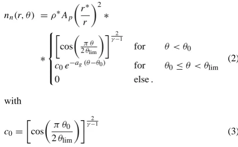
In order to investigate the influence of an anisotropic coma to the larger scale plasma structures a refined model which takes the observed coma anisotropies into account is nec-essary. An anisotropic coma is due to inhomogeneous and localized regions of activity on the cometary surface. Jet-like structures have been found at various comets. In case of 1P/Halley, cometary surface jets have been compared with a gas flow of a rocket exhaustion plume, for which a simple analytical model exists (K¨omle, 1990). This axisymmetric gas-jet model allows us to calculate the neutral gas density as a function of radius r and polar angleθaccording to

nn(r, θ ) =ρ∗Ap

_r∗ r

2

∗

∗

        

cos

π θ

2θlim _γ−2₁

for θ < θ0

c0e−ag(θ−θ0) for θ0≤θ < θlim

0 else.

(2)

with

c0=

cos

_{π θ}

0

2θlim

_γ−2₁

(3)

This model is based on the assumption of a gas flow through a nozzle into vacuum. The continuum flow region is charac-terized by an isentropic core expansion up to a certain angle θ0 and adjacent to it there exists a non-isentropic boundary

layer expansion region up to an angleθlim, as sketched in

Fig. 1. From mass conservation consideration it is possible to derive expressions for the constantsAp,θ0andag. γ is

the adiabatic coefficient of gas, i.e. vapour has 5/3.ρ∗is the nozzle throat gas density andr∗the nozzle throat radius.θlim

is the limiting expansion angle.

lim θ

2 r*

θ₀

Fig. 1. Geometry and model parameters of a supersonic flow from

a reservoir into vaccum (see Eq. 2).

initial particle distributions. On the other hand, observers de-rive, in most cases with a Haser model, integrated outgassing rates from measurements. Since the spatial resolution is lim-ited, it is not possible to localize the gas distribution around the nucleus, so that the information of how the gas is dis-tributed around the nucleus is missing. Therefore, it is rea-sonable to model in all investigated cases an equally active comet for three different geometrical limits.

The neutral gas density for the dayside restricted model reads

nn,2π(r, φ, θ )=α2πnn,4π(r)1[0,π/2)(θ ) . (4)

whereφis the azimuthal angle in the cometocentric coordi-nate system in which the polar axis points in the−x direc-tion. This model is referred to as 2π calculation throughout this paper. The above introduced function 1[0,π )(θ ) is the

indicator function and it is defined according to

1[0,π )(θ ) = (

1 for θ∈ [0, π )

0 else. (5)

The coefficientα2πis derived from the constraint that the

in-tegrated surface activity remains the same for the 2πand 4π cases (see Appendix for more details). Its numerical value is

α2π =2. (6)

For the cone model we restrict the polar angleθaccording to

nn,cπ(r, φ, θ )=αcπnn,4π(r)1[0,π/4)(θ ) . (7)

This model is referred to as cπmodel, with c as an acronym to cone. The calculation ofαcπrelies in complete analogy to

the 2πcase on the constraint that the integrated surface activ-ity remains in thecπcase equal to the 4πcase. Its numerical value is

αcπ =

2 1−1

2

√ 2

≈6.8. (8)

In these coma models spatial confinement leads to an in-crease of the neutral gas density by a factor, which is in case of the dayside Eq. (6) and in case of the cone model Eq. (8). Hence, increasing spatial confinement leads to a rise of the neutral gas density in order to ascertain an equally ac-tive comet.

In Fig. 2 we show a snapshot of the gas cloud through the polar plane of our coordinate system for the three considered test cases. Our coordinate system is defined in Fig. 3. At each time step the code produces pickup currents mass-loading the solar wind according to these three shape models. As in the spherically symmetric limit we assume a neutral gas expansion with a constant outflow velocity on straight lines. From the neutral gas density we infer an ion production rate according to

∂ni(r, φ, θ )

∂t =ν nn(r, φ, θ ) . (9)

It should be mentioned that in this paper we model the coma to consist only of gas. Any dust component is neglected, al-though it has an effect on gas expansion (Keller et al., 1994). The incorporation of a dust component would open a new field of investigation, which at this point would bring us to far away from the topic of interest. Moreover, the current knowledge of gas-dust interaction in the inner coma is a mat-ter of intense research and not yet fully understood.

2.2 Hybrid model

As the applied hybrid simulation code has already been dis-cussed in previous papers (Bagdonat et al., 2002a,b) we re-frain from going into the details of the code. Instead, we briefly present the set up of our simulations.

In the hybrid simulation model a kinetic description of solar wind protons as well as cometary ions is considered. With this method kinetic effects due to the large gyroradii of cometary ions as well as protons compared to the size of the obstacle, which for comets is the spatial extension of the coma, can be studied while retaining a certain amount of efficiency. The spatial coordinate xs and the velocity vs

−15 −10 −5 0 5 10 15

−15 −10 −5 0 5 10 15

z(10

3km)

x(103km)

4 π

−15 −10 −5 0 5 10 15

−15 −10 −5 0 5 10 15

z(10

3km)

x(103km)

2 π

−40 −30 −20 −10 0 10 20 30 40

−40 −30 −20 −10 0 10 20 30 40

z(10

3km)

x(103km)

c π

Fig. 2. Snapshot of the comet outgassing patterns for the three investigated cases at a heliocentric distance of 1.30 AU. At each time step the

hybrid code generates particles according to these patterns. The solar wind enters the box from the left side in +x-direction. On the left we have the spherically symmetric, in the middle the day side restricted and on the right the cone shaped model. We plot the polar plane of our coordinate system. The concentration of particles on the sun illuminated side is clearly visible. Notice the larger scale in the cone shaped model.

d dtxs =vs

d dtvs =

qs

ms

E+vs×B

−kDnn

vs−un

. (10)

Here qs and ms are the charge and mass of a particle of

species s, solar wind protons or cometary ions, respectively; nn and un are the number density and bulk velocity of the

neutrals.kDis a constant describing the collisions of ions and

neutrals, given as 1.7×10−9cm3s−1according to Israelevich et al. (1999).

The electric field equation is derived from a momentum conservation equation of the electron fluid under the as-sumptions of a massless fluid and quasi-neutrality (Bagdo-nat, 2004)

E= −ui×B+

(∇ ×B)×B

µ0ρi

−∇Pe,sw+ ∇Pe,c

ρi

(11) ui is the mean ion bulk velocity andρithe mean ion density.

In this equation two different electron pressure terms have been introduced to account for the substantial difference in the temperatures of electrons of solar wind and cometary ori-gin (Bagdonat, 2004; Boesswetter et al., 2004; Simon et al., 2007). Both electron populations are described by adiabatic laws

Pe,j ∝βe,jnκ_e,j (j =sw, c) . (12)

The condition of quasi-neutrality demands the electron den-sity to equal the ion denden-sityne,j=nj withj=sw, c. A fluid

description of the electrons is justified. Their gyroradius is 0.5 km. This holds for a magnetic field of 4.9 nT and an aver-age velocity of 430 km/s. Thus, their gyroradius is far smaller

Fig. 3. Coordinate system of the three-dimensional simulation. The

electric field E, the magnetic field B and the solar wind velocity v correspond to the undisturbed solar wind conditions. In Sect. 3 we discuss contour plots through thex=0 (terminator), they=0 (polar) and thez=0 (ecliptic) planes.

than the characteristic length scale of the interaction region which is thousands of km large. The plasma betaβe,sw of

solar wind electrons has a value of 0.5 while for electrons of cometary originβe,c is 0.04. In this workκ=2 has been

1560 N. Gortsas et al.: Mapping of coma anisotropies to plasma structures of weak comets

14

N. Gortsas et al.: Mapping of coma anisotropies to plasma structures of weak comets

−15 −10 −5 0 5 10 15

−15 −10 −5 0 5 10 15

z(10

3 km)

x(103km) 4 π

−15 −10 −5 0 5 10 15

−15 −10 −5 0 5 10 15

z(10

3 km)

x(103km) 2 π

−40 −30 −20 −10 0 10 20 30 40

−40 −30 −20 −10 0 10 20 30 40

z(10

3 km)

x(103km) c π

Fig. 2.

Snapshot of the comet outgassing patterns for the three investigated cases at a heliocentric distance of 1.30AU. At each time step the

hybrid code generates particles according to these patterns. The solar wind enters the box from the left side in +x direction. On the left we

have the spherically symmetric, in the middle the day side restricted and on the right the cone shaped model. We plot the polar plane of our

coordinate system. The concentration of particles on the sun illuminated side is clearly visible. Notice the larger scale in the cone shaped

model.

Fig. 3.

Coordinate system of the three dimensional simulation. The

electric field

E

, the magnetic field

B

and the solar wind velocity

v

correspond to the undisturbed solar wind conditions. In section 3

we discuss contour plots through the

x

= 0

(terminator), the

_y

= 0

(polar) and the

z

= 0

(ecliptic) planes.

X Y

Z

Fig. 4.

Snapshot of the three-dimensional calculation at 1.30AU

for the 4

π

case which shows the magnetic field in nT. The drawn

planes are the orthogonal planes of the coordinate axes. The solar

wind enters the box from the left side in +x direction. The

predomi-nant transport of the magnetic field in -z direction is clearly visible.

Furthermore, we discern the formation of a region depleted in the

magnetic field behind the +z-axis. This indicates a low degree of

mixing between the solar wind and cometary species, so that the

magnetic field remains bound to the solar wind flow which leads to

the pileup in front of the obstacle.

Fig. 4. Snapshot of the three-dimensional calculation at 1.30 AU

for the 4π case which shows the magnetic field in nT. The drawn planes are the orthogonal planes of the coordinate axes. The solar wind enters the box from the left side in +x-direction. The pre-dominant transport of the magnetic field in−z-direction is clearly visible. Furthermore, we discern the formation of a region depleted in the magnetic field behind the +z-axis. This indicates a low degree of mixing between the solar wind and cometary species, so that the magnetic field remains bound to the solar wind flow which leads to the pileup in front of the obstacle.

law an equation for the time evolution of the magnetic field is derived (Bagdonat, 2004)

∂B

∂t = ∇ ×(ui×B)− ∇ ×

_{∇ ×B×B}

µ0ρi

. (13)

In Fig. 3 we show the geometry of our 3-D simulation box. The solar wind enters the domain from the −x direction with a constant bulk velocity ub. Upstream we apply

in-flow boundary conditions. Hence, the inserted particles enter the simulation box according to the undisturbed background conditions with a thermal velocity distribution characterized by a width of 25 km/s. Such kind of boundary conditions are applicable since the solar wind flow is supersonic, so that no information from the solar wind-comet interaction trav-els upstream. Downstream we apply outflow boundary con-ditions. Hence, all particles leaving the simulation box are deleted. On the remainder planes we apply inflow bound-ary conditions. We use a Cartesian equidistant grid with a mesh of 90 nodes in each spatial direction. While this res-olution enables us to resolve the inertial length at 3.25 AU, this is no longer true at 1.3 AU. This trade-off is necessary since currently CPU time and memory constraints on current workstations restrict the number of mesh points in each spa-tial direction to around 100.

At the beginning we switch on the comet by producing at each time step a certain amount of particles according

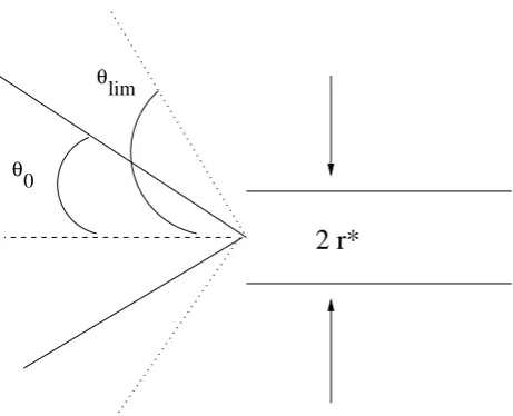
Table 1. Parameters used for the presented simulations.

rH(AU) 1.30 3.25

B0(nT) 4.9 1.6

n0(cm−3) 6.0 0.9

ub(km/s) 430 360

un(km/s) 1 1

Q(s−1) 5×1027 1×1024

N×N×N 90×90×90 90×90×90

βe,sw 0.5 0.5

βe,c 0.04 0.04

ν(s−1) 10−6 10−6

to the discussed shapes (see Fig. 2). Each newly generated cometary macroparticle starts with a constant radial outflow velocity un. Self-consistency is reached after the solar wind

passes several times through the simulation box. The physi-cal parameters of the solar wind plasma have been chosen in accordance to the expected conditions of CG at two different heliocentric distances 3.25 AU (Rosetta instruments on) and 1.30 AU (perihelion) which is in agreement with Hansen et al. (2007). For all three scenarios we use the same values which are summarized in Table 1.

3 Results

The traditional way of presenting 3-D simulation results are 2-D contour plots along cutting planes. Although, this is go-ing to be our method of choice as well we start with a 3-D illustration of the magnetic field at 1.30 AU in Fig. 4. The presentation continues then with Figs. 6, 7 and 8, which show the polar, ecliptic and terminator planes, respectively. In this context Fig. 5 shows 1-D plots along the x-axis. Finally, we present in Fig. 9 the main results of the calculations at 3.25 AU. We chose these two different heliocentric distances because they mark important stages of the Rosetta mission and because they represent two different physical regimes due to the large difference in the activity of the nucleus. In the latter cometary ions serve mainly as test particles while in the former activity is so high that mass loading of the so-lar wind becomes substantial as comparative studies between hybrid and MHD models in Hansen et al. (2007) have shown. Before going into the discussion of the 3-D illustration in Fig. 4 we briefly introduce our coordinate system in Fig. 3. The orthogonal planes of the coordinate axes through the ori-gin of the coordinate system are referred to as terminator, po-lar and ecliptic planes with their orthogonal vector being the x-, y- and z-axis, respectively. Our presentation will be fo-cused on these planes since they provide good insights into the physics of the solar wind-comet interaction.

0.01 0.1 1 10 100 1000

−30 −20 −10 0 10 20 30

n in cm

−3

x in (103 km)

nsw

nhi

(a) _4π

0.01 0.1 1 10 100 1000

−30 −20 −10 0 10 20 30

n in cm

−3

x in (103 km)

nsw

nhi

(b) _2π

0.01 0.1 1 10 100 1000

−30 −20 −10 0 10 20 30

n in cm

−3

x in (103 km)

nsw

nhi

(c) _cπ

0 3 6 9 12 15

−40 −30 −20 −10 0 10 20 30 40

⎪

B

⎪

in nT

x in (103 km)

4π

2π

cπ

(d)

0 100 200 300 400 500

−30 −20 −10 0 10 20 30

⎪

u

⎪

in km/s

x in (103 km)

4π

2π

cπ

(e)

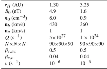
Fig. 5. 1-D plots along the x-axis at 1.30 AU. Panels (a), (b), (c) show the solar wind and the cometary ion density for the three models.

Panels (d), (e) compare the magnetic field and the solar wind bulk velocity for the investigated mass-loading patterns. Due to the high degree of mixing between the species in the cπ case (c) the ICB is only gradually developed. The increase of the mixing region between the two species leads to a broadening of the MBR shown in (d) and a smooth deceleration of the solar wind shown in (e).

spherically symmetric case at 1.30 AU heliocentric distance. A good way to gain access to the wealth of information coded in this presentation is to first discern three distinct different regions. The region in front of the obstacle is characterized by the undisturbed interplanetary magnetic field. Closer to the nucleus the magnetic field is shocked leading to the for-mation of a bow shock (BS) which is accompanied by the magnetic barrier region (MBR) as a parabolic structure from the +z to the−z hemisphere. Behind this structure on the downstream side we recognize a region with reduced values in magnetic field strength. The formation of such a depletion zone is also visible along the terminator and the polar planes of Fig. 4. In regions of an undisturbed solar wind the mag-netic field is transported through convection. However, as the solar wind approaches the nucleus, cometary ion density goes up. In this case mass loading of the solar wind leads to deceleration of the solar wind ions, while the solar wind elec-tron fluid faces an outward directed cometary elecelec-tron pres-sure. Hence, the mixing region of the solar wind species with the cometary species is rather small. Therefore, the magnetic field remains bound to the motion of the solar wind species rather than being passed to the cometary species. This leads to the formation of the MBR with the magnetic field draped around the obstacle.

From now on, we will be solely focused on 2- and 1-D representations of our results. In all contour plots the color scale denotes the strength of the fields while the drawn ar-rows represent the projection of the respective vector fields

on the cutting plane. We are going to focus our discussion on the densities of the solar wind protons and cometary ions, on their respective bulk velocity fields and on the electric as well as the magnetic fields. In order to establish an effi-cient way of reference we introduce the term 4π case for the spherically symmetric case with which we are going to start our discussion. Next we discuss the results of the dayside restricted calculation, which we refer to as 2π run, and in which case we will be particularly interested in differences to the 4π run. In the same manner we will finally present and discuss our findings of the cone shaped run, referred to as cπ case. Since we perform a comparative study with dif-ferent neutral gas sources, we plot in Figs. 6, 7, 8 and 9 all calculated quantities for all runs in three columns as the most efficient way to compare them.

3.1 4πrun at 1.30 AU

0 1 2 3 4 5

x(103km)

(f)⎪E⎪ [V km−1]

z(10 3 km) 16 8 0 −8 −16 16 8 0 −8 −16 0 5 10 15 20 25

(Y)

4

π

2

π

c

π

v_sw

E

(a)n_sw [cm−3]

z(10 3 km) 16 8 0 −8 −16 0 100 200 300 400 500 (b)⎪v_sw⎪ [km s−1]

z(10 3 km) 16 8 0 −8 −16 0.01 0.1 1 10 100 1000 (c)n_hi [cm−3]

z(10 3 km) 16 8 0 −8 −16 0 50 100 150 200 250 (d)⎪v_hi⎪ [km s−1]

z(10 3 km) 16 8 0 −8 −16 0 2 4 6 8 10 12 14

(e)⎪B⎪ [ nT ]

z(10 3 km) 16 8 0 −8 −16 0 1 2 3 4 5

x(103km)

(l)⎪E⎪ [V km−1]

z(10 3 km) 16 8 0 −8 −16 16 8 0 −8 −16 0 5 10 15 20 25 (g)n_sw [cm−3]

z(10 3 km) 16 8 0 −8 −16 0 100 200 300 400 500 (h)⎪v_sw⎪ [km s−1]

z(10 3 km) 16 8 0 −8 −16 0.01 0.1 1 10 100 1000 (i)n_hi [cm−3]

z(10 3 km) 16 8 0 −8 −16 0 50 100 150 200 250 (j)⎪v_hi⎪ [km s−1]

z(10 3 km) 16 8 0 −8 −16 0 2 4 6 8 10 12 14

(k)⎪B⎪ [ nT ]

z(10 3 km) 16 8 0 −8 −16 0 1 2 3 4 5

x(103km)

(r)⎪E⎪ [V km−1]

z(10 3 km) 37 19 0 −19 −37 37 19 0 −19 −37 0 5 10 15 20 25 (m)n_sw [cm−3]

z(10 3 km) 37 19 0 −19 −37 0 100 200 300 400 500 (n)⎪v_sw⎪ [km s−1]

z(10 3 km) 37 19 0 −19 −37 0.01 0.1 1 10 100 1000 (o)n_hi [cm−3]

z(10 3 km) 37 19 0 −19 −37 0 50 100 150 200 250 (p)⎪v_hi⎪ [km s−1]

z(10 3 km) 37 19 0 −19 −37 0 2 4 6 8 10 12 14

(q)⎪B⎪ [ nT ]

z(10 3 km) 37 19 0 −19 −37

Fig. 6. Cut through the polar plane of the simulation box at 1.30 AU. The first column shows the results for the spherically symmetric (4π), the middle column for the day side restricted (2π) and the third column for the cone shaped model (cπ). We show the solar wind density (a,

g, m) and bulk velocity (b, h, n), the cometary ion density (c, i, o) and bulk velocity (d, j, p), the magnetic (e, k, q) and the electric field (f, l, r). The undisturbed solar wind flow points in +x while the convective electric field points in -z direction. Increasing spatial confinment leads

0 1 2 3 4 5

x(103km)

(f)⎪E⎪ [V km−1]

y( 10

3 km )

16 8 0 −8 −16 16 8 0 −8 −16 0 5 10 15 20 25

(Z)

4

π

2

π

c

π

v_sw

B

(a)n_sw [cm−3]

y(10 3 km) 16 8 0 −8 −16 0 100 200 300 400 500 (b)⎪v_sw⎪ [km s−1]

y(10 3 km) 16 8 0 −8 −16 0.01 0.1 1 10 100 1000 (c)n_hi [cm−3]

y(10 3 km) 16 8 0 −8 −16 0 50 100 150 200 250 (d)⎪v_hi⎪ [km s−1]

y(10 3 km) 16 8 0 −8 −16 0 2 4 6 8 10 12 14

(e)⎪B⎪ [ nT ]

y(10 3 km) 16 8 0 −8 −16 0 1 2 3 4 5

x(103km)

(l)⎪E⎪ [V km−1]

y(10 3 km) 16 8 0 −8 −16 16 8 0 −8 −16 0 5 10 15 20 25 (g)n_sw [cm−3]

y(10 3 km) 16 8 0 −8 −16 0 100 200 300 400 500 (h)⎪v_sw⎪ [km s−1]

y(10 3 km) 16 8 0 −8 −16 0.01 0.1 1 10 100 1000 (i)n_hi [cm−3]

y(10 3 km) 16 8 0 −8 −16 0 50 100 150 200 250 (j)⎪v_hi⎪ [km s−1]

y(10 3 km) 16 8 0 −8 −16 0 2 4 6 8 10 12 14

(k)⎪B⎪ [ nT ]

y(10 3 km) 16 8 0 −8 −16 0 1 2 3 4 5

x(103km)

(r)⎪E⎪ [V km−1]

y(10 3 km) 37 19 0 −19 −37 37 19 0 −19 −37 0 5 10 15 20 25 (m)n_sw [cm−3]

y(10 3 km) 37 19 0 −19 −37 0 100 200 300 400 500 (n)⎪v_sw⎪ [km s−1]

y(10 3 km) 37 19 0 −19 −37 0.01 0.1 1 10 100 1000 (o)n_hi [cm−3]

y(10 3 km) 37 19 0 −19 −37 0 50 100 150 200 250 (p)⎪v_hi⎪ [km s−1]

y(10 3 km) 37 19 0 −19 −37 0 2 4 6 8 10 12 14

(q)⎪B⎪ [ nT ]

y(10 3 km) 37 19 0 −19 −37

Fig. 7. Cut through the ecliptic plane of the simulation box at 1.30 AU. Like in Fig. 6 we show from left to right the spherically symmetric,

the day side restricted and the cone shaped model. The solar wind density (a, g, m) and bulk velocity (b, h, n), the cometary ion density (c,

i, o) and bulk velocity (d, j, p), the magnetic (e, k, q) and the electric field (f, l, r) are shown. The undisturbed solar wind flow points in

simulation box a parabolically shaped structure which marks depending on the considered field a transition region with enhanced or decreased magnitudes. The downstream side is characterized by a decrease in magnitude. An obvious rea-son for these common structures is the fact that they are all derived from an equilibrium supersonic background flow. In contrast to that cometary plasma acts as a pollutant, mass loading the solar wind flow. Consequently, cometary proper-ties like density distribution or bulk velocity reveal a distinct different behavior as is visible in Fig. 6c and d.

At a heliocentric distance of 1.30 AU cometary activity of CG is so pronounced that it is in the regime of a fully developed shock as discussed by Bagdonat et al. (2002b). In Fig. 6a we can cleary identify a BS to be located at 4.0×103km from the nucleus along the x-axis. The BS is accompanied by the proton pileup region which exhibits var-ious substructers. These kind of structures have been referred to as shocklets or turbulent structures by Omidi et al. (1990) and they have been observed not only for comets but also for Mars by Boesswetter et al. (2004) and magnetized asteroids by Simon et al. (2006). The characteristic scale of the shock-lets can be derived from the width of the cycloidal motion. A mean velocity of 400 km/s and a magnetic field of 9 nT lead to proton gyroradii of 460 km which in turn leads to a width of the cycloidal motion of 2π rg≈3000 km (Boesswetter et

al., 2004). This value is in good agreement with the width of the BS of about 3500 km along the x-axis.

Another pronounced feature of the BS is its asymmetric structuring along the z-axis, especially visible in Fig. 6a. In the +z hemisphere the density seems to consist several rays while in the−z hemisphere it reaches higher values. Due to the deceleration of solar wind ions and their subsequent ther-malization the individual ion velocity deviates from the back-ground flow. Hence, more solar wind protons are picked-up by the convective electric field which leads to the obsverved predominant particle transport in −z direction. An impor-tant boundary clearly developed in the solar wind density is the ion composition boundary (ICB) or cometopause. This boundary prevents the mixing of the solar wind plasma with the relatively cold cometary ion plasma. Comparing Fig. 6a and c we recognize that in regions of high cometary ion den-sity the solar wind denden-sity is reduced and vice versa. The physical mechanism of this boundary has been investigated for Mars and Titan by Simon et al. (2007). The authors identified a combination of electron pressure and the convec-tive electric field to be responsible for the formation of this boundary. As in principle the discussed mechanism is also applicable on comets, we won’t go into greater details here.

From Fig. 6c we can infer that cometary ions are mainly confined in the tail region. Their motion is predominantly oriented 45◦from the undisturbed solar wind flow in−z di-rection. The heavy cometary ions have large gyroradii caus-ing a motion with large cycloidal arcs. The cometary ion tail to be seen in the−z region of the simulation box is just the first section of this cycloidal arc. With an average velocity of

about 300 km/s and a magnetic field of 5 nT the gyroradius of cometary ions is about 10 000 km. This value has to be com-pared to that part of the tail lying in the simulation box which is of about 16 000 km. The observed cycloidal tail structure correlates very well with the non-vanishing magnetic field downstream of the magnetic barrier region seen in Fig. 6e. This magnetic field is responsible for the gyromotion of the cometary ions visible in Fig. 6c.

The magnetic field in Fig. 6e shows a similar behavior as the solar wind density. Both quantities reach their max-imum values along the x-axis at the same position as shown in Fig. 5a and d. This indicates the excitation of a fast magne-tosonic mode. The MBR is clearly developed and exhibits a spatial width along the x-axis which is larger than the pileup region of the solar wind density. This indicates an increasing degree of mixing between the electron species of solar wind and cometary origin.

The most striking feature of the ecliptic plane shown in Fig. 7 is its symmetry with respect to the x-axis. Since the ecliptic plane is the orthogonal plane of the convective elec-tric field the observed asymmetries along the polar plane are coupled to this field. In Fig. 7a we see the deflection of so-lar wind ions around the obstacle forming two symmetrical lobes. They transport the magnetic field around the obsta-cle as is shown in Fig. 7e. In the terminator plane (Fig. 8) the predominant particle transport of cometary ions and so-lar wind protons is the -z direction. Due to this asymmetry the MBR is not circular but exhibits an asymmetry along the z-axis visible in Fig. 8e.

3.2 2πrun at 1.30 AU

0 1 2 3 4 5

y(103km) (f)⎪E⎪ [V km−1]

z(10 3 km) 16 8 0 −8 −16 16 8 0 −8 −16 0 5 10 15 20 25

(X)

4

π

2

π

c

π

B E

(a)n_sw [cm−3]

z(10 3 km) 16 8 0 −8 −16 0 100 200 300 400 500 (b)⎪v_sw⎪ [km s−1]

z(10 3 km) 16 8 0 −8 −16 0.01 0.1 1 10 100 1000 (c)n_hi [cm−3]

z(10 3 km) 16 8 0 −8 −16 0 50 100 150 200 250 (d)⎪vhi⎪ [km s−1]

z(10 3 km) 16 8 0 −8 −16 0 2 4 6 8 10 12 14

(e)⎪B⎪ [ nT ]

z(10 3 km) 16 8 0 −8 −16 0 1 2 3 4 5

y(103km) (l)⎪E⎪ [V km−1]

z(10 3 km) 16 8 0 −8 −16 16 8 0 −8 −16 0 5 10 15 20 25 (g)n_sw [cm−3]

z(10 3 km) 16 8 0 −8 −16 0 100 200 300 400 500 (h)⎪v_sw⎪ [km s−1]

z(10 3 km) 16 8 0 −8 −16 0.01 0.1 1 10 100 1000 (i)n_hi [cm−3]

z(10 3 km) 16 8 0 −8 −16 0 50 100 150 200 250 (j)⎪vhi⎪ [km s−1]

z(10 3 km) 16 8 0 −8 −16 0 2 4 6 8 10 12 14

(k)⎪B⎪ [ nT ]

z(10 3 km) 16 8 0 −8 −16 0 1 2 3 4 5

y(103km) (r)⎪E⎪ [V km−1]

z(10 3 km) 37 19 0 −19 −37 37 19 0 −19 −37 0 5 10 15 20 25 (m)n_sw [cm−3]

z(10 3 km) 37 19 0 −19 −37 0 100 200 300 400 500 (n)⎪v_sw⎪ [km s−1]

z(10 3 km) 37 19 0 −19 −37 0.01 0.1 1 10 100 1000 (o)n_hi [cm−3]

z(10 3 km) 37 19 0 −19 −37 0 50 100 150 200 250 (p)⎪vhi⎪ [km s−1]

z(10 3 km) 37 19 0 −19 −37 0 2 4 6 8 10 12 14

(q)⎪B⎪ [ nT ]

z(10 3 km) 37 19 0 −19 −37

Fig. 8. Cut through the terminator plane of the simulation box at 1.30 AU. From left to right the results of the spherically symmetric, the day

side restricted and the cone shaped model are shown. The solar wind density (a, g, m) and bulk velocity (b, h, n), the cometary ion density (c,

i, o) and bulk velocity (d, j, p), the magnetic (e, k, q) and the electric field (f, l, r) are the presented quantities. The interplanetary magnetic

0 0.5 1 1.5

x(103km)

(f)⎪E⎪ [V km−1]

z(10 3 km) .3 .2 0 −.2 −.3 .3 .2 0 −.2 −.3 0 1 2 3

(Y)

4

π

2

π

c

π

v_sw

E

(a)n_sw [cm−3]

z(10 3 km) .3 .2 0 −.2 −.3 300 350 400 450 500 (b)⎪v_sw⎪ [km s−1]

z(10 3 km) .3 .2 0 −.2 −.3 0.01 0.1 1 10 100 (c)n_hi [cm−3]

z(10 3 km) .3 .2 0 −.2 −.3 0 50 100 150 (d)⎪v_hi⎪ [km s−1]

z(10 3 km) .3 .2 0 −.2 −.3 0 1 2 3 4

(e)⎪B⎪ [ nT ]

z(10 3 km) .3 .2 0 −.2 −.3 0 0.5 1 1.5

x(103km)

(l)⎪E⎪ [V km−1]

z(10 3 km) .3 .2 0 −.2 −.3 .3 .2 0 −.2 −.3 0 1 2 3 (g)n_sw [cm−3]

z(10 3 km) .3 .2 0 −.2 −.3 300 350 400 450 500 (h)⎪v_sw⎪ [km s−1]

z(10 3 km) .3 .2 0 −.2 −.3 0.01 0.1 1 10 100 (i)n_hi [cm−3]

z(10 3 km) .3 .2 0 −.2 −.3 0 50 100 150 (j)⎪v_hi⎪ [km s−1]

z(10 3 km) .3 .2 0 −.2 −.3 0 1 2 3 4

(k)⎪B⎪ [ nT ]

z(10 3 km) .3 .2 0 −.2 −.3 0 0.5 1 1.5

x(103km)

(r)⎪E⎪ [V km−1]

z(10 3 km) .3 .2 0 −.2 −.3 .3 .2 0 −.2 −.3 0 1 2 3 (m)n_sw [cm−3]

z(10 3 km) .3 .2 0 −.2 −.3 300 350 400 450 500 (n)⎪v_sw⎪ [km s−1]

z(10 3 km) .3 .2 0 −.2 −.3 0.01 0.1 1 10 100 (o)n_hi [cm−3]

z(10 3 km) .3 .2 0 −.2 −.3 0 50 100 150 (p)⎪v_hi⎪ [km s−1]

z(10 3 km) .3 .2 0 −.2 −.3 0 1 2 3 4

(q)⎪B⎪ [ nT ]

z(10 3 km) .3 .2 0 −.2 −.3

Fig. 9. Cut through the polar plane of the simulation box at 3.25 AU. From left to right we show the results for the spherically symmetric,

solar wind proton density and in the magnetic field strength along the x-axis remains comparable to the 4πrun.

The Mach cone of the fast magnetosonic mode exhibits a larger opening angle than in the 4π case. With a mag-netosonic velocity of 300 km/s and of 330 km/s in case of the 4π and 2π runs deduced from Fig. 6b and h we ob-tain an angle between the undisturbed solar wind flow and the fast magnetosonic mode of about 44◦ and 49◦, respec-tively. These values are in good agreement with Fig. 6a and g. The fact that the solar wind density and the magnetic field in Fig. 6g and k exhibit the same behavior clearly indicates the excitation of a fast magnetosonic mode as was the case for the 4π run. Hence, the form of the magnetic barrier re-gion in Fig. 6e and k supports the conclusion of an increased fast magnetosonic wave propagation as a result of the spatial confinement of cometary activity. A comparison of the solar wind density and the magnetic field plots for the two cases in the ecliptic plane Fig. 7a and e, g and k supports the drawn conclusions.

The overall picture of a perceived stronger comet is also confirmed by the solar wind velocity plots in Fig. 6b and h for the 4π and 2π cases, respectively. Since cometary ac-tivity is solely confined to the sun illuminated side of the nucleus mass-loading of the solar wind sets in on a larger distance from the nucleus compared to the 4πrun. However, as Fig. 5e shows the situations remains comparable.

The orientation of the cometary ion tail in Fig. 6i is slightly twisted away from the anti-sunward direction. This indicates an increase of the gyroradius of cometary ions. Taking the magnetic field plot of Fig. 6k into consideration we meet in the downstream side a stronger decrease of the magnetic field, which reduces the cycloidal motion of the cometary ions seen in Fig. 6i. With a magnetic field strength of about 3 nT and an average velocity of about 300 km/s we obtain a gyroradius of the cometary ions of 16 000 km. The gyro-radius has to be compared to the gyrogyro-radius of the 4π run, which is≈10 000 km, and to the extension of the tail lying in the simulation box of about 15 000 km. Since only the beginning of the cycloidal motion is shown in Fig. 6i the pre-dominant transport direction of the cometary ions seems to be twisted away from the sun-comet line. Another visible difference to the 4π case is due to the deployed outgassing pattern. The dayside activity leads to a higher density on the sun illuminated side.

The comparison between the 2π and 4π cases reveals quantitative differences while qualitatively both cases agree well. Therefore, by assuming a spherically symmetric out-gassing comet and by assigning the observed total outout-gassing rate Q also to the nightside of the nucleus one ends up con-sidering a weaker comet. Bagdonat (2004) reported about a similar behavior for a different scenario. By considering a weak comet with the same hybrid code and a spherically symmetric profile, the 4π case of this paper, this investiga-tor observed a similar blow up of the plasma structures by increasing the electron temperature by a factor of 10. In

case of hybrid plasma simulations of Mars Boesswetter et al. (2004) have also confirmed that the electron temperature can modify the observed plasma structures. In this inves-tigation we leave the electron temperature, or the cometary plasma beta, constant for all considered cases. Our aim is to clarify what influence an anisotropic outgassing comet could have on its plasma environment. Therefore, we conclude that in case of small deviations from the spherically symmet-ric outgassing pattern the observed plasma structures show quantitative modifications but qualitatively the overall pic-ture remains the same. The spatial activity pattern of the nu-cleus can quantitatively modify the location and shape of the plasma boundaries encountered at a comet and has to be con-sidered among other parameters, such as the electron temper-ature, in order to fit plasma simulations to observational data. 3.3 cπrun at 1.30 AU

We now switch to the last column of Figs. 6, 7 and 8, which shows the results for the cone shaped model. This outgassing pattern deviates stronger from the spherically symmetric case than the 2π run. Consequently, the observed plasma struc-tures show not only quantitative but also qualitative modifi-cations. An obvious effect of the cone shaped model is the substantial increase of the interaction region. The simulation box has an extension of about 74 000 km twice as large as in the other two cases. A BS is located at a cometocentric position of 18.8×103km as shown in Fig. 6m. Compared to the 4π case this makes an increase of a factor 4.5 which is to some degree comparable to the increase in cometary activity introduced in Eq. (7). The spatial extension of the BS is about 13 600 km along the x-axis which is almost 4 times larger than in the 4π case. The shape of the BS cor-relates to the cone shaped outgassing pattern. It is instruc-tive to take another look at Fig. 2. Similar to the previous two cases we observe in the solar wind the already discussed substructuring of the proton pileup region. The cometary ion tail is to a larger part visible because of the substantially in-creased simulation box. The gyroradius of cometary ions is about 13 000 km for a magnetic field of 3 nT, as deduced from Fig. 6q, and an average velocity of 300 km/s. Hence, some complete cycloidal arcs are included in the simulation box.

that in the cπ case deceleration of the solar wind is much smoother than in the other cases. Hence, the main result of this investigation is that while the solar wind density, shown in Fig. 6m, exhibits similar structures like in the previous two cases, the magnetic field, shown in Fig. 6q, undergoes a distinct different evolution. In addition, the ICB seems to be only gradually developed in contrast to the other cases as inferred from Fig. 5c.

In order to understand this result a quantity4is introduced which relates the width of the mixing regionξ to that of the 4πcase

42π =

ξ(2π )

ξ(4π ). (14)

As a representative value for the width of the mixing region ξ a horizontal line through a density value of 1 cm−3_is

con-sidered reasonable. This mixing ratio4takes a value of 1.4 in case of the 2π run and a value of 4.1 in the cπ model. These figures clearly show that the mixing region between the two species undergoes a slight and a strong increase in case of the dayside and the cone shaped model, respectively. Mass-loading of the solar wind leads to an acceleration of the cometary ions which in turn due to momentum conserva-tion causes a deceleraconserva-tion of the solar wind flow. In case of the cπrun the mass-loaded region is substantially increased. Bearing in mind that at such large distances the gradient of the cometary ion density is rather small, it becomes obvious that mass-loading of the solar wind occurs continuously and not so sharp as in the other cases. Therefore, the solar wind deceleration is smooth. In contrast to that, in the 2πcase the mass-loading region increases but remains with a42π value

of 1.4 comparable to the 4π case. Therefore, the velocity gradient is much steeper than in the cπcase. In addition, the degree of mixing remains weak so that an ICB is clearly de-veloped. That confirms our findings of the previous section and is in good agreement with the respective figures of Fig. 5. However, in case of the cπrun the mixing between the so-lar wind and cometary species, expressed by a mixing ratio 4cπ of 4.1, occurs on a larger scale. Therefore, the ICB is

only gradually established. The large scale mass-loading of the solar wind is also responsible for the broadening of the MBR. The magnetic field is no longer mainly transported by convection through the solar wind species but also with in-creasing intensity through the cometary species. Hence, an additional transport channel of the magnetic field from the barrier region away is established which hampers the peak value and leads to the observed broadening of the magnetic field in Fig. 5d. The cometary bulk velocity plot in Fig. 6p shows that cometary ions reach rather high velocities in the region of 20 000 km which is the position of the MBR. This corroborates the drawn conclusion that the cometary species is increasingly involved in the convective transport of the magnetic field.

The cone shaped model deviates stronger from the spheri-cally symmetric case. It has been studied to simulate a strong

neutral gas jet as observed for many comets. This investiga-tion reveals that increasing spatial confinement leads to an increase of the mass-loaded region along the comet-sun line. This has three effects on the plasma environment of comets. First, the mixing region of solar wind and cometary species is increased which in turn opens an additional transport channel for the magnetic field from the MBR away. Hence, the MBR is broader. Second, this strong mixing leads to a gradually developed ICB. Finally, the deceleration of the solar wind is much smoother than in the previous cases.

3.4 Calculations at 3.25 AU

At a heliocentric distance of 3.25 AU CG is expected to be extremely faint. Therefore, the feedback of cometary activ-ity to the solar wind should be very weak. This expectation is confirmed by the simulation results shown in Fig. 9. In this figure we show the polar plane but the same holds for the terminator and the ecliptic planes which are therefore not shown here.

In the first column of Fig. 9 we show the results for the 4π case. Due to the very faint nucleus the solar wind flow is not altered by the outgassing comet as shown in Fig. 9a and b. The predominant flow direction throughout the simulation box remains the same. Only the magnetic and the electric fields in Fig. 9e and f show first modifications. These are localized and confined to the immediate vicinity of the nu-cleus. The pileup of the magnetic field leads to its increase by almost a factor of 2 compared to the background value. The electric field shows a weak decline in the inner coma. These two configurations should exert according to Eq. (10) a strong force on the solar wind protons but since the cross-section of these modifications is small and the solar wind flow is very fast the interaction time is too short to cause any visible effects on the solar wind flow. The developing twist of the magnetic field excites a fast magnetosonic wave which later on with increasing cometary activity leads to the forma-tion of the linear Mach cone (Bagdonat et al., 2002b). Closer to perihelion this cross-section increases substantially caus-ing the development of different plasma boundaries (see the sections dealing with the 1.30 AU calculations).

The global picture of the cometary ion density shown in Fig. 9c is characterized by the pickup process. The newly born ions expand with an initial velocity of 1 km/s in radial direction. The convective electric and the magnetic fields force the ions on a cycloidal trajectory. Since the spatial ex-tension of the simulation box is 600 km we only encounter the beginning of the cycloidal arc. Assuming a velocity of 50 km/s as indicated by Fig. 9d the gyroradius of the cometary ionsrg,hiis approximately 5200 km. The transport

slightly in the solar wind flow direction. This is clearly vis-ible in the cometary ion density of Fig. 9c. Due to the fi-nite expansion velocity of newly born ions we can discern in Fig. 9c the formation of a so-called heavy ion density jump (HIDJ) (Bagdonat, 2004). The high ion density close to the nucleus is enhanced by deceleration of heavy ions traveling in northward direction and their cycloidal transport in−z di-rection. With increasing cometary activity this HIDJ bound-ary develops into the ICB. For this calculation we can sum-marize that for such low production rates cometary ions serve mainly as test particles despite first modifications of the elec-tromagnetic field topology. This conclusion is in good agree-ment with previous results (Motschmann et al., 2006; Hansen et al., 2007; Bagdonat et al., 2002b).

Switching to the second column of Fig. 9 we can draw the following picture for the dayside restricted case. In analogy to the 4πcase the effects of spatial confinement lead to negli-gible modifications of the solar wind plasma. The solar wind density and velocity field shown in Fig. 9g and h remain un-altered. However, the twist of the magnetic field is here again confined to the inner coma but it is getting stronger as shown in Fig. 9k. Now the jump in magnitude is given by almost a factor of 3. The spatial extension of this modification has increased by roughly a factor of 2. A similar response can be observed in the electric field shown in Fig. 9l. Here, we meet first indications of the formation of a linear Mach cone. In Fig. 9i and j we can recognize the dayside restricted ion cloud. Since at this heliocentric distance the gyroradius of cometary ions is very large the transport of cometary ions in the downstream side is very weak and it occurs mainly in the−z hemisphere. That is the reason for the sharp bound-ary between upstream and downstream, especially in the +z hemisphere. Furthermore, the increasing modifications of the electromagnetic field topology lead to a stronger twist of the cometary ion tail in direction of the undisturbed solar wind flow in comparison to the 4πcase of Fig. 9c.

Finally, switching to the third column of Fig. 9 we can draw the following conclusions about the effects to be ex-pected due to an anisotropic coma morphology. Despite weak cometary activity spatial confinement of newly cre-ated ions lead to stronger modifications in the electromag-netic field topology. In distinction to the 4π and 2π cases we can now observe not only an increase of the magnetic field but also a detachment of it from the inner coma. The center of the twisting magnetic field is now located some 120 km from the nucleus away. It covers an area of about 104km2compared to the 250 km2of the 2π case. The elec-tric field now shows a precursor of a linear Mach cone in the +z direction and adjacent to it in the−z hemisphere a region of almost vanishing field strength. In Fig. 9o and p we can recognize the cone shaped ion cloud. Similar to the 2πcase the observed sharp boundaries in the +z hemisphere are due to the deployed cone shape and the large gyroradius of cometary ions. Furthermore, the increasing modifications of the electromagnetic field topology lead to a stronger twist

of the cometary ion tail in direction of the undisturbed solar wind flow.

4 Summary

In order to address the influence of coma morphology to the plasma environment of comets we have conducted a series of model calculations. Our model regards idealized and sim-plified configurations of real comets. From a gas dynamic model we infer two shape models for the cometary plasma source, a day side restricted and a cone shaped model. For comparison we calculate the widely used spherically sym-metric coma model as well. In order to address two different states of nucleus activity the calculations have been done for two heliocentric distances – 1.30 AU and 3.25 AU. The phys-ical parameters of the calculations have been chosen in accor-dance to the expetected conditions of CG the target comet of the Rosetta mission.

The comparison of the spherically symmetric and the day-side restricted cases reveal a perceived stronger comet in the latter. Spatial confinement of cometary activity on the sun illuminated side of the nucleus leads to a blow up of the plasma structures. The standoff distance of the bow shock and its width along the x-axis are increased by a factor of 1.6, which seems to be correlated to the increase of cometary activity on the dayside by a factor of 2. The opening angle of the Mach cone in the 2π case is increased by a factor of 1.1 compared to the 4π case. The jump of the solar wind den-sity at the ICB and of the magnetic field at the MBR along the x-axis are for both cases almost equal. However, qualita-tively both cases agree very well. Therefore, by assuming a spherically symmetric outgassing comet and by assigning the observed total outgassing rate Q also to the nightside of the nucleus one ends up considering a perceived weaker comet. Therefore we conclude that the spatial activity pattern of the nucleus can quantitatively modify the positions and shapes of the plasma boundaries encountered at a comet and it has to be considered among other parameters, such as the elec-tron temperature (Bagdonat, 2004; Boesswetter et al., 2004), in order to fit plasma simulations to observational data.

Third, it is found that the deceleration of the solar wind is much smoother than in the other two cases.

Our investigations at 3.25 AU confirmed previous results (Motschmann et al., 2006; Hansen et al., 2007; Bagdonat et al., 2002b). The nucleus is so faint that despite spatial confinement almost no modifications of the solar wind flow occurs. For such low production rates cometary ions serve mainly as test particles. Only the electromagnetic field topol-ogy exhibits first modifications. With increasing spatial con-finement the pileup of the magnetic field increases but its cross-section remains too small to cause any visible effects on the solar wind flow. The increased magnetic field leads only to a stronger twist of the cometary ion tail in direction of the solar wind flow. In addition, increasing confinement causes a detachment of the magnetic field pileup region from the immediate vicinity of the nucleus.

Spatial confinement of cometary activity causes visible modifications of the plasma environment of comets. Depend-ing on the deployed mass-loadDepend-ing pattern important plasma structures of comets close to the sun, like the BS, the MBR and the ICB, are modified. Therefore, the actual spatial ac-tivity pattern of the nucleus should be incorporated in plasma simulations of comets. Among other parameters, such as the outgassing rate or the electron temperature the activity pat-tern has to be taken into consideration to interpret observa-tional data. The presented investigation can also be used as a starting point to conduct research on the plasma environment of other bodies in the solar system, known for an anisotropic atmosphere, such as the Saturnian Moon Enceladus.

Appendix A

A key assumption of the presented investigation is that the in-tegrated surface activity remains constant for all three cases. Consider a shell with radial extension of1Rfrom the surface of a spherical nucleus of radiusR0. Let1N denote the

num-ber of particles which are generated during a time interval 1t. The condition of an equally integrated surface activity then reads as

1N4π=1N2π =1Ncπ. (A1)

If the neutral gas densityn(r)is known, the number of parti-cles produced in a time interval1tis obtained from

1N =

Z 2π

0

dφ Z π

0

dθsin(θ )

Z R0+1R R0

dr r2n(r) . (A2)

For the spherical symmetric case given in Eq. (1) this expres-sion evaluates to

1N4π=Q 1t e

−ν R0

un _{. (A3)}

For typical values ofν andun the exponantial evaluates to

almost zero. Hence, the e-term can be set to 1. The time

interval 1t is defined as the time in which a particle trav-els the distance1R with a constant expansion velocityun.

This derivation implies the assumption that the shell is small compared to the nucleus radius1R_R

01. Assume that the

po-lar axis of the cometocentric coordinate system points to the −x direction of the coordinate system in Fig. 3. Then day side activity leads to the following modification of the parti-cle density which is given in Eq. (4)

nn,2π(r)=α2πnn,4π(r)1[0,π/2)(θ ) .

The production of particles is uniform distributed in the angle rangeshφ, θi ∈ [0,2π )×[0, π/2)and obey in radial direc-tion a profile according to ar−2law. The coefficientα2π is

introduced to secure that the integrated activity is equal to the 4πcase. It is obtained from the constraint that the number of particles generated during a time interval1tis in case of the 2π run equal to the 4πcase, which is Eq. (A1). Calculation of the integral in Eq. (A2) yields for the 2πcase

1N2π =

1

2α2πQ 1t e

−ν R0

un _{. (A4)}

Combining this equation with Eqs. (A1) and (A3) yields the following result forα2π

α2π =2. (A5)

In the cone shaped model defined in Eq. (7) the produc-tion of particles is uniform distributed in the angle ranges hφ, θi∈[0,2π )×[0, π/4). In this case, a coefficient αcπ is

introduced to secure that the integrated activity is equal to the 4π case. The neutral gas density of the cone shaped model already given in Eq. (7) reads as

nn,cπ(r)=αcπnn,4π(r)1[0,π/4)(θ ) .

Using Eq. (A2) yields

1Ncπ =2π (1−

1 2

√ 2) 1

4π αcπQ 1t e

−ν R0

un _{. (A6)}

With Eqs. (A1) and (A3) the following value ofαcπ is

ob-tained

αcπ =

2 1−1

2

√ 2

≈6.8. (A7)

Acknowledgements. The work of U. Motschmann, S. Simon and

A. Boesswetter is supported by the Deutsche Forschungsgemein-schaft through grants MO 539/13 and MO 539/15. For Fig. 4 the visualization program developed by Stefan Wiehle, TU Braun-schweig, has been used which is gratefully acknowledged.

Topical Editor I. A. Daglis thanks two anonymous referees for their help in evaluating this paper.

References

Bagdonat, T. and Motschmann, U.: 3D Hybrid Simulation Code Using Curvilinear Coordinates, J. Comput. Physics, 183, 470– 485, 2002.

Bagdonat, T. and Motschmann, U.: From a Weak to a Strong Comet – 3d Global Hybrid Simulation Studies, Earth, Moon and Plan-ets, 90, 305–321, 2002.

Bagdonat, T.: Hybrid Simulation of Weak Comets, PhD Thesis, Technische Universit¨at Braunschweig, 2004.

Benna, M. and Mahaffy, P. R.: New multi-fluid MHD model of comet 26P/Grigg-Skjellerup: Extrapolation to comet 67P/Churyumov-Gerasimenko, Geophys. Res. Lett., 33, 10103, doi:10.1029/2006GL026197, 2006.

Biermann, L., Brosowski, B., and Schmidt, H. U.: The Interaction of the Solar Wind with a Comet, Solar Phys., 1, 254–284, 1967. B¨oßwetter, A., Bagdonat, T., Motschmann, U., and Sauer, K.:

Plasma boundaries at Mars: a 3-D simulation study, Ann. Geo-phys., 22, 4363–4379, 2004,

http://www.ann-geophys.net/22/4363/2004/.

Bogdanov, A., Sauer, K., Baumg¨artel, K., and Srivastava, K. : Plasma structures at weakly outgassing comets-results from bi-ion fluid analysis, Planet. Space Sci., 44, 519–528, 1996. Cochran, A. L.: A re-evaluation of the Haser model scale lengths

for comets, Astron. J., 90, 2609–2614, 1985.

Combi, M. R. and Smyth, W. H.: Monte Carlo particle-trajectory models for neutral cometary gases. I – Models and equations. II – The spatial morphology of the Lyman-alpha coma, Astrophys. J., 327, 1026–1059, 1988.

Combi M. R.: Time-Dependent Gas Kinetics in Tenuous Planetary Atmospheres: The Cometary Coma, Icarus, 123, 207–226, 1996. Combi, M. R., Harris, W. M., and Smyth, W. H.: Gas dynamics and kinetics in the cometary coma: theory and observations, in: Comets II, edited by: Festou, M., Univ. of Arizona Press, 523– 552, 2004.

Delamere, P. A.: Hybrid code simulations of the solar wind inter-action with Comet 19P/Borrelly, J. Geophys. Res., 111, 12217– 12219, 2006.

Feaga, L. M., A’Hearn, M. F., Sunshine, J. M., Groussin, O., and Farnham, T. L.: Asymmetries in the distribution of H2O and CO2 in the inner coma of Comet 9P/Tempel 1 as observed by Deep Impact, Icarus, 190, 345–356, 2007.

Feldman, P. D., Weaver, H. A. and Festou, M. C.: The ultraviolet spectrum of periodic Comet Encke (1980 XI), Icarus, 60, 455– 463, 1984.

Festou, M. C. and Barale, O.: The Asymmetric Coma of Comets. I. Asymmetric Outgassing from the Nucleus of Comet 2P/Encke, Astron. J., 119, 3119–3132, 2000.

Glassmeier, K. H, Boehnhardt, H., Koschny, D., K¨uhrt, E., and Richter, I.: The Rosetta Mission: Flying towards the origin of the solar system, Space Sci. Rev., 128, 1–21, 2007.

Gombosi, T. I., de Zeeuw, D. L., Haberli, R. M., and Powell, K. G.: Three-dimensional multiscale MHD model of cometary plasma environments, J. Geophys. Res., 101, 15233–15254, 1996. Hansen, K. C.,Bagdonat, T.,Motschmann, U., Alexander, C.,

Combi, M. R., Cravens, T. E., Gombosi, T. I., Jia, Y.-D., and Robertson, I. P.: The Plasma Environment of Comet 67P/Churyumov-Gerasimenko Throughout the Rosetta Main Mission, Space Sci. Rev., 128, 133–166, 2007.

Haser, L. and Swings, P.: Sur la possibilit´e d’une fluorescence com´etaire excit´ee par la raie d’´emission Lymanαsolaire,

An-nales d’Astrophysique, 20, 52–52, 1957.

Israelevich, P. L., Gombosi, T. I., Ershkovich, A. I., DeZeeuw, D. L., Neubauer, F. M., and Powell, K. G.: The induced magneto-sphere of comet Halley, 4.: Comparison of in situ observations and numerical simulations, J. Geophys. Res., 104, 28309–28319, 1999.

Jia, Y. D., Combi, M. R., Hansen, K. C., Gombosi, T. I., Crary, F. J., and Young, D. T.: A 3-D Global MHD Model for the effect of neutral jets during the Deep Space 1 comet 19P/Borrelly flyby, Icarus, 196, 249–257, 2008.

Johnstone, A. D., Coates, A. J., Huddleston, D. E., Jockers, K., Wilken, B., Borg, H., Gurgiolo, C., Winningham, J. D., and Am-ata, E.: Observations of the Solar Wind and Cometary Ions dur-ing the Encounter Between Giotto and Comet Grigg-Skjellerup, Astron. Astrophys., 273, 1–4, 1993.

Keller, H. U., Knollenberg, J., and Markiewicz, W. J.: Collima-tion of Cometary Dust Jets and Filaments, Planet. Space Sci., 42, 367–382, 1994.

K¨omle, N. I.: Jet and shell structures in the cometary coma: mod-elling and observations, Comet Halley: Investigations, Results, Interpretations. Vol. 1: Organization, Plasma, Gas, 231–241, 1990.

Lamy, P. L., Toth, I., Weaver, H. A., Jorda, L., Kaasalainen, M., and Guti´errez, P. J.: Hubble Space Telescope observations of the nucleus and inner coma of comet 67P/Churyumov-Gerasimenko, Astron. Astrophys., 458, 669–678, 2006.

Lamy, P. L., Davidsson, B. J. R., Groussin, O., Gutierrez, P., Jorda, L., Kaasalainen, M., and Lowry, S. C.: A Portrait of the Nucleus of Comet 67P/Churyumov-Gerasimenko, Space Sci. Rev., 128, 23–66, 2007.

Lipatov, A. S., Motschmann, U., and Bagdonat, T.: 3D hybrid sim-ulations of the interaction of the solar wind with a weak comet, Planet. Space Sci., 50, 403–411, 2002.

M¨akinen, J. T. T. and Combi, M. R.: Temporal deconvolution of the hydrogen coma I. A hybrid model, Icarus, 177, 217–227, 2005. Mendis, D. A., Houpis, H. L. F., and Marconi, M. L.: The physics

of comets, Fundamentals of Cosmic Physics, 10, 1–4, 1985. Mendis, D. A. and Flammer, K. R.: The Multiple Modes of

Inter-action of the Solar Wind with a Comet as it Approaches the Sun, Earth, Moon and Planets, 31, 301–311, 1984.

Motschmann, U. and K¨uhrt, E.: Interaction of the solar wind with weak obstacles: Hybrid simulations for weakly active comets and for Mars, Space Sci. Rev., 122, 197–208, 2006.

Neubauer, F. M., Marschall, H., Pohl, M., Glassmeier, K.-H., Mus-mann, G., Mariani, F., Acuna, M. H., Burlaga, L. F., Ness, N. F., Wallis, M. K., Schmidt, H. U., and Ungstrup, E.: First results from the Giotto magnetometer experiment during the P/Grigg-Skjellerup encounter, Astron. Astrophys., 268, 5–8, 1993. Neugebauer, M.: Spacecraft observations of the interaction of active

comets with the solar wind, Rev. Geophys., 28, 231–252, 1990. Omidi, N. and Winske, D.: Steepening of kinetic magnetosonic

waves into shocklets: Simulations and consequences for plane-tary shocks and comets, J. Geophys. Res., 95, 2281–2300, 1990. Rauer, H., Helbert, J., Arpigny, C., Benkhoff, J., Bockel´ee-Morvan, D., Boehnhardt, H., Colas, F., Crovisier, J., Hainaut, O., Jorda, L., Kueppers, M., Manfroid, J., and Thomas, N.: Long-term op-tical spectrophotometric monitoring of comet C/1995 O1 (Hale-Bopp), Astron. Astrophys., 397, 1109–1122, 2003.

new target Comet 67P/Churyumov Gerasimenko from narrow-band photometry and imaging, Icarus, 181, 442–457, 2006. Schulz, R. and Schwehm, G.: Coma Composition and Evolution of

Rosetta Target Comet 46P/Wirtanen, Space Sci. Rev., 90, 321– 328, 1999.

Simon, S., Bagdonat, T., Motschmann, U., and Glassmeier, K.-H.: Plasma environment of magnetized asteroids: a 3-D hybrid sim-ulation study, Ann. Geophys., 24, 407–414, 2006,

http://www.ann-geophys.net/24/407/2006/.

Simon, S., Boesswetter, A., Bagdonat, T., and Motschmann, U.: Physics of the Ion Composition Boundary: a comparative 3-D hybrid simulation study of Mars and Titan, Ann. Geophys., 25, 99–115, 2007, http://www.ann-geophys.net/25/99/2007/.

Wegmann, R., Schmidt, H. U. Huebner, W. F., and Boice, D. C.: Cometary MHD and chemistry, Astron. Astrophys, 187, 339– 350, 1987.

Xie, X. and Mumma, M. J.: Monte Carlo Simulation of Cometary Atmospheres: Application to Comet P/Halley at the Time of the Giotto Spacecraft Encounter. II. Axisymmetric Model, As-trophys. J., 464, 457–475, 1996.