www.biogeosciences.net/11/1261/2014/ doi:10.5194/bg-11-1261-2014
© Author(s) 2014. CC Attribution 3.0 License.
Biogeosciences
Technical Note: Approximate Bayesian parameterization of a
process-based tropical forest model
F. Hartig1,2, C. Dislich1,3, T. Wiegand1, and A. Huth1
1UFZ – Helmholtz Centre for Environmental Research, Department of Ecological Modelling, Permoserstr. 15,
04318 Leipzig, Germany
2University of Freiburg, Department of Biometry and Environmental System Analysis, Tennenbacher Str. 4,
79085 Freiburg, Germany
3University of Göttingen, Department of Ecosystem Modelling, Büsgenweg 4,
37077 Göttingen, Germany
Correspondence to: F. Hartig ([email protected])
Received: 28 May 2013 – Published in Biogeosciences Discuss.: 7 August 2013 Revised: 12 January 2014 – Accepted: 17 January 2014 – Published: 27 February 2014
Abstract. Inverse parameter estimation of process-based
models is a long-standing problem in many scientific dis-ciplines. A key question for inverse parameter estimation is how to define the metric that quantifies how well model predictions fit to the data. This metric can be expressed by general cost or objective functions, but statistical inversion methods require a particular metric, the probability of ob-serving the data given the model parameters, known as the likelihood.
For technical and computational reasons, likelihoods for process-based stochastic models are usually based on general assumptions about variability in the observed data, and not on the stochasticity generated by the model. Only in recent years have new methods become available that allow the gen-eration of likelihoods directly from stochastic simulations. Previous applications of these approximate Bayesian meth-ods have concentrated on relatively simple models. Here, we report on the application of a simulation-based likelihood approximation for FORMIND, a parameter-rich individual-based model of tropical forest dynamics.
We show that approximate Bayesian inference, based on a parametric likelihood approximation placed in a conven-tional Markov chain Monte Carlo (MCMC) sampler, per-forms well in retrieving known parameter values from vir-tual inventory data generated by the forest model. We ana-lyze the results of the parameter estimation, examine its sen-sitivity to the choice and aggregation of model outputs and observed data (summary statistics), and demonstrate the
ap-plication of this method by fitting the FORMIND model to field data from an Ecuadorian tropical forest. Finally, we dis-cuss how this approach differs from approximate Bayesian computation (ABC), another method commonly used to gen-erate simulation-based likelihood approximations.
Our results demonstrate that simulation-based inference, which offers considerable conceptual advantages over more traditional methods for inverse parameter estimation, can be successfully applied to process-based models of high com-plexity. The methodology is particularly suitable for hetero-geneous and complex data structures and can easily be ad-justed to other model types, including most stochastic popu-lation and individual-based models. Our study therefore pro-vides a blueprint for a fairly general approach to parameter estimation of stochastic process-based models.
1 Introduction
available (Hartig et al., 2012). These parameters need to be estimated inversely, meaning that they are adjusted by com-paring model outputs to observed data.
To make this comparison, Bayesian methods have become increasingly popular in ecological research during the last decade (e.g., O’Hara et al., 2002; Clark, 2005; Purves et al., 2007; Higgins et al., 2012). In addition to their flexibility and explicit treatment of parameter uncertainty, a particularly ap-pealing property of Bayesian statistics is that they offer the possibility of combining existing information on likely pa-rameters values with the information that is generated in-versely (Hartig et al., 2012). As with other inverse param-eterization approaches, Bayesian methods require the defini-tion of a metric that quantifies how well model predicdefini-tions fit to the observed data. In nonstatistical inversion approaches, such metrics are often called goal functions, objective func-tions or cost funcfunc-tions (e.g., Schröder and Seppelt, 2006). Bayesian approaches use a particular statistical metric, the probability of obtaining the observed data given the current model and parameter values, usually referred to as the likeli-hood.
Most previous applications of Bayesian statistics to process-based ecological models derive this probability by making distributional assumptions about how observations vary around mean model predictions that are independent of the processes in the model, either ad hoc or based on the ob-served variance in the data (e.g., Martínez et al., 2011; van Oijen et al., 2013). This is usually justified with the idea in mind that there is observation uncertainty or variability in en-vironmental conditions that is not accounted for in the model. The approach of constructing likelihoods from such assump-tions is the current state of the art, but it has a major lim-itation: many process-based ecological models are already stochastic and predict variability of certain model outputs. In principle, one would prefer using this variability for deriving the likelihood, because it is based on our mechanistic under-standing of the ecological system and accounts, for exam-ple, for the possibility that expected variability may change with the parameters of the ecological processes. Moreover, once we base our likelihood on the outputs of the stochas-tic model, additional observer submodels that describe how field data were collected could easily be added (e.g., Zurell et al., 2009). However, while theoretically possible, calculat-ing likelihoods for such complicated stochastic interactions used to be intractable in practice (Hartig et al., 2011).
This technical limitation has been reduced in recent years by novel simulation-based approximation techniques that al-low practically any stochastic model to be treated in a for-mal statistical inference framework. Of those, approximate Bayesian computation (ABC; Beaumont, 2010) has arguably attracted most attention, but there are other approaches as well. Their common principle is very simple: what is needed for including a stochastic simulation model in a formal in-ferential framework is the likelihoodp(D|M(φ))for an out-comeDto occur under a modelMwith parametersφ
(Dig-gle and Gratton, 1984). Simulation-based likelihood approx-imations estimate this probability by generating draws from the stochastic model. Subsequently, different methods are used to approximate the likelihood or posterior (Hartig et al., 2011). Often, this involves comparing the model output and observed data by means of data aggregations, also called pat-terns (Wiegand et al., 2004; Grimm and Railsback, 2012) or summary statistics (Beaumont, 2010; Wood, 2010). For brevity, we will refer to these methods in general simply as likelihood approximations, or, in the context of a Bayesian analysis, as approximate Bayesian methods.
The potential of likelihood approximations in ecology has been repeatedly stressed, but applications to community or population ecology are still rare (but see Jabot and Chave, 2009, 2011; May et al., 2013). To our knowledge, there is no previous study that applies likelihood approximations to a computationally expensive, parameter-rich model simulating an ecological community.
The aim of our study is to show that simulation-based like-lihood approximations can be successfully applied to com-plex process-based models. We use a simulation-based like-lihood approximation proposed by Wood (2010) to infer the parameters of FORMIND, an individual-based model of tropical forest communities. We first fit to virtual inventory data that were generated from the model with known param-eters. This allows us to test whether the method can correctly identify all model parameters for different kinds of field data, and to examine how choice and aggregation (summary statis-tics) of data affect the results of the inference. Finally, we ap-ply the method to fit the model to field data from a tropical montane forest in Ecuador.
2 Materials and methods
2.1 Forest gap dynamics and the FORMIND model
Forest ecosystems are locally highly dynamic. One of the most prominent drivers of these dynamics, particularly in the tropics, are natural disturbances, where large trees that have lost stability due to mortality or other factors fall and damage or kill other trees. Gap formation creates a dynamic mosaic of light-filled gaps in natural forests (e.g., Shugart, 1984; McCarthy, 2001). Within these gaps, pioneer species colonize first, until other species take over and continue the successional dynamics that are thought to be one part of the explanation for forest diversity (e.g., Kohyama, 1993).
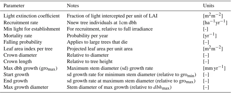
Table 1. Important model parameters and their interpretation. The parameterdbhmaxin the last line refers to the maximum diameter of a
tree, which is a species or PFT-specific parameter of the model (see Dislich et al., 2009).
Parameter Notes Units
Light extinction coefficient Fraction of light intercepted per unit of LAI [m2m−2]
Recruitment rate Nnew tree individuals at 1cm dbh [ha−1yr−1]
Min light for establishment For recruitment, relative to full irradiance [-]
Mortality rate Probability per year [yr−1]
Falling probability Applies to large trees that die [–]
Leaf area index per tree Projected leaf area per unit area [m2m−2]
Crown diameter Relative to diameter [–]
Crown length Relative to tree height [–]
Max dbh growth (gromax) Maximum stem diameter (sd) growth rate [mm yr−1]
Start growth sd growth rate for minimum stem diameter (relative to gromin) [–] End growth sd growth rate at maximum stem diameter (relative to gromax) [–]
Max growth diameter Stem diameter of max growth (relative todbhmax) [–]
functional properties. Parameters and model predictions per plant functional types then represent a mean over the species that are represented by this type. Gap formation by falling dead trees maintains the modeled forest in a dynamic equi-librium. As a result, forest gap models do not merely predict a mean value for outputs such as biomass, species composi-tion, or tree size distributions. Rather, they deliver samples of different possible values for these outputs and therefore allow probabilities to be assigned to different community or biomass states. These predictions of spatiotemporal variation in community composition is what we will use later to derive a probabilistic measure of distance between the model output and observed data.
FORMIND, the forest model used for this study, is a stochastic, individual-based forest model designed in the tra-dition of classical forest gap models (Köhler, 2000). It has been applied for estimating forest succession, variability and disturbances impacts in various tropical locations around the world (e.g., Rüger et al., 2007; Köhler and Huth, 2010; Dis-lich and Huth, 2012; Gutiérrez and Huth, 2012). The sim-ulation area (plot) in FORMIND, which can be of variable size (we use 1 ha throughout the paper) is subdivided into 20 m×20 m grid cells. Tree individuals are assigned to one of these cells and interact with each other on the cell, but do not have an explicit spatial position within the cells. The model state is entirely described by species or functional type, size (measured in diameter at breast height dbh), and location (cell) of all trees. Other variables, such as tree height and crown dimensions, are derived through fixed allometric rela-tionships.
At each time step (we use 5 yr time steps), the light climate in each cell is calculated from the trees on that cell and their respective crowns. Subsequently, establish-ment (light-dependent, stochastic), mortality (stochastic) and tree growth (light-dependent) act on all tree individuals. Important parameters in the model (Table 1) are
recruit-ment and mortality rates, parameters that describe the size-specific maximum growth rates, and the allometric relation-ships that determine height and crown dimensions. Details of these processes, together with a more detailed descrip-tion of the model scheduling, are provided in the Supplement (see also Köhler, 2000; Dislich et al., 2009).
2.2 Bayesian parameter estimation with simulation-based likelihood approximations
We use a Bayesian approach for parameter estimation. One of the advantages of using Bayesian methods with Markov chain Monte Carlo (MCMC) sampling for simulation-based likelihood approximations is that MCMCs, unlike optimiza-tion approaches, are more robust towards variance in likeli-hood estimates generated by the approximation (Hartig et al., 2011). Bayesian methods are also somewhat better suited to dealing with interactions between parameters, which is a phenomenon to be expected in process-based models. In principle, however, one could use the likelihood approxima-tion used in this study with an optimizaapproxima-tion algorithm in a maximum-likelihood framework as well.
There are a number of introductions to Bayesian statistics. A detailed reference is Gelman et al. (2003); for a shorter introduction see Ellison (2004). We give only a brief sum-mary here. The outcome of a Bayesian inference is a proba-bility distributionP (φ|Dobs)for the parametersφgiven the
observed dataDobs. This distribution, called the posterior, is
calculated as
p(φ|Dobs)=c·p(Dobs|M(φ))·p(φ) , (1)
where c is a normalization constant, the prior probability densityp(φ)quantifies parameter uncertainties before com-paring the model to the observed data, and the likelihood functionp(Dobs|M(φ))describes the probability of
Mortality rate [1/yr] of climax type (PFT3)
200 300 400 500 600
Observed biomass Probable
parameter range
0.002 0.004 0.006 0.008
0 2000 4000 6000 8000 10000
0
100
200
300
400
Time [yrs]
Simulated biomass [t/ha]
(a)
Simulated biomass [t/ha]
(b)
100
[image:4.595.85.508.60.274.2]0
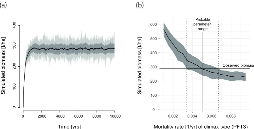
Fig. 1. Principle of statistical inference through stochastic simulation. (a) shows mean model predictions (black), standard deviation (gray)
and min/max values (light gray) for the biomass of a 1 ha plot over 10 000 yr, starting from an empty plot. (b) shows the same mean equilibrium biomass (black) and two standard deviations (gray), but as a function of the mortality of the late-successional type PFT 3; all other parameters constant. Comparing the observed biomass from (a), which was created with a mortality rate of 0.005, with the predicted biomass for different mortality rates, we can infer the original value as well as a statistical uncertainty, without having to define a statistical model.
parametersφ. Broadly speaking, we may say the likelihood quantifies the quality of the fit, while the prior quantifies our prior expectation for each possible parameter value.
Because our main concern in this paper is the approxima-tion of the likelihood, we chose wide uniform (flat) priors for all parameters and data types, which means that the posterior and likelihood are strictly proportional to each other across the possible prior range. Tables with the widths of these uni-form priors are provided in the Supplement. Given that we knew that the model reacts nonlinearly to many parameters, other uninformative prior choices would have been possible (e.g., Kass and Wasserman, 1996), but we felt for the pur-pose of our study it is more useful to ensure proportionality of likelihood and posterior to facilitate the interpretation of the results.
2.2.1 Generating approximate likelihoods
The technical key novelty in this study is the definition of the likelihood p(Dobs|M(φ)). In “conventional” Bayesian
or maximum likelihood studies, this conditional probabil-ity is obtained by formulating an error model that quanti-fies probabilities of deviations between model predictions and observations occurring (e.g., van Oijen et al., 2005). This model may be mechanistically motivated, for example by knowledge about measurement uncertainties. In practi-cal situations, however, there are usually a number of error sources that interact, and error models are therefore typically either fixed ad hoc (van Oijen et al., 2013) or derived from
the observed variability in the data (Martínez et al., 2011). Hence, conventional likelihoods are usually independent of the mechanisms in the process model that is fit.
Our approach goes beyond such an independent error model towards an approach where both the mean model pre-diction and the probability of observing deviations from the mean are derived from the same stochastic ecological cesses. This is particularly promising in systems where pro-cess stochasticity dominates observation errors. For inven-tory data from tropical forests, this is generally the case. Given typical observation errors (see Chave et al., 2004), we can assume that, for small plots, observation uncertainty is small compared to local biomass variation due to succes-sional dynamics (e.g., Chave et al., 2003). FORMIND sim-ulations of the aforementioned successional dynamics trig-gered by gap formation explain the extent of this variability well (e.g., Köhler and Huth, 2010) and can therefore be used to generate statistical expectations for model outputs such as biomass conditional on the model parameters (Fig. 1).
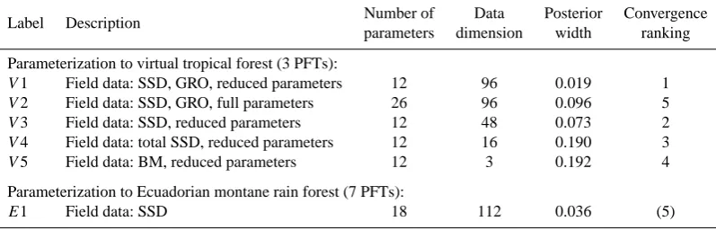
Table 2. Overview of parameter estimations with different models, parameters and summary statistics. Abbreviations for the data: SSD =
stem size distribution (16 10 cm classes); GRO = mean stem diameter growth for each of the 16 10 cm stem diameter classes; BM = biomass. If not stated otherwise, the data type was available for each PFT separately. If we use the mean over all PFTs, we label this “total”. “Full parameters” means that all parameters listed in Tables 1 and 2 of the Supplement are estimated inversely. “Reduced parameters” means that only recruitment, mortality, maximum growth and maximum growth diameter are estimated. “Number of parameters” and “data dimension” give the number of parameters and data points, respectively. “Posterior width” measures the posterior width of the marginal distributions by the ratio between marginal posterior standard deviation and uniform prior width averaged over all parameters. “Convergence ranking” provides a ranking of the speed of convergence of the MCMCs based on the convergence diagnostics discussed in the Supplement. Lower numbers indicate fastest convergence. As E1 uses different data and a different number of PFTs, the convergence ranking is not fully comparable and was set in parentheses.
Label Description Number of Data Posterior Convergence
parameters dimension width ranking
Parameterization to virtual tropical forest (3 PFTs):
V1 Field data: SSD, GRO, reduced parameters 12 96 0.019 1
V2 Field data: SSD, GRO, full parameters 26 96 0.096 5
V3 Field data: SSD, reduced parameters 12 48 0.073 2
V4 Field data: total SSD, reduced parameters 12 16 0.190 3
V5 Field data: BM, reduced parameters 12 3 0.192 4
Parameterization to Ecuadorian montane rain forest (7 PFTs):
E1 Field data: SSD 18 112 0.036 (5)
The principle of this method is to estimatep(Dobs|M(φ)),
for anyφdesired, by fitting a parametric distribution to the output of the stochastic simulation, and estimating the prob-ability of obtainingDobsfrom this distribution (Fig. 2). We
used a multivariate normal distribution because it fitted well to the simulation outputs, and allows a convenient estimation of the covariance structure, but normality is by no means a fundamental requirement of the approach. For the multivari-ate normal approximation, the likelihood of obtaining the ob-served dataDobswith modelMand parametersφis p(Dobs|M(φ))≈c· |6sim(φ)|−1/2exp[−1/2
(Dobs− ¯dsim(φ))T6sim−1(φ)(Dobs− ¯dsim(φ))]. (2)
Here, c=(2π )−k/2, with k being the dimension of Dobs;
¯
dsim(φ)is the corresponding vector of mean simulation
out-puts;6sim(φ)is the covariance matrix of the simulation
out-puts that summarizes variability of and correlations between simulation outputs; and|6sim(φ)| is the determinant of the
covariance matrix. Pseudocode for the entire parameter esti-mation algorithm is provided in the Supplement.
2.2.2 Representation of the data
As in ABC, it is desirable to represent the data used in Eq. (2) in a low-dimensional form so that the estimation particularly of 6−sim1(φ)can be achieved in a computationally efficient way. The challenge here is to find lower-dimensional aggre-gations (summary statistics) of the data that still contain the same amount of information for the purpose of the inference as the raw data (sufficiency). Unfortunately, there is still no
generally accepted rule on how to find good summary statis-tics (but see Fearnhead and Prangle, 2012; Blum et al., 2013). We therefore decided to use mainly two aggregations that have been frequently used for summarizing inventory data in forest modeling, and tested their information content by fitting the model to simulated data. The first aggregation is using stem size distributions, which count the number of tree individuals per (in our study 10 cm) size class per PFT or for all trees. The second is the size-specific mean growth, which quantifies the mean stem diameter growth for different size classes. We also experimented with other forest attributes or aggregations of the data (see Table 2).
2.2.3 Posterior estimation
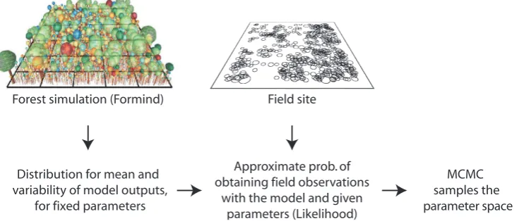
Subsequent posterior estimation based on the approximate likelihood was done with an adaptive Metropolis–Hastings MCMC (Haario et al., 2001). We always ran several chains and checked convergence visually and with Gelman–Rubin diagnostics (Gelman and Rubin, 1992; see Supplement for further details). As several seconds were typically required to evaluate a single parameter combination with FORMIND, posterior estimations cost substantial computing time. The exact number, length and burn-in of chains are provided in the figure captions of the Supplement. Figure 2 provides a visual summary of the analysis method.
2.3 Field data, model setup and analysis
Forest simulation (Formind) Field site
Distribution for mean and variability of model outputs,
for fixed parameters
Approximate prob. of obtaining field observations
with the model and given parameters (Likelihood)
[image:6.595.118.486.67.224.2]MCMC samples the parameter space
Fig. 2. Illustration of the estimation process: at the top left, a visualization representing the FORMIND model. Different colors represent
different PFTs. The model is compared to the field data (middle) by fitting a distribution to the stochastic model output, and calculating the approximate probability of observing the field data from this distribution. This approximate likelihood value feeds into the conventional Bayesian analysis.
successional) that was created from the FORMIND model itself (which has the advantage that the “true” parameter val-ues are known), and a 5 ha forest inventory from a montane tropical rainforest in Ecuador that is described in Dislich et al. (2009). The purpose of the virtual data set is to test the parameter estimation method for different data types in a sit-uation where true parameters are known, while the data from Ecuador provide a realistic case study that allows us to test the method in a situation that had previously been dealt with by manual calibration based on visual assessment of model fit.
To create the virtual inventory, we used a base parameter-ization that was adjusted for exhibiting biomass values and successional patterns typical to a wet tropical lowland rain-forest. With this setting, we simulated 1000 model runs, and created virtual data sets from the mean equilibrium values of these replicates for different types of output variables (sum-mary statistics) such as biomass, stem diameter growth rates and stem size distributions. We also experimented with a dif-ferent number of parameters to be estimated. A summary of these options, labeled V1–V5, is provided in Table 2. For complex models, it can usually not be known a priori which data types are sufficient for a particular inferential question, and we therefore have to test this with virtual data (see also Jabot and Chave, 2009). The number of estimated parame-ters, on the other hand, is more a practical issue: from our understanding of the processes, it was foreseeable that FOR-MIND would exhibit interactions between parameters with respect to these outputs, but it is of practical interest to deter-mine to which extent posterior estimation is slowed down by these interactions, and how those interactions look exactly.
For fitting the model to field data in Ecuador, a tree-species grouping into seven PFTs was used that is described in de-tail in Dislich et al. (2009). Due to data availability, we used
only the stem size distributions for the parameter estimation, which we label E1.
3 Results
3.1 Fit to virtual inventory data (tropical lowland rainforest, V1–V5)
As explained above, we considered a number of options to fit the model to the virtual inventory data. Those options dif-fered in the aggregation of model outputs, and in the number of estimated parameters. We concentrate here on the case V1 in Table 2 (detailed data, not all parameters under calibra-tion). Results for the other cases are discussed in brief below. Detailed results are provided in the Supplement.
3.1.1 Marginal distributions
recruitment_rate_pft1
0.38 0.36 0.86 0.23 0.035
recruitment_rate_pft2
0.40 0.33 0.70 0.14
recruitment_rate_pft3
0.26 0.14 0.40
mortality_pft1
0.28 0.095
mortality_pft2 0.26
mortality_pft3
−0.5 0.0 0.5 1.0
max growth diameter pft3 max growth diameter pft2 max growth diameter pft1 max dbh growth pf3 max dbh growth pf2 max dbh growth pf1 mortality rate pft3 mortality rate pft2 mortality rate pft1 recruitment rate pft3 recruitment rate pft2 recruitment rate pft1
(b)
(a) Marginal parameter distributions of p(φ|D)
Relative difference to the „true“ parameter value
recr1
mort3 mort2 mort1
mort2 mort1 recr3
recr2 recr1 recr3 recr2
mort3
Correlations between parameter in p(φ|D)
• • • • • •
[image:7.595.57.540.59.315.2]• • • • • •
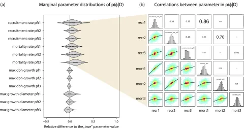
Fig. 3. Summaries of the estimated parameter values (shown as probability distributions) after fitting the model to the virtual inventory data
(case V1 in Table 2). The distributions in (a) correspond to the marginal posterior densityp(φ|D)for each parameter, scaled relative to the “true” values that were used to create the synthetic data (see Table 2 in the Supplement for true values and units). The dot within each distribution denotes the median value. Panels in (b) visualize correlations between recruitment and mortality parameters in the posterior sample (recr1 refers to the recruitment rate of PFT1, mort2 refers to mortality of PFT2 and so on). The diagonal shows the marginal distributions displayed in panel (a). The lower triangle shows the correlation density between the parameters on the diagonal (red values denoting higher density) and a nonlinear fit of the correlation (black line). The upper triangle shows Spearman’s rank correlation coefficients for the correlations in the lower triangle.
3.1.2 Correlations
Marginal distributions represent a cross-section of the pos-terior sample along one parameter, which neglects poten-tial trade-offs between parameters with respect to the data to which the model is fit. Statistical models are usually designed to avoid such correlations wherever possible. For process-based models, on the other hand, the correspondence to spe-cific biological mechanisms is usually the main design crite-rion. It is therefore likely that such correlations will appear when estimating their parameters, as evidenced by Fig. 3b. Moreover, it is to be expected that the correlation structure depends on the data used to fit the model. Less informative data will typically lead to more parameter combinations that can reproduce this data, affecting the correlation structure in the posterior sample.
These expectations are largely confirmed by our results. We find strong positive correlations particularly for recruit-ment and mortality of early successional types, as one would expect, because, for those PFTs, increased mortality can be compensated for to some extent by increased recruitment. Also, we find that the correlation structure changes with the data types used. A detailed analysis of the correlation
struc-ture for the different data types (summary statistics) tested by us is provided in the Supplement.
3.1.3 Choice of data type and number of fitted parameters
0 100 200 300 Posterior predictive
uncertainty Prior predictive uncertainty Uncertainty (due to stoch-asticity) for the true parameter
Predictive uncertainties for the biomass of 1 ha of forest
Biomass [t/ha]
[image:8.595.46.288.86.246.2]400
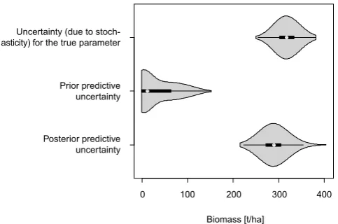
Fig. 4. True, prior and posterior predictive uncertainty. Each
dis-tribution is created from 1000 model runs, observing the biomass on a 1 ha forest plot after 2000 years. The upper distribution shows biomass values from model runs with the same, “true” parameters (Table 2, Supplement), and thereby gives an estimate of the stochas-tic uncertainty of the model. For the middle distribution, model pa-rameters were drawn from the prior distribution (resulting in what is called the prior predictive distribution). For the lower distribution, model parameters were drawn from the posterior (posterior predic-tive uncertainty).
3.1.4 Reduction of predictive uncertainty
The Bayesian framework also allows convenient estimation of the predictive uncertainty before and after fitting the model to the data. We compare three cases, the inherent stochas-tic uncertainty of the model with the true parameters, the uncertainty resulting from parameters drawn from the prior distribution (i.e., before parameter estimation), and the un-certainty for parameters drawn from the posterior distribu-tion (i.e., after parameter estimadistribu-tion). The results displayed in Fig. 4 show that the posterior predictive mean is simi-lar to that of the true parameters, with predictive uncertainty only slightly larger than for the true, fixed parameter value, which indicates that, for a single 1 ha plot, the output uncer-tainty generated from process stochasticity is on the same or-der of magnitude as the uncertainty originating from the pa-rameters. The prior predictive distribution, showing the pre-dictions before calibration, is biased towards smaller values. This is likely due to the fact that many parameters in the prior distribution, in particular those with high mortality, result in very low biomass values.
3.2 Fit to Ecuadorian montane rain forest, E1
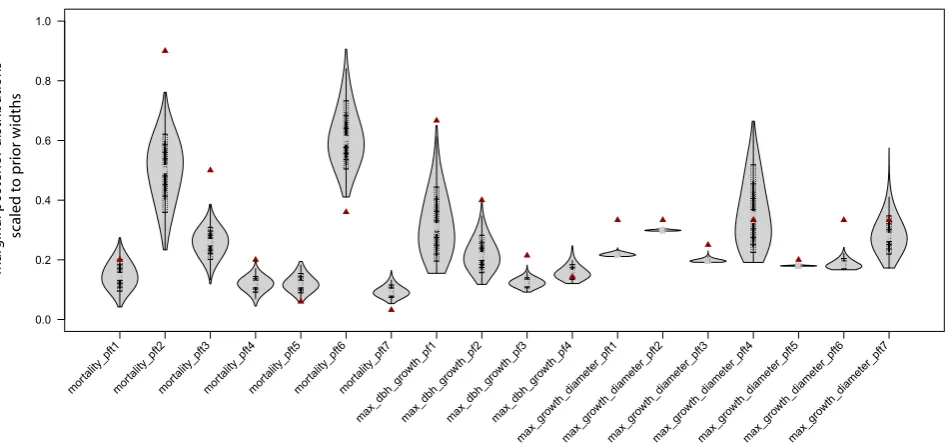
The results of the fit to field data from Ecuador (case E1 in Table 2) are displayed in Fig. 5. We show the marginal dis-tributions for each parameter scaled to the prior range. Pri-ors were uniform distributions within plausible ranges for a
forest of that type. Hence, the figure provides a visual esti-mate of the reduction of parameter uncertainty that would be reached starting from a state at which no specific information about the plot is available. A distribution of a width 0.2, for example, would indicate that the prior uncertainty is reduced by 80 % with the chosen data type. Parameter correlations and unscaled marginal parameter estimates are provided in the Supplement, Figs. 13 and 12, respectively.
4 Discussion
Inverse parameter estimation of ecological models requires a metric that quantifies how well model predictions fit to observed data. Because of technical limitations, the current state of the art is choosing these metrics from expert knowl-edge or deriving them from field data. However, new sta-tistical methods make it possible to generate goodness-of-fit metrics directly from any stochastic simulation model. More specifically, simulation-based likelihood approximations al-low the generation of approximate likelihood functions that return the probability of obtaining a certain field observa-tion given the model parameters directly from the stochastic model outputs. This technique provides a universal and un-ambiguous way to connect stochastic ecological models to field data.
The present study is one of the first to apply this method to a parameter-rich ecological model. We use a parametric like-lihood approximation, proposed by Wood (2010), for fitting FORMIND, a relatively complex individual-based forest gap model, to a range of different virtual inventory data created from the model as well as to real field data from an Ecuado-rian tropical forest.
4.1 Validation of the method with virtual inventory data
pa-mortality_pft1mortality_pft2mortality_pft3mortality_pft4mortality_pft5mortality_pft6mortality_pft7
max_dbh_gro wth_pf1
max_dbh_gro wth_pf2
max_dbh_gro wth_pf3
max_dbh_gro wth_pf4
max_gro wth_diameter_pft1
max_gro wth_diameter_pft2
max_gro
wth_diameter_pft3
max_gro
wth_diameter_pft4
max_gro
wth_diameter_pft5
max_gro
wth_diameter_pft6
max_gro
wth_diameter_pft7
M
ar
g
in
al
p
o
st
er
io
r
d
is
tr
ib
u
ti
o
ns
0.0 0.2 0.4 0.6 0.8 1.0
[image:9.595.63.538.61.284.2]scaled to prior widths
Fig. 5. Marginal posterior probabilities for the model parameters after fitting the model to field data from Ecuador, scaled relative to the
uniform prior distributions (see Table 3 in the Supplement for prior values and units). Values used by Dislich et al. (2009) are marked as dark-red triangles. An unscaled version of these distributions and correlations are provided in Figs. 12 and 13 of the Supplement.
rameter estimates also show correlation between mortality and growth, evidently because growth is unconstrained for this data type.
It is important to take correlations into account when in-terpreting marginal parameter uncertainties such as Fig. 3a: if there are correlations between parameters, marginal un-certainties appear wider than in the multivariate correlation plots. This remains true for higher-order correlations, which are likely present for more aggregated data types used in sce-narios V4 and V5, but which are difficult to visualize. Com-paring the extent to which model parameters are constrained by the data based only on the width of their marginal poste-rior distribution can therefore be misleading in the presence of strong correlations. It is an advantage of the Bayesian anal-ysis (or rather the use of an MCMC) that these interactions can be made explicit and interpreted. Thinking about the rea-sons for correlations may also be helpful for understanding and improving the model structure, although we stress that a correlation in the posterior does not necessarily mean that a parameter is redundant. It merely means that changes in one of the parameters may be counterbalanced by the other to maintain the same value of the model output under consider-ation. For example, correlations and bias increase from V1 to V3, indicating that even for fitting recruitment, mortality and growth parameters only, static data such as stem size distri-butions do not provide sufficient information to constrain all parameters at once. Thus, correlations are connected to a par-ticular data type, and they inform us as to which parameters cannot be fully constraint by this data type.
Bias and correlations observed in the scenarios V1–V5 us-ing the virtual inventory data seemed to originate predomi-nantly from data limitations and not from problems with the simulation-based likelihood approximation. We saw no indi-cations that would suggest that the parametric model (multi-variate normal) used in the likelihood approximation created any problems or bias by not adequately summarizing model outputs, which would be theoretically possible. However, due to the computational complexity of our study, it was not pos-sible to make a more systematic analysis of this question, for example by using virtual replicates of the field data sets or less aggregated data types.
4.2 Fit to Ecuadorian field data
Only static data were available to us for fitting the FOR-MIND model to field data from a montane forest in Ecuador. Our previous analysis suggested that these data would not be sufficient to sensibly constrain all demographic param-eters at once. To get ecologically interpretable results, we therefore fixed the recruitment parameters to the values used in Dislich et al. (2009), and calibrated mortality and growth parameters only. Prior uncertainty was considerably reduced by these data (Fig. 5), suggesting that our approach together with the Ecuadorian data is able to substantially constrain the parameters under calibration. Marginal posterior parameter estimates are similar to those derived by Dislich et al. (2009) with a combination of literature data, expert knowledge and calibration (see Supplement, Table 3 for exact values).
mostly to occur between parameters of the same PFT. We find those correlations, but we also find additional correlations, particularly between the mortality parame-ters of some PFTs (Fig. 13, Supplement). To understand this, one has to know that species grouping designed by Dislich et al. (2009) is hierarchical, consisting of 7 PFTs that were further divided into 4 growth groups with equal maxi-mum diameter growth for the PFTs in each group, with the following relation between (PFT) and growth group: (1)–2, (2)–1, (3,4)–3, and (5,6,7)–4. Diameter growth parameter 3, which is estimated lower, thus applies to the midsuccessional PFTs 3 and 4, and diameter growth parameter 4, estimated higher, applies to the late successional PFTs 5, 6 and 7. This hierarchical species grouping is mirrored in the correlation structure, with particularly strong correlations in the mortal-ity parameters of PFTs that belong to the same growth group. Our interpretation of this pattern is that PFTs in the same growth group are competing more strongly with each other than those that are in different growth groups.
Differences to the parameterization of Dislich et al. (2009) are particularly evident in the mortality parameters. Lower values were estimated for the mortality of the midsucces-sional PFTs 3 and 4, while mortality of the late succesmidsucces-sional PFTs 5, 6 and 7 was estimated higher. This pattern is mir-rored in the maximum diameter growth rates of midsucces-sional species. Thus, our study points to less pronounced differences between mid- and late-successional types than Dislich et al. (2009). We can only speculate about the rea-son for these differences. In general, one would think that the systematic parameter estimation is more reliable than the manual calibration by Dislich et al. (2009). However, although Dislich et al. (2009) calibrated to the same data, they also considered the fit of other model outputs such as total biomass and expert opinions for fixing the param-eters. Expert opinion in particular would favor more pro-nounced differences in mortality rates between mid- and late-successional species due to ecological expectations, al-though specific empirical data on tree mortality or on max-imum growth rates under full light were not available. Sec-ondly, there are significant correlations between the param-eters, which allow us to gain a similar fit with a range of different parameter values. And finally, we were using the model in this study at a lower temporal resolution (5 yr time steps) than Dislich et al. (2009) to reduce computing time, which can affect model dynamics and equilibrium distribu-tions, meaning that slightly different parameter values would be estimated for the same model with different temporal res-olution.
4.3 Advantages compared to conventional calibration methods
Our results demonstrate that inverse parameter estimation with a likelihood function derived from the stochasticity in the model outputs is feasible and provides good results, even
for a relatively complex and runtime-intensive ecological model. This is encouraging in itself, as it is neither trivial to calibrate a parameter-rich model with heterogeneous data in general, nor easy to address all the technical challenges for performing the simulation-based likelihood approximation. A valid question, however, is whether the gain is worth the effort – after all, our approach is connected with consider-able computational and conceptual costs, and all we gain are parameter estimates that could probably also have been de-rived with conventional inversion methods such as parameter optimization.
We believe the effort is justified, particularly because there are practical advantages of simulation-based likelihood ap-proximations for ecological research that extend far beyond what we could demonstrate in this study. First of all, there is considerable interest in connecting models to large and het-erogeneous data sources that become increasingly available (Luo et al., 2011; Hartig et al., 2012; Dietze et al., 2013). A practical problem in this context is that conventional meth-ods provide no good answer as to how different data sources should be weighted to construct a joint likelihood or ob-jective function. Moreover, ecological processes almost in-evitably lead to correlations between those different data types, meaning that we would not expect errors to be in-dependent, posing a challenge for conventional methods. Simulation-based likelihood approximations provide a nat-ural answer to these problems. Assuming that the simulation model includes all major sources of stochasticity, likelihoods approximations automatically weight the importance of dif-ferent model outputs and account for correlations between them. In our study, we can see this in the combined fit of growth rates and stem size distributions, which required no weighting of these two patterns and automatically accounted for correlations between them.
Moreover, under conventional inverse parameterization procedures, one might see that a certain pattern is not well represented, but it is often difficult to decide whether this is a random or a systematic problem. Simulation-based likeli-hood approximations allow us to make a definite statement about the probability of observed patterns given the current model (parameters). Thus, we can use the full arsenal of sta-tistical procedures, including Bayesian and frequentist model selection, to compare alternative ecological hypotheses. The possibility of such rigorous statistical tests for alternative process-based models will likely increase the acceptance of process-based models as a tool, not only for representing and predicting but also for statistically testing ecological knowl-edge.
4.4 Differences to ABC
the more widely used nonparametric approximation used in ABC (Beaumont, 2010). As discussed in Hartig et al. (2011), unlike ABC, parametric likelihood approximations will al-most inevitably exhibit a certain amount of bias because it is unlikely that a simple distributional model can emulate model output distributions in all respects (particularly in the tails of the output distribution). Yet, the parametric approxi-mation also has practical advantages. Many ecological mod-els have to be run into equilibrium before predictions can be made. Once such a model is in equilibrium, more draws for the parametric approximation can be generated relatively cheaply, while a new run has to be started for each ABC step. In our example, the time required for the parametric approx-imation in one MCMC step was not much longer than for an ABC step, but the parametric approximation ensures a good acceptance probability. To reach the same acceptance proba-bility with ABC, we would have to accept a relatively large ABC approximation error. This error may be corrected later, but the fact remains that, for situations where the number of possible MCMC evaluation is fixed (complex models), both ABC and parametric approximations will have a nonnegli-gible error. We conjecture that the balance could well be in favor of parametric approximations in situations such as the one encountered in this study.
5 Conclusions
Our results suggest that likelihood approximations, in partic-ular parametric likelihood approximations, are a promising route for the parameterization of stochastic ecological mod-els. Their use is technically more challenging than the “tra-ditional” Bayesian approach where likelihoods are based on phenomenological error models. The advantage, however, is that error models are based on the same ecological mecha-nisms as all other model predictions. Thus, they allow a more rigorous test of the mechanistic model assumptions, because the mechanisms have to explain both the mean and the vari-ance in the data. Moreover, likelihood approximations ac-count for the relative importance and correlations between different data types predicted by the model, which makes them interesting when models have to be coupled to hetero-geneous data. In this study, additional computational costs of the approach were moderate (factor 2–5) compared to a stan-dard Bayesian approach due to the fact that the model had to be run into equilibrium in any case. Such runtime differ-ences appear secondary compared to the methodological ad-vantage of rigorously testing our mechanistic understanding of ecosystems against field data, including the sampling and measurement process. Parametric likelihood approximations therefore seem particularly promising for models that have to be run into equilibrium, contain the dominant stochastic processes, use heterogeneous data, and predict outputs that can be well summarized by standard distributions.
Supplementary material related to this article is available online at http://www.biogeosciences.net/11/ 1261/2014/bg-11-1261-2014-supplement.pdf.
Acknowledgements. We would like to thank Anja Rammig, Christopher Reyer and Susanne Rolinski for their helpful comments during the review process, and Anne Carney for proofreading. FH acknowledges support from ERC advanced grant 233066. C. Dislich was supported by the German Research Foundation (DFG, Research Unit 816).
The service charges for this open access publication have been covered by a Research Centre of the Helmholtz Association.
Edited by: A. Rammig
References
Beaumont, M. A.: Approximate Bayesian computation in evolution and ecology, Annu. Rev. Ecol. Evol. Syst., 41, 379–406, 2010. Blum, M. G. B., Nunes, M. A., Prangle, D., and Sisson, S. A.: A
comparative review of dimension reduction methods in approxi-mate Bayesian computation, Stat. Sci., 28, 189–208, 2013. Bossel, H.: Real-structure process description as the basis of
under-standing ecosystems and their development, Ecol. Model., 63, 261–276, 1992.
Bugmann, H. K. M.: A simplified forest model to study species composition along climate gradients, Ecology, 77, 2055–2074, 1996.
Chave, J., Condit, R., Lao, S., Caspersen, J. P., Foster, R. B., and Hubbell, S. P.: Spatial and temporal variation of biomass in a tropical forest: results from a large census plot in Panama, J. Ecol., 91, 240–252, 2003.
Chave, J., Condit, R., Aguilar, S., Hernandez, A., Lao, S., and Perez, R.: Error propagation and scaling for tropical forest biomass es-timates, Phil. Trans. R. Soc. B, 359, 409–420, 2004.
Clark, J. S.: Why environmental scientists are becoming Bayesians, Ecol. Lett., 8, 2–14, 2005.
Csilléry, K., Blum, M. G. B., Gaggiotti, O. E., and François, O.: Approximate Bayesian Computation (ABC) in practice, Trends Ecol. Evol., 25, 410–418, 2010.
Dietze, M. C., Lebauer, D. S., and Kooper, R.: On improving the communication between models and data, Plant Cell Environ., 36, 1575–1585, 2013.
Diggle, P. J. and Gratton, R. J.: Monte Carlo methods of inference for implicit statistical models, J. Roy. Stat. Soc. B Met., 46, 193– 227, 1984.
Dislich, C. and Huth, A.: Modelling the impact of shallow land-slides on forest structure in tropical montane forests, Ecol. Model., 239, 40–53, 2012.
Dislich, C., Günter, S., Homeier, J., Schröder, B., and Huth, A.: Simulating forest dynamics of a tropical montane forest in South Ecuador, Erdkunde, 63, 347–364, 2009.
Fearnhead, P. and Prangle, D.: Constructing summary statistics for approximate Bayesian computation: semi-automatic approx-imate Bayesian computation, J. Roy. Stat. Soc. B Met., 74, 419– 474, 2012.
Gelman, A. and Rubin, D.: Inference from iterative simulation using multiple sequences, Stat. Sci., 7, 457–472, 1992.
Gelman, A., Carlin, J. B., Stern, H. S., and Rubin, D. B.: Bayesian Data Analysis, Chapman and Hall, London, 2nd Edn., 2003. Grimm, V. and Railsback, S. F.: Pattern-oriented modelling: a
“multi-scope” for predictive systems ecology, Phil. Trans. R. Soc. B, 367, 298–310, 2012.
Gutiérrez, A. G. and Huth, A.: Successional stages of primary tem-perate rainforests of Chiloé Island, Chile, Perspect. Plant Ecol. Evol. Syst., 14, 243–256, 2012.
Haario, H., Saksman, E., and Tamminen, J.: An adaptive Metropolis algorithm, Bernoulli, 7, 223–242, 2001.
Hartig, F., Calabrese, J. M., Reineking, B., Wiegand, T., and Huth, A.: Statistical inference for stochastic simulation models - theory and application, Ecol. Lett., 14, 816–827, 2011.
Hartig, F., Dyke, J., Hickler, T., Higgins, S. I., O’Hara, R. B., Scheiter, S., and Huth, A.: Connecting dynamic vegetation mod-els to data - an inverse perspective, J. Biogeogr., 39, 2240–2252, 2012.
Higgins, S. I., O’Hara, R. B., Bykova, O., Cramer, M. D., Chuine, I., Gerstner, E.-M., Hickler, T., Morin, X., Kearney, M. R., Midgley, G. F., and Scheiter, S.: A physiological analogy of the niche for projecting the potential distribution of plants, J. Biogeogr., 39, 2132–2145, 2012.
Huth, A. and Ditzer, T.: Simulation of the growth of a lowland Dipterocarp rain forest with FORMIX3, Ecol. Model., 134, 1– 25, 2000.
Jabot, F. and Chave, J.: Inferring the parameters of the neutral theory of biodiversity using phylogenetic information and implications for tropical forests, Ecol. Lett., 12, 239–248, 2009.
Jabot, F. and Chave, J.: Analyzing Tropical Forest Tree Species Abundance Distributions Using a Nonneutral Model and through Approximate Bayesian Inference, Am. Nat., 178, E37–E47, 2011.
Kass, R. E. and Wasserman, L.: The selection of prior distributions by formal rules., J. Am. Stat. Assoc., 91, 1343–1370, 1996. Kohyama, T.: Size-Structured Tree Populations In Gap-Dynamic
Forest - The Forest Architecture Hypothesis For The Stable Co-existence Of Species, J. Ecol., 81, 131–143, 1993.
Köhler, P.: Modelling anthropogenic impacts on the growth of trop-ical rain forests, Ph.D. thesis, University Kassel, Kassel, 2000. Köhler, P. and Huth, A.: Towards ground-truthing of spaceborne
estimates of above-ground life biomass and leaf area index in tropical rain forests, Biogeosciences, 7, 2531–2543, 2010, http://www.biogeosciences.net/7/2531/2010/.
Luo, Y., Ogle, K., Tucker, C., Fei, S., Gao, C., LaDeau, S., Clark, J. S., and Schimel, D. S.: Ecological forecasting and data assim-ilation in a data-rich era, Ecol. Appl., 21, 1429–1442, 2011.
Martínez, I., Wiegand, T., Camarero, J. J., Batllori, E., and Gutiér-rez, E.: Disentangling the formation of contrasting tree line phys-iognomies combining model selection and Bayesian parameteri-zation for simulation models, Am. Nat., 5, E136–E152, 2011. May, F., Giladi, I., Ristow, M., Ziv, Y., and Jeltsch, F.:
Metacom-munity, mainland-island system or island communities? Assess-ing the regional dynamics of plant communities in a fragmented landscape, Ecography, 36, 842–853, 2013.
McCarthy, J.: Gap dynamics of forest trees: A review with particular attention to boreal forests, Environ. Rev., 9, 1–59, 2001. O’Hara, R. B., Arjas, E., Toivonen, H., and Hanski, I.: Bayesian
analysis of metapopulation data, Ecology, 83, 2408–2415, 2002. Pacala, S. W., Canham, C. D., Saponara, J., Silander, J. A., Kobe, R. K., and Ribbens, E.: Forest Models Defined by Field Measure-ments: Estimation, Error Analysis and Dynamics, Ecol. Monogr., 66, 1–43, 1996.
Purves, D. W., Zavala, M. A., Ogle, K., Prieto, F., and Benayas, J. M. R.: Environmental heterogeneity, bird-mediated directed dis-persal, and oak woodland dynamics in mediterranean spain, Ecol. Monogr., 77, 77–97, 2007.
Rüger, N., Gutiérrez, Á. G., Kissling, W. D., Armesto, J. J., and Huth, A.: Ecological impacts of different harvesting scenarios for temperate evergreen rain forest in southern Chile – a simulation experiment, For. Ecol. Manage., 252, 52–66, 2007.
Schröder, B. and Seppelt, R.: Analysis of pattern-process interac-tions based on landscape models–Overview, general concepts, and methodological issues, Ecol. Model., 199, 505–516, 2006. Shugart, H.: Terrestrial ecosystems in changing environments,
Cambridge University Press, Cambridge, UK, 1998.
Shugart, H. H.: A Theory of Forest Dynamics: The Ecological Im-plications of Forest Succession Models, Springer, New York, USA, New York, 1984.
Van Oijen, M., Rougier, J., and Smith, R.: Bayesian calibration of process-based forest models: bridging the gap between models and data, Tree Physiol., 25, 915–927, 2005.
van Oijen, M., Reyer, C., Bohn, F., Cameron, D., Deckmyn, G., Flechsig, M., Härkönen, S., Hartig, F., Huth, A., Kiviste, A., Lasch, P., Mäkela, A., Mette, T., Minunno, F., and Rammer, W.: Bayesian calibration, comparison and averaging of six forest models, using data from Scots pine stands across Europe, For. Ecol. Manage., 289, 255–268, 2013.
Wiegand, T., Knauer, F., Kaczensky, P., and Naves, J.: Expansion of brown bears (Ursus arctos) into the Eastern alps: a spatially ex-plicit population model, Biodivers. Conserv., 13, 79–114, 2004. Wood, S. N.: Statistical inference for noisy nonlinear ecological
dy-namic systems, Nature, 466, 1102–1104, 2010.