www.biogeosciences.net/13/3051/2016/ doi:10.5194/bg-13-3051-2016
© Author(s) 2016. CC Attribution 3.0 License.
High net CO
2
and CH
4
release at a eutrophic shallow lake on
a formerly drained fen
Daniela Franz1, Franziska Koebsch1, Eric Larmanou1, Jürgen Augustin2, and Torsten Sachs1
1Helmholtz Centre Potsdam, GFZ German Research Centre for Geosciences, Telegrafenberg, 14473 Potsdam, Germany 2Institute for Landscape Biogeochemistry, Leibniz Centre for Agricultural Landscape Research (ZALF),
Eberswalder Str. 84, 15374 Müncheberg, Germany
Correspondence to:Daniela Franz (daniela.franz@gfz-potsdam.de)
Received: 14 December 2015 – Published in Biogeosciences Discuss.: 28 January 2016 Revised: 4 May 2016 – Accepted: 6 May 2016 – Published: 25 May 2016
Abstract. Drained peatlands often act as carbon dioxide (CO2)hotspots. Raising the groundwater table is expected
to reduce their CO2 contribution to the atmosphere and
re-vitalise their function as carbon (C) sink in the long term. Without strict water management rewetting often results in partial flooding and the formation of spatially heterogeneous, nutrient-rich shallow lakes. Uncertainties remain as to when the intended effect of rewetting is achieved, as this spe-cific ecosystem type has hardly been investigated in terms of greenhouse gas (GHG) exchange. In most cases of rewetting, methane (CH4)emissions increase under anoxic conditions
due to a higher water table and in terms of global warming potential (GWP) outperform the shift towards CO2uptake, at
least in the short term.
Based on eddy covariance measurements we studied the ecosystem–atmosphere exchange of CH4and CO2at a
shal-low lake situated on a former fen grassland in northeastern Germany. The lake evolved shortly after flooding, 9 years previous to our investigation period. The ecosystem con-sists of two main surface types: open water (inhabited by submerged and floating vegetation) and emergent vegetation (particularly including the eulittoral zone of the lake, dom-inated byTypha latifolia). To determine the individual con-tribution of the two main surface types to the net CO2and
CH4 exchange of the whole lake ecosystem, we combined
footprint analysis with CH4modelling and net ecosystem
ex-change partitioning.
The CH4and CO2dynamics were strikingly different
be-tween open water and emergent vegetation. Net CH4
emis-sions from the open water area were around 4-fold higher than from emergent vegetation stands, accounting for 53
and 13 g CH4m−2a−1respectively. In addition, both surface
types were net CO2sources with 158 and 750 g CO2m−2a−1
respectively. Unusual meteorological conditions in terms of a warm and dry summer and a mild winter might have fa-cilitated high respiration rates. In sum, even after 9 years of rewetting the lake ecosystem exhibited a considerable C loss and global warming impact, the latter mainly driven by high CH4emissions. We assume the eutrophic conditions in
com-bination with permanent high inundation as major reasons for the unfavourable GHG balance.
1 Introduction
Peatland ecosystems play an important role in global green-house gas (GHG) cycles, although they cover only about 3 % of the earth’s surface (Frolking et al., 2011). Peat growth de-pends on the proportion of carbon (C) sequestration and re-lease. Pristine peatlands act as long-term C sinks and are near neutral (slightly cooling) regarding their global warming po-tential (GWP; Frolking et al., 2011), dependent on rates of C sequestration and methane (CH4)emissions. However, many
2012; Beetz et al., 2013). However, lowering the water ta-ble is typically accompanied with decreasing CH4emissions
(Roulet et al., 1993). Emission factors of 1.6 g CH4m−2a−1
and 2235 g CO2m−2a−1 were assigned to temperate
deep-drained nutrient-rich grassland in the 2013 wetland supple-ment to the 2006 IPCC Guidelines for National Greenhouse Gas Inventories (IPCC, 2014).
In the last decades rewetting of peatlands attracted atten-tion in order to stop soil degradaatten-tion, reduce CO2emissions
and recover their functions as C and nutrient sink and ecolog-ical habitat (Zak et al., 2015). Large rewetting projects were initiated, e.g. the Mire Restoration Program of the federal state of Mecklenburg–West Pomerania in northeastern (NE) Germany (Berg et al., 2000) starting in 2000 and involv-ing 20 000 ha of formerly drained peatlands, especially fens (Zerbe et al., 2013) e.g. in the Peene river catchment. How-ever, uncertainties remain as to when the intended effects of rewetting are achieved. Only a few studies exist on the tem-poral development of GHG emissions of rewetted fens, es-pecially on longer timescales. Augustin and Joosten (2007) discuss three very different states following peatland rewet-ting based on observations at Belarusian mires, though with-out specifying the individual lengths of the phases. Broad agreement exists concerning the CH4hotspot characteristic
of newly rewetted peatlands (e.g. Meyer et al., 2001; Hahn-Schöfl et al., 2011; Knox et al., 2015). However, a rapid re-covery of the net CO2sink function is not consistently
re-ported (e.g. Wilson et al., 2007).
Peatlands develop a distinct microtopography after drainage and subsequent subsidence. Rewetting, e.g. in the Peene river catchment, resulted in the formation of large-scale shallow lakes in the lower parts of the fens, with water depths usually below 1 m (Zak et al., 2015; Steffenhagen et al., 2012). These new ecosystems are nutrient rich and most often strikingly different from natural peatlands. They expe-rience a rapid secondary plant succession (Zak et al., 2015). Helophytes are expected to progressively enter the open wa-ter body over time, leading to the wa-terrestrialisation of the shal-low lake and in the best case peat formation. However, this new ecosystem type and its progressive transformation have hardly been investigated in terms of GHG dynamics. The ecosystem-inherent spatial heterogeneity suggests complex patterns of GHG emissions due to distinct GHG source or sink characteristics of the involved surface types (generally open water and the littoral zone), resulting in measurement challenges. Site-specific heterogeneity implicitly has to be considered for the evaluation of ecosystem-scale flux mea-surements (e.g. Barcza et al., 2009; Hendriks et al., 2010; Herbst et al., 2011; Hatala Matthes et al., 2014). The impor-tance of small open water bodies in wetlands as considerable GHG sources was highlighted in previous studies (e.g. by Schrier-Uijl et al., 2011; Zhu et al., 2012; IPCC, 2014) and in the case of CH4even for landscape-scale budgets (e.g. by
Repo et al., 2007). In addition, the littoral zone of lakes is often found to be a CH4hotspot (Juutinen et al., 2003; Wang
Study site
(a) (b)
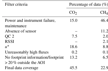
Figure 1. (a)Polder Zarnekow is situated in NE Germany within the Peene river valley; map source and copyright: https://commons. wikimedia.org/wiki/File:Germanymap2.png (modified).(b) Foot-print climatology calculated according to Chen et al. (2011) on a Landsat image (6 June 2013, source: Google Earth). White lines represent the isopleths of the cumulative annual footprint climatol-ogy, where the area within the 95 isopleth indicates 95 % contribu-tion to the annual flux. The white dot denotes the tower posicontribu-tion. The yellow box indicates the area of interest (AOI) as a filter crite-rion to focus on fluxes of the shallow lake and to avoid the possible impact of a farm and grassland to the north of the shallow lake. If the half-hourly flux source area exceeded the AOI by more than 20 % the flux was discarded. The site is characterised by two main surface types: open water and emergent vegetation.
et al., 2006) with a contribution of up to 90 % to the whole-lake CH4release (Smith and Lewis, 1992), albeit depending
on the lake size (Bastviken et al., 2004) and plant commu-nity. Rõõm et al. (2014) measured the largest CH4(and CO2)
emissions of a temperate eutrophic lake at the helophyte zone within the littoral.
The objectives of this study are (1) to investigate the ecosystem–atmosphere exchange of CH4 and CO2 (net
ecosystem exchange, NEE) of a nutrient-rich lake ecosys-tem emerged at a former fen grassland and (2) particularly infer the individual GHG dynamics of the main surface types within the ecosystem and quantify their contribution to the annual exchange rates. Therefore, we applied the eddy co-variance (EC) technique from May 2013 to May 2014 and used an analytical footprint model to downscale the spatially integrated, half-hourly fluxes to the main surface types “open water” and “emergent vegetation”. The resulting source area (i.e. spatial origin of the flux) fractions were then included in a temperature response (CH4)and NEE partitioning model
(CO2)in order to quantify the source strength of the two
[image:2.612.309.548.67.201.2]2 Material and methods 2.1 Study site
The study site “Polder Zarnekow” is a rewetted, rich fen (minerotrophic peatland) located in the Peene river valley (Mecklenburg–West Pomerania, NE Germany, 53◦52.50N 12◦53.30E; see Fig. 1), with less than 0.5 m a.s.l. elevation. It is part of the Terrestrial Environmental Observatories Net-work (TERENO). The temperate climate is characterised by a long-term mean annual air temperature and mean an-nual precipitation of 8.7◦C and 584 mm respectively (Ger-man Weather Service, meteorological station Teterow, 24 km southwest of the study site; reference period 1981–2010). The geomorphological character of the area is predominantly a result of the Weichselian glaciation as the last period of the Pleistocene (Steffenhagen et al., 2012). The fen devel-oped with continuous percolating groundwater flow (Suc-cow, 2001). Peat depth partially reaches 10 m (Hahn-Schöfl et al., 2011). Drainage was initialised in the 18th century and strongly intensified between 1960 and 1990 within an exten-sive melioration program (Höper et al., 2008). The decline of the water table to > 1 m below surface and subsequent de-composition and mineralisation of the peat (especially in the upper 30 cm, Hahn-Schöfl et al., 2011) caused phosphor fer-tilisation (Zak et al., 2008) and soil subsidence to levels be-low that of adjacent freshwater bodies (Steffenhagen et al., 2012; Zerbe et al., 2013). The latter simplified the rewetting process which was initiated in winter 2004/2005 by opening the dikes.
In consequence of flooding the drained fen was converted into a spatially heterogeneous site of emergent vegetation (on temporarily inundated soil) and permanent open water areas. In this study we focus on a eutrophic and polymictic lake (open water body about 7.5 ha) as part of the rewetted area, with water depths ranging from 0.2 to 1.2 m (2004 to 2012; Zak et al., 2015). During the study period the open water body of the lake was inhabited by submerged and floating macrophytes, particularlyCeratophyllum demersum,Lemna
minor, Spirodela polyrhiza (Steffenhagen et al., 2012) and
Polygonum amphibium, which correspond to the sublittoral
zone in a typical lake zonation. CeratophyllumandLemna
sp. were already reported to colonise the lake in the second year of rewetting (Hahn-Schöfl et al., 2011).Phalaris arund-inacea, which dominated the fen before rewetting, died off in the first year of inundation (Hahn-Schöfl et al., 2011) and has been limited to the non-inundated periphery of the ecosys-tem. Helophytes (e.g.Glyceria,Typha) started the colonisa-tion of lake margins and other temporarily inundated areas in the third year of rewetting. The eulittoral zone of the lake is now dominated byTypha latifoliastands gradually colonis-ing the open water in the last years. Emergent vegetation stands also include sedges asCarex gracilis(Steffenhagen et al., 2012). At the bottom of the shallow lake an up to 30 cm thick layer of organic sediment evolved, initially fed by fresh
plant material of the former vegetation and since then contin-uously replenished by recent aquatic plants and helophytes after die-back (Hahn-Schöfl et al., 2011).
2.2 Eddy covariance and additional measurements We conducted EC measurements of CO2and CH4exchange
on a tower placed on a stationary platform at the NE edge of the shallow lake (see Fig. 1). Thereby we ensured to fre-quently catch the signal from both the open water body and
theTypha latifolia dominated belt of the shallow lake
(eu-littoral zone). We defined an area of interest (AOI) in order to focus on an ecosystem dominated by a shallow lake and to avoid a possible impact of the farm and grassland to the north of the shallow lake. The EC measurement setup included an ultrasonic anemometer for the 3-D wind vector (u, v, w) and sonic temperature (HS-50, Gill, Lymington, Hampshire, UK), an enclosed-path infrared gas analyser (IRGA) and an open-path IRGA for CO2/H2O and CH4concentrations
re-spectively (LI-7200 and LI-7700, LI-COR Biogeosciences, Lincoln, NE, USA). Flow rate was about 10–11 L min−1. Measurement height was on average 2.63 m above the water surface at the position of the tower, depending on the wa-ter level. We recorded raw turbulence and concentration data with a LI-7550 digital data logger system (LI-COR Biogeo-sciences, Lincoln, NE, USA) at 20 Hz in half-hourly files. The data set is shown in coordinated universal time (UTC), which is 1 h behind local time.
We further equipped the tower with instrumentation for net radiation, air temperature/humidity, 2-D wind direction and speed, incoming and reflected photosynthetic photon flux density (PPFD/PPFDr) and water level. Additional mea-surements in close proximity to the tower included precipi-tation, soil heat flux as well as soil and water temperature. Soil temperature was measured below the water column in depths of 10, 20, 30, 40 and 50 cm and water temperature at the sediment–water interface. All non-eddy covariance-related measurements were logged as 1 min averages/sums (precipitation). Gaps were filled with measurements of the Leibniz Centre for Agricultural Landscape Research (ZALF, Müncheberg, Germany) at the same platform and a nearby climate station (climate station Karlshof, GFZ German Re-search Centre for Geosciences, 14 km distance from study site; Itzerott, 2015).
A water density gradient was calculated based on the tem-perature at the water surface and at the sediment–water inter-face. The water surface temperature was calculated based on the Stefan–Boltzmann law:
Tw= 4
s
I εwσSB
, (1)
whereTwis the water surface temperature (K),I is the
long-wave outgoing radiation (W m−2),εw is the infrared
emis-sivity of water (0.960) andσSBis the Stefan–Boltzmann
the air-saturated water at the water surface and the sediment– water interface according to Bignell (1983):
ρas=ρaf−0.004612+0.000106·T , (2)
whereρas is the density of the respective air-saturated water
(k m−3), ρaf is the density of the respective air-free water
(k m−3; see Wagner and Pruß, 2002) at atmospheric
pres-sure (1013 hPa) and T is the respective water temperature (◦C). The gradient of the two water densities (air-saturated) 1ρ/1z was calculated as difference of the water density (air-saturated) at the sediment–water interface and the sur-face water density (air-saturated), divided by the distance (m) between the two basic temperature measurements. Changes of the distance due to the fluctuating water level were con-sidered. Positive and negative gradients indicate periods of stratification and thermally induced convective mixing of the water column respectively.
2.3 Flux computation and further processing
For this analysis we used data from 14 May 2013 to 14 May 2014. We calculated half-hourly fluxes of CO2 and
CH4based on the covariances between the respective scalar
concentration and the vertical wind velocity using the pro-cessing package EddyPro 5.2.0 (LI-COR, Lincoln, Nebraska, USA). Sonic temperature was corrected for humidity effects according to van Dijk et al. (2004). Artificial data spikes were removed from the 20 Hz data following Vickers and Mahrt (1997). We used the planar fit method (Finnigan et al., 2003; Wilczak et al., 2001) for axis rotation and defined the sector borders according to Siebicke et al. (2012). Block av-eraging was used to detrend turbulent fluctuations. For time lag compensation we applied covariance maximisation (Fan et al., 1990). Spectral losses due to crosswind and vertical instrument separation were corrected according to Horst and Lenschow (2009). The methods of Moncrieff et al. (2004) and Fratini et al. (2012) were used for the correction of high-pass filtering and low-high-pass filtering effects respectively. For fluctuations of CH4density we corrected changes in air
den-sity according to Webb et al. (1980), considering LI-7700-specific spectroscopic effects (McDermitt et al., 2011). Ac-cording to the micrometeorological sign convention, positive values represent fluxes from the ecosystem into the sphere (emission) and negative values fluxes from the atmo-sphere into the ecosystem (ecosystem uptake).
2.4 Quality assurance
We filtered the averaged fluxes according to their quality as follows (see Table 1, for final measurement data coverage see Fig. A1 in Appendix A).
[image:4.612.313.543.117.267.2]– We rejected fluxes with quality flag 2 (QC 2, bad qual-ity) based on the 0–1–2 system of Mauder and Fo-ken (2004).
Table 1.Data loss and final data coverage during the observation pe-riod. CO2and CH4flux data were lost by power and instrument fail-ure and maintenance as well as quality control and footprint analy-sis.
Filter criteria Percentage of data (%)
CO2 CH4
Power and instrument failure, 15.0 46.4 maintenance
Absence of sensor – 11.2
QC 2 7.5 2.0
RSSI – 2.1
u∗ 18.6 8.8
Unreasonably high fluxes 0.2 0.1
No footprint information/footprint 13.2 6.5 > 20 % outside the AOI
Final data coverage 45.5 22.9
– CH4 fluxes were skipped if the signal strength (RSSI)
was below the threshold of 14 %. This threshold was estimated according to Dengel et al. (2011).
– Fluxes with friction velocity (u∗) < 0.12 and > 0.76 m s−1 were not included due to consider-ably high fluxes beyond these thresholds, which were estimated similar to the procedure described in Aubinet et al. (2012) based on binnedu∗ classes. The storage term was calculated as described in Béziat et al. (2009). – Unreasonably high positive and negative fluxes (0.2 %/99.8 % percentile) were discarded from the CO2
and CH4flux data set.
Quality control (apart from EddyPro internal steps) and the subsequent processing steps were performed with the free software environment R (R Core Team, 2012).
2.5 Footprint modelling
footprint information was not available or more than 20 % of the source area was outside the AOI (see Fig. 1 and Table 1). The fractional coverage within the AOI (Ai)was 21.7 % for
open water.
Quasi-continuous source area information for the two sur-face types was achieved by gap filling the results of the foot-print model with the means of the source area fractions of the surface types (i)for 1◦wind direction intervals, separately
for stable and unstable conditions. In case the sum of the i was less than 100 %, when the source area exceeded the
set borders, we assigned the remaining contribution percent-ages to emergent vegetation, as the area beyond the borders is dominated by emergent vegetation rather than open water. 2.6 Gap filling
A marginal distribution sampling (MDS) approach pro-posed by Reichstein et al. (2005), available as a web tool based on the R package REddyProc (http://www.bgc-jena. mpg.de/REddyProc/brew/REddyProc.rhtml), was applied for gap filling and partitioning of NEE measurements (MDSCO2nofoot), with air temperature as temperature
vari-able. For the gap filling of CH4measurements non-linear
re-gression (NLR) was applied (NLRCH4nofoot):
FCH4=exp(a+b1·X1+. . .+bj·Xj), (3)
wherea andb1. . .bj are fitting parameters andX1. . .Xj are
environmental parameters. Several environmental parame-ters, which were reported to be correlated with CH4flux on
different timescales, were tested to find the best bi- or mul-tivariate NLR model for the ecosystem CH4 flux: pressure
change, u∗, PAR, air temperature, soil heat flux, soil/peat temperature in different heights and water level. Only fluxes of the best quality (QC 0) were used to fit the NLR model and the MDS.
2.7 Calculation of the annual CO2and CH4budget and the global warming potential
We used the continuous flux data sets derived from gap fill-ing for the calculation of annual CO2and CH4budgets. The
ecosystem GHG balance was calculated by summation of the NEE of CO2 and CH4 using the GWP of each gas at the
100-year time horizon (IPCC, 2013). According to the IPCC AR5 (IPCC, 2013) CH4has a 28-fold global warming
poten-tial compared to CO2(without inclusion of climate–carbon
feedbacks).
The uncertainty of the annual estimates was calculated as the square root of the sum of the squared random error (mea-surement uncertainty) and gap-filling error within the 1-year observation period (see e.g. Hommeltenberg et al., 2014; Shoemaker et al., 2015). An estimation of the random un-certainty due to the stochastic nature of turbulent sampling according to Finkelstein and Sims (2001) is implemented in EddyPro 5.2.0. In case of the MDS approach the gap-filling
error (standard error) was calculated from the standard devi-ation of the fluxes used for gap filling, provided by the web tool. For budgets based on the NLR approach we used the residual standard error of the NLR model as gap-filling error (following Shoemaker et al., 2015).
2.8 Estimation of surface type fluxes
To estimate the specific surface type fluxes, we combined footprint analysis with NEE partitioning (using NLR) to as-sign gross primary production (GPP) and ecosystem respira-tion (Reco)to the two main surface types (NLRCO2foot).Reco
and GPP were modelled as sum of the two surface type fluxes weighted byi (analogous to Forbrich et al., 2011).
Night-timeReco (global radiation < 10 W m−2)was estimated by
the exponential temperature response model of Lloyd and Taylor (1994) assuming that night-time NEE represents the night-timeReco:
Reco=
2
X
i=1
i·Rrefi·exp
E0i
1
Tref−T0
− 1
Tair−T0
, (4) whereReco is the half-hourly measured ecosystem
respira-tion (µmol−1m−2s−1),i is the source area fraction of the
respective surface type,Rrefis the respiration rate at the
refer-ence temperatureTref(283.15 K),E0defines the temperature
sensitivity,T0is the starting temperature constant (227.13 K)
andTair the mean air temperature during the flux
measure-ment. The model parameters achieved for night-time Reco
were applied for the modelling of daytime Reco. GPP was
calculated by subtracting daytimeReco from the measured
NEE. GPP was further modelled using a rectangular, hyper-bolic light response equation based on the Michaelis–Menten kinetic (see e.g. Falge et al., 2001):
GPP= 2
X
i=1
i·
GP
maxi·αi·PAR
αi·PAR+GPmaxi
, (5)
where GPP is the calculated gross primary production (µmol−1m−2s−1),i is the source area fraction of the
re-spective surface type, GPmax is the maximum C fixation
rate at infinite photon flux density of the photosynthetic ac-tive radiation PAR (µmol−1m−2s−1)andαis the light use efficiency (mol CO2mol−1photons). We calculated one
pa-rameter set for Reco and GPP per day based on a moving
window of 28 days. In order to avoid over-parameterization we introduced fixed values of 150 for E0 and −0.03 and −0.01 for α of emergent vegetation and water bodies re-spectively to get reasonable parameter values for Rref and
GPmax. We excluded parameter sets forRecoor GPP if one
of the twoRrefand GPmaxparameter values was insignificant
(pvalue≥0.05), negative or 0. In addition, the 1 %/99 % per-centiles of GPmaxwere excluded. These gaps within the
pa-rameter set were filled by linear interpolation. Gaps remained inRecoand GPP time series due to gaps in the
interpolation. Larger gaps were filled with the mean of the flux during the same time of the day before and after the gap. Due to the moving window approach, we could not estimate model parameters for the first and last 14 days of our study period. Instead, we applied the first and last estimated param-eter set respectively. Modelled GPP andRecowere summed
up to half-hourly NEE fluxes and used for alternative NEE gap filling (NLRCO2foot).
As for NEE, we expect different CH4 emission rates of
the two surface types. Thus, we extended the NLR model (NLRCH4nofoot)in a way that the CH4flux is the sum of the
two surface type fluxes weighted byi(NLRCH4foot):
FCH4=
2
X
i=1
i·exp(ai+b1i·X1+. . .+bj i·Xj), (6)
where1is the source area fraction of the respective surface
type. Considering the principle of parsimony, we combined up to three parameters besides the contribution of the surface types. Remaining gaps were filled by interpolation. Surface type CO2 and CH4fluxes were derived based on the fitted
NLR parameters.
We calculated the annual budgets of CO2and CH4for the
EC source area, the surface types (assuming source area frac-tion of 100 % for the respective surface type) and the AOI, the latter following Forbrich et al. (2011) by applying Eqs. (4) and (5) for CO2, as well as Eq. (6) for CH4with the fitted
parameters, but Ai instead ofi as weighting surface type
contribution. The gap-filling error for the NLRCO2footmodel
was based on the residual standard error of both Reco and
GPP.
3 Results
3.1 Environmental conditions and fluxes of CO2and CH4
Mean annual air temperature and annual precipitation for the study period were 10.1◦C and 416.5 mm respectively, indicating an unusual dry and warm measurement period compared to the long-term average. The summer 2013 was among the 10 warmest since the beginning of the measure-ments in 1881 (German Weather Service). From June to Au-gust monthly averaged air temperature was 0.2 up to 0.9◦C higher and precipitation was 9.1 up to 38.1 mm less than the long-term averages. The open water area of the shallow lake was densely vegetated with submerged and floating macro-phytes. A summertime algae slick accumulated in the NE part of the shallow lake. Winter 2013/2014 was characterised by exceptionally mild temperatures and very sparse precipi-tation. However, a short cold period (see Fig. 2) resulted in ice cover on the shallow lake between 21 January and 16 February 2014. The water level of the shallow lake fluctu-ated between 0.36 and 0.77 m (at the position of the sen-sor) and had its minimum at the end of August/beginning
May Jul Sep Nov Jan Mar May
0
100
200
300
400
Cum. precip (mm)
0 100 200 300 400
0 0.1 0.2 0.3 0.4 0.5 0.6 0.7 0.8
W
le
v
e
l
(m)
Ma
y
J
ul
Sep No
v
J
an
J
an
Mar Ma
y
−10 −5 0 5 10 15 20 25
Ta
ir
(°C)
Cum. precip
Tair
Wlevel
(a)
May Jul Sep Nov Jan Mar May
0 0.1 0.2 0.3 0.4 0.5 0.6 0.7
FC
H4
(g m
−
2 d
−
1 )
(b)
May Jul Sep Nov Jan Mar May
−30 −20 −10 0 10 20 30 40
FC
O2
(g m
−
2 d
−
1 )
2013 2014
GPP
Reco
NEE
[image:6.612.310.543.64.379.2](c)
Figure 2. Temporal variability of environmental variables and ecosystem CO2 and CH4 exchange within the EC source area. Seasonal course (a) of water level (Wlevel), cumulative precip-itation (cum. precip.) and air temperature (Tair); (b) the daily CH4flux (gap-filled NLRCH4nofoot);(c)the daily NEE (gap-filled
MDSCO2nofoot) and component fluxes (modelledReco and GPP,
MDSCO2nofoot).
of September and its maximum in January. We observed the exposure of normally inundated soil surface at emergent veg-etation stands during the dry period in summer 2013.
Both CO2 and CH4 flux measurement time series
showed a clear seasonal trend with a median CO2
flux of 0.57 µmol m−2s−1 and a median CH4 flux of
0.02 µmol m−2s−1. CH4 emissions peaked in mid-August
2013 with 0.57 µmol m−2s−1. The highest net CO2uptake
(−15.34 µmol m−2s−1) and release (21.04 µmol m−2s−1) were both observed in June 2013. To investigate the po-tential presence of a diurnal cycle of CO2 and CH4 fluxes
throughout the study period we normalised the mean half-hourly CO2 and CH4fluxes per month with the respective
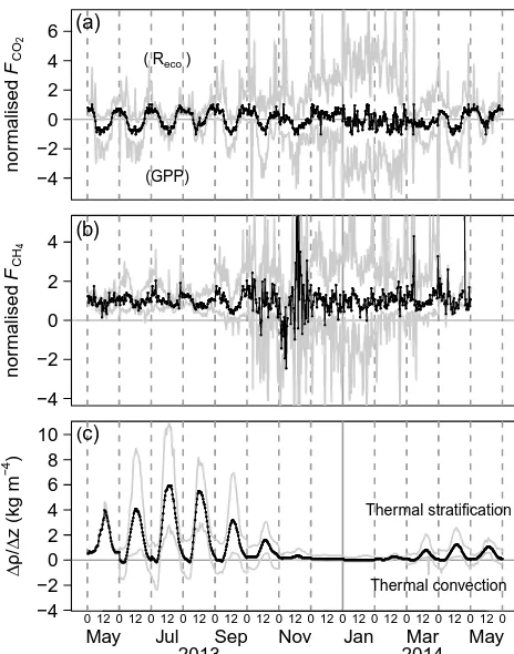
minimum/maximum and median of the half-hourly fluxes of the specific month (modified from Rinne et al., 2007). A pro-nounced diurnal cycle of CO2fluxes with peak uptake around
● ●●●●● ● ● ●● ● ● ● ●●● ● ● ● ●●●●●● ● ●●●●●●●●●● ● ●●●●●●●●●●● ● ● ● ●●●●● ● ● ● ● ● ● ● ● ●● ● ●●●●● ● ●●●●●●●●●●●● ● ● ●●● ● ● ● ● ● ● ● ● ●●●● ● ●●● ● ●● ●● ● ● ● ●●●● ●●● ●●●● ●●●●● ●● ●●●●●● ● ● ● ● ● ●●●●●●●●●● ● ●●●● ● ●● ● ● ● ● ● ●●● ● ●●●●●●● ●● ●●●●●●● ●●● ● ● ● ● ● ● ● ● ● ● ●●●●● ● ● ●● ●●●●●●●●●●●●●●●● ●●●● ● ● ● ●● ● ● ●●●●● ●● ● ● ●● ● ●●●● ● ● ● ● ● ●●●●● ● ●●●●● ● ● ● ● ●●●● ● ●●●●● ● ● ● ● ●●● ● ●● ● ●● ● ● ●● ●● ● ●● ● ● ●●● ● ● ● ● ●●●● ● ● ● ● ● ● ● ● ● ●●● ●●● ● ● ● ●● ● ● ● ● ● ●●●●● ●● ● ● ● ● ● ● ● ● ● ●●● ● ●● ● ●●● ● ● ● ●● ● ●● ●● ●●● ● ● ● ● ● ● ● ● ●● ● ● ● ●● ●● ● ● ● ● ● ●● ● ● ● ● ● ●● ●● ● ● ●● ● ● ● ● ● ● ● ●● ● ● ● ● ● ● ● ●●● ●● ● ● ● ● ● ● ● ● ● ● ● ● ● ● ● ● ●● ● ● ● ● ● ● ● ● ● ● ● ● ● ● ● ● ● ● ● ● ● ● ●● ● ●●●●●● ● ● ● ● ● ● ● ●●●●● ●●● ● ●●● ● ● ●●●●●●●●●●●● ● ●●●●● ● ● ●●●●●● ● ●●●● ●●● ● ● ● ● ●● ●●● ●●●●●●● ● ● ● ● ●● ●● ● ● ● ●●● ● ● ● ●●●●●● ● ●●●● ●● ● ●● ●●● ● ● ●● ● ● ● ● ● ● ● ● ● ● ● ●●●●●●●●●● ● ●●●● −4 −2 0 2 4 6 nor malised FC O2 ● ●●●●● ● ● ●● ● ● ● ●●● ● ● ● ●●●●●● ● ●●●●●●●●●● ● ●●●●●●●●●●● ● ● ● ●●●●● ● ● ● ● ● ● ● ● ●● ● ●●●●● ● ●●●●●●●●●●●● ● ● ●●● ● ● ● ● ● ● ● ● ●●●● ● ●●● ● ●● ●● ● ● ● ●●●● ●●● ●●●● ●●●●● ●● ●●●●●● ● ● ● ● ● ●●●●●●●●●● ● ●●●● ● ●● ● ● ● ● ● ●●● ● ●●●●●●● ●● ●●●●●●● ●●● ● ● ● ● ● ● ● ● ● ● ●●●●● ● ● ●● ●●●●●●●●●●●●●●●● ●●●● ● ● ● ●● ● ● ●●●●● ●● ● ● ●● ● ●●●● ● ● ● ● ● ●●●●● ● ●●●●● ● ● ● ● ●●●● ● ●●●●● ● ● ● ● ●●● ● ●● ● ●● ● ● ●● ●● ● ●● ● ● ●●● ● ● ● ● ●●●● ● ● ● ● ● ● ● ● ● ●●● ●●● ● ● ● ●● ● ● ● ● ● ●●●●● ●● ● ● ● ● ● ● ● ● ● ●●● ● ●● ● ●●● ● ● ● ●● ● ●● ●● ●●● ● ● ● ● ● ● ● ● ●● ● ● ● ●● ●● ● ● ● ● ● ●● ● ● ● ● ● ●● ●● ● ● ●● ● ● ● ● ● ● ● ●● ● ● ● ● ● ● ● ●●● ●● ● ● ● ● ● ● ● ● ● ● ● ● ● ● ● ● ●● ● ● ● ● ● ● ● ● ● ● ● ● ● ● ● ● ● ● ● ● ● ● ●● ● ●●●●●● ● ● ● ● ● ● ● ●●●●● ●●● ● ●●● ● ● ●●●●●●●●●●●● ● ●●●●● ● ● ●●●●●● ● ●●●● ●●● ● ● ● ● ●● ●●● ●●●●●●● ● ● ● ● ●● ●● ● ● ● ●●● ● ● ● ●●●●●● ● ●●●● ●● ● ●● ●●● ● ● ●● ● ● ● ● ● ● ● ● ● ● ● ●●●●●●●●●● ● ●●●● (a)
(Reco)
(GPP) ● ● ● ● ●● ●● ● ● ● ● ● ●●●●● ● ● ● ● ● ● ● ● ● ● ● ● ● ● ● ●●●●●● ● ● ● ● ● ●●●● ● ●● ●● ● ● ● ● ● ●●●●●● ● ● ● ● ● ●● ● ● ●●● ● ● ● ● ●●●●●● ● ●●● ● ●●●● ● ● ● ● ● ●● ● ● ● ●● ●●●● ● ●● ●●●●● ● ● ●● ● ● ● ● ●●●●●●● ● ● ● ● ● ● ● ● ● ●●●●●●●●● ●●● ● ● ● ● ●● ●● ● ● ● ●●●● ● ● ●●●●●●●●● ●●●●●●●●●●● ● ● ● ●●●● ● ● ● ● ● ●● ●● ● ● ● ● ● ● ● ● ● ● ● ● ●●●● ●●●●● ● ● ● ● ● ● ● ● ● ● ● ●● ● ● ● ● ● ● ● ● ● ● ● ● ● ● ● ● ● ● ● ● ● ● ● ● ● ●● ● ● ● ● ● ●● ● ● ● ● ● ● ● ● ● ●● ● ● ● ● ● ● ● ● ● ● ● ● ● ● ● ● ● ● ● ● ● ● ● ● ● ● ● ● ● ● ● ● ● ● ● ●● ● ● ● ● ● ● ● ● ● ● ● ● ● ● ● ● ●●● ● ● ● ● ● ● ● ● ● ● ● ● ● ● ● ● ● ●● ● ● ● ● ● ● ● ● ● ● ● ● ● ● ●● ● ● ● ●● ● ● ●● ● ● ● ● ● ● ● ● ● ● ● ● ●●● ● ● ● ●● ● ● ● ● ● ●●● ● ● ● ● ● ● ●●●● ● ● ● ● ● ● ● ●●● ●● ● ● ● ● ● ● ● ● ● ● ● ●●● ● ● ●●● ● ● ● ●● ● ●● ●● ● ● ● ● ● ● ● ● ● ● ● ● ● ● ●●● ● ●● ● ● ● ● ● ● ● ● ● ● ● ● ● ● ●●●●●●●●● ●●● ● ● ● ● ● ● ● ● ● ● ●● ● ● ● ● ● ● ● ● ● ● ● ● ● ● ● ● ● ● ● ● ● ●● ● ● ● ● ● ● ● ●● ● ● ● ●● ● ● ● ● ● ● ● ● ●● ● ● ● −4 −2 0 2 4 nor malised FC H4 ● ● ● ● ●● ●● ● ● ● ● ● ●●●●● ● ● ● ● ● ● ● ● ● ● ● ● ● ● ● ●●●●●● ● ● ● ● ● ●●●● ● ●● ●● ● ● ● ● ● ●●●●●● ● ● ● ● ● ●● ● ● ●●● ● ● ● ● ●●●●●● ● ●●● ● ●●●● ● ● ● ● ● ●● ● ● ● ●● ●●●● ● ●● ●●●●● ● ● ●● ● ● ● ● ●●●●●●● ● ● ● ● ● ● ● ● ● ●●●●●●●●● ●●● ● ● ● ● ●● ●● ● ● ● ●●●● ● ● ●●●●●●●●● ●●●●●●●●●●● ● ● ● ●●●● ● ● ● ● ● ●● ●● ● ● ● ● ● ● ● ● ● ● ● ● ●●●● ●●●●● ● ● ● ● ● ● ● ● ● ● ● ●● ● ● ● ● ● ● ● ● ● ● ● ● ● ● ● ● ● ● ● ● ● ● ● ● ● ●● ● ● ● ● ● ●● ● ● ● ● ● ● ● ● ● ●● ● ● ● ● ● ● ● ● ● ● ● ● ● ● ● ● ● ● ● ● ● ● ● ● ● ● ● ● ● ● ● ● ● ● ● ●● ● ● ● ● ● ● ● ● ● ● ● ● ● ● ● ● ●●● ● ● ● ● ● ● ● ● ● ● ● ● ● ● ● ● ● ●● ● ● ● ● ● ● ● ● ● ● ● ● ● ● ●● ● ● ● ●● ● ● ●● ● ● ● ● ● ● ● ● ● ● ● ● ●●● ● ● ● ●● ● ● ● ● ● ●●● ● ● ● ● ● ● ●●●● ● ● ● ● ● ● ● ●●● ●● ● ● ● ● ● ● ● ● ● ● ● ●●● ● ● ●●● ● ● ● ●● ● ●● ●● ● ● ● ● ● ● ● ● ● ● ● ● ● ● ●●● ● ●● ● ● ● ● ● ● ● ● ● ● ● ● ● ● ●●●●●●●●● ●●● ● ● ● ● ● ● ● ● ● ● ●● ● ● ● ● ● ● ● ● ● ● ● ● ● ● ● ● ● ● ● ● ● ●● ● ● ● ● ● ● ● ●● ● ● ● ●● ● ● ● ● ● ● ● ● ●● ● ● ● (b) ● ●●●●●●●●●●●●●●● ● ●● ●●● ● ● ● ● ●● ● ● ● ● ● ● ● ● ● ●● ● ●●●●●●●● ● ●●●●●●●●●●● ● ● ● ● ●● ● ● ● ●●●●●●●●● ● ● ● ● ● ● ● ● ● ● ● ●● ●●●●●●● ●●●●●●●●● ● ● ● ● ● ● ● ● ● ●●●●●●●●●● ● ● ● ● ● ● ● ● ● ● ● ● ● ● ● ●● ●●●●●●●●●●●●● ● ● ● ● ● ● ● ● ● ● ●●●●●● ● ● ● ● ● ● ● ● ● ● ● ● ● ● ●● ●● ●● ● ●●●●●●●●●●●●●●●●●● ● ● ●● ●●●●●●● ● ● ●● ● ● ● ● ● ●● ●●●●●●●●●●●●●●●●●●●●●●●●●●● ●●●●●●●●●●●●● ● ●●●●●●●●●●●●●●●●●●●●●●●●●●●●●●●●●●●●●●●●●●●●●●●●●●●●●●●●●●●●●●●●●●●●●●●●●●●●●●●●●●●●●●●●●●●●●●●●●●●●●●●●●●●●●●●●●●●●●●●●●●●●●●●●●●●●●●●●●●●●●●●●●●●●●●●●●●●●●●●●●●●●●●●●●●●●●●●●●●●●●●●●●●●●●●●●●●●●●●●●●●●●●●●●●●●●●●●●●●●●●●●●●●●●●●●●●●●●●●●●●● ● ●●●●●●●●●●●●●●●●●●●●●●●●●●●●●●●●●●●●●●●●●●●●●●● ●● ●●●●●●●●●●●●●●●●●●●●●●●●●●●●●●●●●●●●●●●●●●●●● ●●●●●●●●●●●●● −4 −2 0 2 4 6 8 10 ( ∆ρ / ∆ z (kg m − 4 ) ● ●●●●●●●●●●●●●●● ● ●● ●●● ● ● ● ● ●● ● ● ● ● ● ● ● ● ● ●● ● ●●●●●●●● ● ●●●●●●●●●●● ● ● ● ● ●● ● ● ● ●●●●●●●●● ● ● ● ● ● ● ● ● ● ● ● ●● ●●●●●●● ●●●●●●●●● ● ● ● ● ● ● ● ● ● ●●●●●●●●●● ● ● ● ● ● ● ● ● ● ● ● ● ● ● ● ●● ●●●●●●●●●●●●● ● ● ● ● ● ● ● ● ● ● ●●●●●● ● ● ● ● ● ● ● ● ● ● ● ● ● ● ●● ●● ●● ● ●●●●●●●●●●●●●●●●●● ● ● ●● ●●●●●●● ● ● ●● ● ● ● ● ● ●● ●●●●●●●●●●●●●●●●●●●●●●●●●●● ●●●●●●●●●●●●● ● ●●●●●●●●●●●●●●●●●●●●●●●●●●●●●●●●●●●●●●●●●●●●●●●●●●●●●●●●●●●●●●●●●●●●●●●●●●●●●●●●●●●●●●●●●●●●●●●●●●●●●●●●●●●●●●●●●●●●●●●●●●●●●●●●●●●●●●●●●●●●●●●●●●●●●●●●●●●●●●●●●●●●●●●●●●●●●●●●●●●●●●●●●●●●●●●●●●●●●●●●●●●●●●●●●●●●●●●●●●●●●●●●●●●●●●●●●●●●●●●●●● ● ●●●●●●●●●●●●●●●●●●●●●●●●●●●●●●●●●●●●●●●●●●●●●●● ●● ●●●●●●●●●●●●●●●●●●●●●●●●●●●●●●●●●●●●●●●●●●●●● ●●●●●●●●●●●●●
May Jul Sep Nov Jan Mar May
0 12 0 12 0 12 0 12 0 12 0 12 0 12 0 12 0 12 0 12 0 12 0 12 0 12 0
2013 2014
Thermal stratification
Thermal convection
[image:7.612.52.284.65.360.2]c)
Figure 3.Average diurnal cycle of(a)CO2flux,(b)CH4flux and (c)the water density gradient per month. The numbers at thexaxis denote midnight (00:00) and midday (12:00) in UTC. Midnight is also illustrated with a dashed line. Black and grey lines represent the mean and the range respectively. The CO2and CH4fluxes are nor-malised with the monthly minimum/maximum and the median of the half-hourly fluxes respectively. Although the zero line is slightly shifted due to normalisation, positive CO2fluxes roughly indicate the dominance ofRecoagainst GPP, negative fluxes the dominance of GPP againstReco. The period of ice cover was excluded from the calculation of the temperature gradient. A density gradient equal to or below 0 indicates thermally induced convective mixing down to the bottom of the open water body of the shallow lake; positive gra-dients indicate thermal stratification.
diurnal cycle of CH4 fluxes from June to September 2013
and in March 2014 (April 2014 based on 3 days only and May 2014 not available as the sensor was dismantled) with daily peaks during night-time (around midnight until early morning). The water density gradient indicates thermally in-duced convective mixing of the whole water column at the same time of the day from May until October 2013 and from February to May 2014. In May 2014 the diurnal pattern of the water density gradient was less pronounced than in May 2013.
May Jul Sep Nov Jan Mar May
0 500 1000 1500 Cum. G W P100 (g C O2 −eq. m − 2 a − 1 )
GWP100CO2+CH4
GWP100CO2
GWP100CH4
+1659
+525 +1134
[image:7.612.311.544.68.225.2]2013 2014
Figure 4. Cumulative GWP100 budgets of CO2 (based on MDSCO2nofoot), CH4 (based on NLRCH4nofoot)and the sum of
both for the EC source area during the observation period.
3.2 Gap-filling performance and annual budgeting of CO2, CH4, C and GWP
The MDSCO2nofoot approach explained 74 % of the
vari-ance in NEE (see Table 2). Median NEE accounted for 1.9 g CO2m−2 d−1. The annual budget of gap-filled NEE
(MDSCO2nofoot)between 14 May 2013 and 14 May 2014 was
524.5±5.6 g CO2m−2(see Table 3), characterising the site
as strong CO2source with moderate rates ofRecoand GPP.
We found a surprising CO2release strength during summer
2013, where already at the end of June dailyRecooften
ex-ceeded GPP. The highest daily CO2 emission and uptake
rates of 24.8 and−27.9 g CO2m−2d−1were both revealed in
the beginning of July 2013 (see Fig. 2). July 2013 accounted for 23.2 and 25.8 % of the annualRecoand GPP respectively.
In addition, net CO2release outside the growing season
(def-inition of the growing season following Lund et al., 2010; until 19 November 2013 and starting 26 February 2014) was 203.7 with a median of 2.2 g CO2m−2d−1.
The environmental variable giving the best NLR model for CH4was soil temperature in 10 cm depth (Ts10):
FCH4=exp(−7.224+0.313·Ts10). (7)
The model described 79 % of the variance in CH4 flux
(see Table 2). Including additional environmental variables to the regression function did not increase the model per-formance significantly. Cumulative CH4 emissions were
40.5±0.2 g CH4m−2a−1(see Table 3). Median CH4
emis-sions were 41.9 mg m−2d−1, peaked at the end of July 2013
with 0.6415 g CH4m−2d−1and were at the minimum in
Jan-uary 2014 (see Fig. 2). The month with the highest proportion of annual CH4 emissions was August 2013 (27.3 %).
Non-growing season CH4fluxes only accounted for a small
pro-portion within the annual budget, about 0.8 g CH4m−2.
-Table 2.Gap-filling model performance was estimated according to Moffat et al. (2007) with several measures (nCO2=6193,nCH4=3386,
fluxes of best quality QC 0): the adjusted coefficient of determination Radj2 for phase correlation (significant in all cases, p value < 2.2×10⁻¹⁶), the absolute root mean square index (RMSEabs)and the mean absolute error (MAE) for the magnitude and distribution of individual errors, as well as the bias error (BE) for the bias of the annual sums.
Method R2adj RMSEabs MAE BE
(mg m−230 min−1) (mg m−230 min−1) (g m−2a−1)
MDSCO2nofoot 0.74 104.35 24.05 13.14
NLRCO2foot 0.66 119.10 27.51 −2.12
NLRCH4nofoot 0.79 1.36 0.83 −3.34
[image:8.612.137.460.124.203.2]NLRCH4foot 0.81 1.28 0.78 −2.54
Table 3.Annual balances of CO2and CH4derived by different methods for the whole EC source area, the area of interest (AOI) and the two surface types: MDS approach without footprint consideration (MDSCO2nofoot)and NLR approach without (NLRCH4nofoot)and with
(NLRCH4foot, NLRCO2foot)footprint consideration. Uncertainty was calculated as square root of the sum of squared random uncertainty
(measurement uncertainty) and gap-filling uncertainty.
Source area Flux Method
(g m−2a−1) CO2 CH4
MDSCO2nofoot NLRCO2foot NLRCH4nofoot NLRCH4foot
Whole EC NEE 524.5±5.6 531.4±13.0
source area GPP −2380.5±5.6 −2122.1±16.7 Reco 2863.6±5.6 2603.6±8.4
CH4 40.5±0.2 39.8±0.2
AOI NEE 843.5±13.0
GPP −3192.2±16.7
Reco 4035.7±8.4
CH4 21.8±0.2
Emergent NEE 750.3±13.0
vegetation GPP −4076.8±16.7
Reco 4827.2±8.4
CH4 13.2±0.2
Open water NEE 158.2±13.0
GPP −1021.5±16.7
Reco 1179.7±8.4
CH4 52.6±0.2
Eq m−2a−1for the EC source area (see Fig. 4). The propor-tion of CO2in the C and GWP budget was 82.5 % and 31.6 %
respectively. Components of the annual net C balance other than CO2and CH4fluxes, e.g. dissolved C, are not
consid-ered in this study. Our uncertainty estimates are within the range of similar studies (e.g. Shoemaker et al., 2015). 3.3 Source area composition and spatial heterogeneity
of CO2and CH4exchange
Footprint analysis revealed the peak contribution in an av-erage distance of 18 m from the tower and mainly from the open water area of the shallow lake (see Fig. 5). Open wa-ter covered on average 62.5 % of the EC source area. The two surface types showed different emission rates in terms
of higher CH4fluxes and lower NEE rates with increasing
water (see Fig. 6). Within the NLRCO2foot approach both
surface types were denoted as sources of CO2but with about
4-fold stronger rates of GPP,Recoand NEE for emergent
veg-etation compared to open water (see Fig. 7 and Table 3). The approach yielded a similar cumulative annual NEE for the whole EC source area, including both surface types as the MDSCO2nofoot approach, but lower component fluxes (GPP
andReco). As for CO2, we implementedi as weighting
fac-tors within the NLR model for CH4(NLRCH4foot)to get the
[image:8.612.108.486.273.519.2]fractional coverage Ωi
wind direction (°)
0 20
40
60
80
100
120
140
160 180 200 220 240 260 280
300 320
340
0 0.2 0.4 0.6 0.8 1.0 0
20
40
60
80
100
120
140
160 180 200 220 240 260 280
300 320
340
0 0.2 0.4 0.6 0.8 1.0
[image:9.612.330.527.67.273.2]open water emergent vegetation
Figure 5.Source area fractioni of the two main surface types in dependence on the wind direction (2◦bins).
as follows:
FCH4=veg·exp(−10.076+0.415·Ts10)
+water·exp(−6.449+0.286·Ts10) . (8)
Open water accounted for more than 4-fold higher emis-sions than the vegetated areas (see Fig. 7 and Table 3). The NLRCH4foot approach revealed a similar annual CH4budget
as the NLRCH4nofootapproach.
Annual budgets of CO2 (844 g CO2m−2a−1) and CH4
(22 g CH4m−2a−1)for the AOI differed strongly from the
budgets for the EC source area due to the contrasting emis-sion rates of open water and emergent vegetation (see Ta-ble 3) and different fractional coverages of the surface types within the AOI and the EC source area. This resulted in a higher C loss (246.5 g C m−2a−1) and a lower GWP (1452.9 g CO2-Eq m−2a−1) for the AOI than for the EC
source area. In the following we will primarily discuss the budgets of the EC source area and the surface types.
4 Discussion
4.1 Diurnal variability of CH4emissions
In terms of its daily cycle, CH4 exchange between
wet-land ecosystems and the atmosphere is not generalisable but rather dependent on the spatial characteristics of the wetland and, thus, the impact of the individual CH4
emis-sion pathways (diffuemis-sion, ebullition, plant-mediated trans-port). Our measurements showed a diurnal cycle of CH4
ex-change from June to September 2013 and in March 2014, with the strongest emissions during night, as reported for shallow lakes (e.g. Podgrasjek et al., 2014) and wetland sites with a considerable fraction of open water (e.g. Godwin et
0.3 0.5 0.7 0.9
−15 −10 −5 0 5 10 15
−15 −10 −5 0 5 10 15 (
FC
O2
(µmol m
−
2 s
−
1 )
0.0 0.2 0.4 0.6 0.8 density
a)
0.3 0.5 0.7 0.9
0.0 0.1 0.2 0.3 0.4 0.5 0.6
fractional coverage Ωwater
FC
H4
(µmol m
−
2 s
−
1 )
0.0 0.5 1.0 1.5 2.0
[image:9.612.66.266.68.261.2](b)
Figure 6.Impact of the fractional coverage of open water (water) within the EC source area on the measured fluxes of CO2and CH4 (15 May to 14 September 2013). The abundances of CO2and CH4 fluxes in dependence onwaterare illustrated by a smoothed two-dimensional kernel density estimate. The variability of CO2 flux rates decreased with increasingwater, whereas the variability of the CH4flux increased.
al., 2013). In comparison, wetland CH4emissions were also
reported to show daily maxima at daytime (e.g. Morrisey et al., 1993; Hendriks et al., 2010; Hatala Matthes et al., 2014), especially at sites with high abundance of vascular plants. No diurnal pattern (e.g. Rinne et al., 2007; Forbrich et al., 2011; Herbst et al., 2011) occurred especially at sites without large open water areas (Godwin et al., 2013).
We assume the process of convective mixing of the water column (e.g. Godwin et al., 2013; Poindexter and Variano, 2013; Podgrajsek et al., 2014; Sahlée et al., 2014; Koebsch et al., 2015) to be crucial for the diurnal pattern of CH4
emis-sions at our study site. This is indicated by the concurrent timing of convective mixing and daily peak CH4emissions
and a generally high fractional source area coverage of the open water, which shows higher rates of CH4 release than
emergent vegetation. Furthermore, closed chamber measure-ments likewise show night-time peak emissions on the shal-low lake in summer 2013 (Hoffmann et al., 2015). During the day, CH4 is trapped in the lower (anoxic) layers of the
thermally stratified water column. Due to the heat release of the surface water to the atmosphere in the night the surface water cools down, initiating convective mixing of the wa-ter column down to the bottom. Diffusion is enhanced due to the buoyancy-induced turbulence, the associated increased gas transfer velocity at the air–water interface (Eugster et al., 2003; MacIntyre et al., 2010; Podgrajsek et al., 2014) as well as the transport of CH4enriched bottom water to the surface
May Jul Sep Nov Jan Mar May FC
H4
(g m
−
2 d
−
1 )
0 0.2 0.4 0.6 0.8
open water emergent vegetation (a)
May Jul Sep Nov Jan Mar May FC
O2
(g m
−
2 d
−
1 )
−30 −20 −10 0 10 20 30 40
GPP
Reco
NEE (b)
open water
May Jul Sep Nov Jan Mar May
FC O2
(g m
−
2 d
−
1 )
−30 −20 −10 0 10 20 30 40
2013 2014
GPP
Reco
NEE (c)
[image:10.612.69.266.68.391.2]emergent vegetation
Figure 7.Daily CH4, NEE and component fluxes (Recoand GPP) for the surface types:(a)daily CH4flux of open water and emer-gent vegetation;(b)daily NEE and component fluxes for open wa-ter;(c)daily NEE and component fluxes for emergent vegetation, derived by NLR with the source area fractions of the surface types (i)as weighting factors (NLRCH4foot, NLRCO2foot).
ebullition can be triggered by turbulence due to convective mixing (Podgrajsek et al., 2014; Read et al., 2012). Apart from convective mixing, highest sediment and soil tempera-ture in the night until early morning might play an important role for the peak emissions of CH4due to increased microbial
activity. Furthermore, diurnal variability in CH4 oxidation
could contribute to the daily pattern of CH4release. Oxygen
is supplied to the water, sediment and soil during the day in consequence of photosynthesis and increases CH4oxidation.
However, convective mixing of the water column during the night might supply oxygen to deeper water depths potentially increasing CH4oxidation. We assume plant-mediated
trans-port to be characterised by a reverse diurnal cycle with peak emissions during daytime, as the release of methane is depen-dent on the stomatal conductance of the plants (e.g. Morrisey et al., 1993). This pathway is limited to plants with aerenchy-matous tissue like Typha latifolia, which dominates the eu-littoral zone at our study site. CH4 is transported from the
soil to the atmosphere, bypassing potential oxidation zones
above the rhizosphere (chimney effect). Unusually for wet-land plants (Torn and Chapin, 1993), complete stomatal clo-sure during night was observed forTypha latifolia (Chan-ton et al., 1993). However, this temporal constraint seems to be superimposed by more efficient CH4pathways during the
night and early morning. Apart from CH4, thermally induced
convection potentially contributes also to the diurnal fluctu-ation of the CO2flux at our study site. According to Eugster
et al. (2003) penetrative convection might be the dominant mechanism yielding CO2fluxes during periods of low wind
speed, especially in case of a stratification of CO2
concen-trations in the water body. Ebullition triggered by convec-tive mixing might be less important for CO2than for CH4,
as concentrations of CO2are most often low in gas bubbles
(e.g. Casper et al., 2000; Poissant et al., 2007; Repo et al., 2007; Sepulveda-Jauregui et al., 2015; Spawn et al., 2015). Further investigations should focus on the controls of the di-urnal patterns in CO2and CH4exchange based on additional
measurements, e.g. gas concentrations in the water, methane oxidation or plant-mediated transport.
4.2 Annual CH4emissions
The CH4emissions of our studied ecosystem were within the
range of other temperate fen sites rewetted for several years (up to 63 g CH4m−2a−1; e.g. Hendriks et al., 2007; Wilson
et al., 2008; Günther et al., 2013; Schrier-Uijl et al., 2014). This rate is remarkably higher than the emission factor of 28.8 g CH4m−2a−1that was assigned to rewetted rich,
tem-perate organic soils, which is in turn more than twice the rate of the nutrient-poor complement (IPCC, 2014). In contrast, newly rewetted fens emit its multiple. In the first year after flooding, Hahn et al. (2015) observed at a fen site in NE Ger-many an average net release of 260 g CH4m−2a−1, which
is 186 times higher than before flooding. Two years later the CH4emissions were considerably lower (40 g CH4m−2
within the growing season; Koebsch et al., 2015). However, natural (e.g. Bubier et al., 1993; Nilsson et al., 2001) and de-graded fens (Hatala et al., 2012; Schrier-Uijl et al., 2014; see also IPCC, 2014) release most often less CH4than the
ma-jority of rewetted fens, with some exceptions (e.g. Huttunen et al., 2003).
The two main surface types open water and emer-gent vegetation differed substantially in their CH4
ex-change rates. Open water contributed overproportionally to the measured ecosystem fluxes and showed remark-ably higher CH4 release rates (52.6 g CH4m−2a−1) than
the emergent vegetation stands (13.2 g CH4m−2a−1).
How-ever, closed-chamber measurements at the shallow lake show an even higher long-term average annual CH4 release rate
(206 g CH4m−2a−1)since rewetting with large interannual
variability and occasionally extreme high release rates (up to 400 g CH4m−2a−1).
Table 4.NEE and net CH4exchange at open water sites. The letters in parentheses indicate seasonal (S; May to October) and annual (A) budgets. Positive water level indicates inundated conditions. GHG flux measurement methods are denoted as CH for chambers, CO for concentration profiles and TR for gas traps.
Reference Location, Dominant Study year Average NEE CH4
ecosystem type plant species water depth
(m) (g CO2m−2a−1) (g CH4m−2a−1)
Huttunen et al. (2003), CH Lake Postilampi, Finland: 1997 3.2 16 (A)
hypertrophic lake
Casper et al. (2000), TR/CO Priest Pot, UK: 1997 2.3 13 (A)
hypertrophic lake
Ducharme-Riel et al. (2015), CO Bran-de-Scie, Québec: 2007–2008 3.2 224 (A) eutrophic lake
Wang et al. (2006), CH Taihu Lake, China, 2003–2004
hypertrophic lake:
– bare infralittoral zone 0.5 to 1.8 3 (A)
– pelagic zone 1.8 4 (A)
Hendriks et al. (2007), CH Horstermeer, 2005 > 0 47 (A)
the Netherlands: 2006 > 0 49 (A)
eutrophic ditches
Waddington and Day (2007), CH Bois-des-Bel peatland, 2000–2002 Québec:
– ponds > 0 0.3 (S)
– ditches > 0 2.9 (S)
Naimann et al. (1991), CH Kabetogama Peninsula, Utriculariaspp., 1988
Minnesota, beaver pond: Potamogetonspp. 14 (A)
– submergent aquatic plants 0.45 12 (A)
– deep water 1.25
Roulet et al. (1992), CH Low forest region, Ontario: 1990 0.2 to 0.4 7.6 (A)
beaver ponds
Bubier et al. (1993), CH Clay Belt, Ontario: 1991 0.5 to 1.5 44 (A)
beaver pond
Yavitt et al. (1992), CH New York, beaver ponds: 1990
– 3 years old ≤2 34 (A)
– > 30 years old ≤2 40 (A)
mud deposited at the bottom of the open water body (which is typical for shallow lakes in rewetted fens), to be of par-ticular importance for high CH4 emissions as substrate for
decomposition. The mud initially evolved as a mixture of sand and easily decomposable labile plant litter from reed ca-nary grass, which died off after flooding and produced a large C pool for CH4production (Hahn-Schöfl et al., 2011).
Dur-ing an incubation experiment with substrate from our study site, Hahn-Schöfl et al. (2011) observed that the new sed-iment layer has very high specific rates of anaerobic CH4
(and CO2)production. In addition, Zak et al. (2015)
empha-sised the impact of litter quality and reported a very high CH4production potential for litter ofCeratophyllum demer-sum, which dominates the biomass in the open water at our study site. Due to the eutrophic character of the lake and as-sociated high productivity within the open water body and in the eulittoral zone, high amounts of fresh labile organic matter continuously replenish the mud layer and thus the C pool. Especially in the case of strong winds we further as-sume a lateral input of allochthonous organic matter into the
NE “bay” of the shallow lake, which is the area with the peak contribution of our EC derived fluxes, and thus an additional refill of the C pool. The importance of fresh labile organic matter provided by the die-back of the former vegetation as driving force for high CH4 emissions was also discussed in
Hahn et al. (2015). They measured the highest CH4
emis-sions in sedge stands suffering from strongest die-back. For comparison annual budgets of CH4and CO2for other
nutrient-rich lentic freshwater ecosystems in terms of pris-tine, anthropogenically influenced and transient ecosystems are listed in Table 4. Studies on nutrient-rich lakes gener-ally revealed lower CH4release for open water. In contrast,
beaver ponds were partially reported to emit comparable rates of CH4. Similarly to our study site beaver ponds are
at least in the beginning disbalanced ecosystems due to a rapidly increased water level with associated suffering and fi-nally the die-back of former vegetation, which is not adapted to higher water levels. A large C pool for CH4production
30 years CH4emissions still accounted for 40 g CH4m−2a−1
(Yavitt et al., 1992).
The lower CH4 emissions of the surface type emergent
vegetation might be the result of increased CH4 oxidation
in the soil, as plants with aerenchymatous tissue release oxy-gen into the rhizosphere, in reverse to the emission of CH4
into the atmosphere (Bhullar et al., 2013). Minke et al. (2015) highlight the difference in net CH4release for typical
helo-phyte stands with moderate emissions forTyphadominated sites. Besides the effect of the gas transport within plants, lower water and sediment temperatures due to shading by the emergent vegetation might yield lower CH4production
than for open water. Furthermore, the soil of emergent veg-etation stands is generally only temporarily and partly inun-dated and the water table decreased additionally during the unusual warm and dry summer 2013, probably resulting in a lower rate of anaerobic decomposition to CH4and a higher
rate of CH4 oxidation in the aerated top soil. This in turn
might be a reason that in comparison to other sites domi-nated byTypha(rewetted wetlands, lake shores and freshwa-ter marshes; see Table 4) the emergent vegetation at our site is at the lower limit of reported CH4release rates and best
comparable to closed chamber measurements ofTypha
lati-foliamicrosites at another rewetted fen site in NE Germany
(Günther et al., 2015).
4.3 Annual net CO2release
We observed high annual net release of CO2 during the
observation period, which is rather uncommon for fens several years after rewetting (e.g. Hendriks et al., 2007; Schrier-Uijl et al., 2014; Knox et al., 2015). Surprisingly, the net CO2 budget was higher or similar to those of
some drained and degraded peatlands (e.g. Hatala et al., 2012; Schrier-Uijl et al.; 2014, but IPCC, 2014). Both sur-face types acted as net sources, with emergent vegetation (750 g CO2m−2a−1) showing a distinctively higher net
bud-get (158 g CO2m−2a−1)as well as GPP andRecorates than
open water. Only a few NEE rates are published for the open water body of eutrophic shallow lakes. Ducharme-Riel et al. (2015) report 224 g CO2m−2a−1as annual NEE of a
eu-trophic lake in Canada (see Table 4). According to Korte-lainen et al. (2006), Finnish lakes, which are mainly small and shallow, continuously emit CO2 during the ice-free
pe-riod, positively correlated with their trophic state.
Our study revealed a high annual net CO2release for
emer-gent vegetation, which is in the wide range of NEE rates for
Typhasites reported in other studies, including both net CO2
sources and sinks (see Table 5). GPP and Reco are
gener-ally high (especigener-ally at rewetted fen sites; both component fluxes most often > 3000 g CO2m−2a−1), characterising Ty-phastands as high turnover sites, usually resulting in net CO2
uptake. In contrast,Recoand GPP rates at our study site are in
the lower part of the reported range. We assume the continu-ously highRecorates during winter 2013/2014, contributing
to the high annual net CO2emissions, to be the result of mild
and dry meteorological conditions. In summer 2013,Reco
ex-ceeded GPP already in late June, indicating a significant con-tribution of heterotrophic respiration to the CO2production.
Unusual warm and dry conditions and associated water table lowering during summer 2013 might have triggered a shift from anaerobic to aerobic decomposition due to the exposure of formerly only shallowly inundated soil and organic mud, primarily in the emergent vegetation stands. We could not observe a considerable decrease of the spatial extent of the open water body as emergent vegetation mainly covers the shallower edges of the water body. The effect of water table lowering atTyphasites due to dry conditions is also shown by Günther et al. (2015) and Chu et al. (2015): relative increase ofRecorates, resulting in net CO2release. This might be of
special interest in terms of climate change, as a temperature increase and significantly less precipitation in summer are expected for NE Germany and meteorological conditions are more frequently characterised as “unusually” warm and dry. In addition, a considerable increase of microbial activity and, thus, generally increased decomposition due to high temper-atures might be of importance. Besides CH4, Hahn-Schöfl
et al. (2011) showed that the new sediment layer at the bot-tom of inundated areas exhibits very high rates of anaerobic CO2 production. Allochthonous organic matter import into
the NE bay due to lateral transport, as discussed for CH4,
might have further enhanced decomposition (e.g. Chu et al., 2015). Longer data gaps in summer 2013 (see Fig. A1 in Ap-pendix A) increase the uncertainty of our annual CO2budget.
However, the observed shift to net CO2release starting in late
June 2013 as well as its continuation later on are substantially based on measurements.
4.4 Global warming potential and the impact of spatial heterogeneity
The lake ecosystem is characterised by a strong climate im-pact 9 years after rewetting, mainly driven by high CH4
emis-sions. Based on our results the site can hardly be classi-fied into any rewetting phase of the concept discussed by Augustin and Joosten (2007). Our results imply a delayed shift of the ecosystem towards a C sink with reduced cli-mate impact, which might be the result of the exceptional characteristics represented by eutrophic conditions and lat-eral transport of organic matter within the open water body. The trophic status of water and sediment is an important fac-tor regulating GHG emissions, as shown by Schrier-Uijl et al. (2011) for lakes and drainage ditches in wetlands. How-ever, the unusual meteorological conditions during our study period might have caused a differing (lower or higher) GWP compared to previous years. CH4emissions might have been
lower at the expense of high net CO2release, whereas under
usual meteorological conditions CO2 uptake, for example,
could probably compensate the CH4emissions. Inundation
dur-Table 5.Annual (A)/seasonal (S) NEE, GPP,Recoand net CH4exchange atTyphasites. Positive water level indicates inundated soil. GHG flux measurement methods are denoted as CH for chambers and EC for eddy covariance.
Reference Location, ecosystem type Dominant plant species
Study year Mean water level (m) NEE GPP (g CO2m−2a−1)
Reco CH4
(g CH4m−2a−1)
Kankaala et al. (2004), CH Lake Vesijärvi, Finland: – inner cattail–reed zone – outer cattail–reed zone
Phragmites australis, Typha latifolia Phragmites australis, Typha latifolia
1997 1998 1997 1998 1999
< 0.1 to > 0.2 < 0.1 to > 0.2 < 0.1 to > 0.2 < 0.1 to > 0.2 < 0.1 to > 0.2
51 (S)1 43 (S)1, 6 (S)2 30 (S)1
23 (S)1, 7 (S)2
23 (S)1
Chu et al. (2015), EC Lake Erie, Freshwater marsh
Typha angustifolia, Nymphaea odorata
2011 2012 2013
0.3 to 0.6 0.3 to 0.6 0.3 to 0.6
−289 (A) 109 (A) 340 (A)
−3338 (A) −3490 (A) −2666 (A)
3049 (A) 3599 (A) 3006 (A)
58 (A) 76 (A) 70 (A)
Bonneville et al. (2008), EC Strachan et al. (2015), NEE: EC, CH4: CH
Mer Bleue, Canada, freshwater marsh
Typha angustifolia 2005–2006 2005–2009
winter > summer ≈0
−967 (A) −462 to −1041 (A)
−3045 (A) 2078 (A) 170 (A)
Whiting and Chanton (2001), CH
Virginia, freshwater marsh
Florida, lake shore
Typha latifolia Typha latifolia
1992–1993 1992 1993
0.05 to 0.2 0.05 to 0.2 0.05 to 0.2
−3288 (A) −3587 (A) −4177 (A)
109 (A) 69 (A) 96 (A)
Rocha and Goulden (2008), EC San Joaquin Freshwater Marsh Reserve, Califor-nia:
– freshwater marsh
Typha latifolia 1999 2000 2001
winter+, midsummer – winter+, midsummer – winter+, midsummer –
−929 (A) 1887 (A)
−3994 (A) −6006 (A)
4811 (A)
5980 (A)
Knox et al. (2015), EC – wetland (rewetted 2010) – wetland (rewetted 1997)
Schoenoplectus acu-tus, Typhaspp. Schoenoplectus acu-tus, Typhaspp.
2012 2012
1.07 0.26
−1349 (A) −1455 (A)
−7717 (A) −5519 (A)
6721 (A) 4064 (A)
71 (A) 52 (A)
Petrescu et al. (2015), EC – wetland (rewetted 2010)
Typha latifolia 2010 0.51 388 (A) 21 (A)
Minke et al. (2015), CH Giel’ˇcyka˘u Kašyl, Belarus, fen (rewetted 1985)
Typha latifolia, Hydrocharis morsus-ranae
2010–2011 2011–2012
0.13 < 0.13
553 (A) −414 (A)
−2825 (A) −3980 (A)
3375 (A) 3566 (A)
80 (A) 91 (A)
Günther et al. (2015), CH Trebeltal, Germany, fen (rewetted 1997)
Typha latifolia 2011 2012
0.02 −0.09
−156 (A) 345 (A)
13 (A) 4 (A)
Wilson et al. (2007, 2008), CH Turraun, Ireland, cutover bog (rewetted 1991)
Typha latifolia 2002 2003
0.07 0.03
975 (A) 1653 (A)
−3272 (A) −4357 (A)
4064 (A) 6010 (A)
39 (A) 29 (A)
1Open water period;2winter.
ing rewetting the water table is generally recommended to be held at or just below the soil surface to prevent inundation and the formation of organic mud (Couwenberg et al., 2011; Joosten et al., 2012; Zak et al., 2015).
In contrast to CH4, the influence of water level on net
CO2release is not nearly consistent in the few existing
stud-ies of rewetted peatlands. In comparison to our site Knox et al. (2015) reported high net CO2uptake to substantially
com-pensate high CH4emissions for a site with mean water
lev-els above the soil surface after several years of rewetting (see Table 5). Similarly, Schrier-Uijl et al. (2014) reported high CO2 uptake rates for a Dutch fen site 7 years after
rewet-ting and even C uptake and a GHG sink function after 10 years with water levels below or at the soil surface. Herbst et al. (2011) present a snapshot of the GHG emissions of a Danish site after 5 years of rewetting with permanently and seasonally wet areas, whereby high CO2uptake and
moder-ate CH4emissions lead to substantial GHG savings. In
con-trast, weak CO2 uptake and decreasing, but still high, CH4
emissions were reported for another fen site in NE Germany with mean water levels above the soil surface (Koebsch et al., 2013, 2015; Hahn et al., 2015), resulting in a decreasing cli-mate impact after 3 years of rewetting. Interestingly, changes of NEE due to flooding were negligible, although GPP and Recorates decreased considerable due to the flooding
(Koeb-sch et al., 2013). In comparison to the decreasing CH4
emis-sions at this site, Waddington and Day (2007) report enhanc-ing CH4release for a Canadian peatland in the first 3 years
after rewetting. A third rewetted fen site in NE Germany with water levels close to the soil surface was reported as weak GHG source 14–15 years after rewetting (Günther et al., 2015).
We calculated the “true” fluxes of CO2 and CH4for the
[image:13.612.51.545.94.391.2]