The Pricing and Hedging of the Range Accrual Note

(1)

The Pricing and Hedging of the Range Accrual

Note

Gary Steven Licht

University of the Witwatersrand, Johannesburg

(2)

Abstract

The range accrual note is an exotic interest rate derivative that pays out a fixed rate for every day that a chosen reference rate falls within a predefined corridor. This project derives expressions for the price and ∆ of the range note before considering FRAs as a hedge instrument.

Acknowledgements

(3)

List of Figures

2.1 When the valuation date falls in the middle of the period, the valuation is split into two parts. The deterministic known period and the stochastic broken period . . . 11 2.2 The bottom time-line illustrates the case where the evaluation

date lies before the initiation of the first period while the time-line above it illustrates the case where the evaluation date falls in the middle of a period . . . 12 2.3 The top left graph gives the payoff for an in the money range

note paying out under low volatility. The bottom right graph is a spread of out of the money range notes (graphed above and next to it) paying out under high volatility . . . 14

3.1 Black’s model assumes that the underlying is marginally dis-tributed according to geometric Brownian motion at discrete points in time but makes no comment about the process be-tween these dates . . . 17 3.2 Timeline illustrating the procedure for finding the payoff as

a function of the numeraire . . . 18 3.3 This table illustrates how negligible the error term is in the

approximation forCPE. . . 21 3.4 Value surface of a 5-period range note as a function of time

and constant forward rate for a flat yield curve with initiation time 0.2, period 0.25, flat vol 0.1, upper strike 0.085, lower strike 0.07, nominal 100, fixed rate 0.08 and Days2 . . . 27

(6)

Chapter 1

Introduction

At initiation of the contract a range and rate are fixed, the range note pays the fixed rate for every day that the reference interest rate is in the corridor and nothing when it is not. The contract makes payments at periods equal to the tenor of the reference rate. This introduces timing issues into the pricing that make the daily replication of the note slightly more advanced than a simple spread of digital caplets. Instead the range note is replicated by daily range contingent payoffs which, themselves, are a spread of daily

contingent payoffs. The contingent payoff differs from the digital caplet in that, instead of paying out 1, it pays out the present value of 1 at the actual date of payment. The range note is then fully replicated by summing over all these range contingent payoffs for all ’active’ days in the future. Hence the pricing of the range note depends entirely on finding an expression for the contingent payoff.

The next chapter sets up the theory of the pricing procedure sketched in the above paragraph. After making the above more exact, we begin by con-sidering the two cases of the single period range note- when the evaluation date is before the initiation of the period and when it falls during the period. We then go on to show how multi-period range notes are built from these two cases.

Having established that pricing the range note depends entirely on evaluat-ing the contevaluat-ingent payoff, the third chapter accomplishes this in the South African market. A Black’s model is assumed for JIBAR, a suitable numeraire is chosen and an integral expression for the contingent payoff is found. This expression cannot be solved analytically1 _{and is, instead, approximated} nu-merically by Taylor expanding the integrand and interchanging summation and integral. This approximation then allows us to implement the pricing of the range note in matlab.

1

(7)

The fourth chapter is concerned with finding ∆ of the range note. Again this depends entirely on finding ∆ of the contingent payoff. The integral ex-pression for the contingent payoff is differentiated using theLeibnitz integral rule resulting in a boundary and integral term. The integral term is then solved with exactly the same method as that in chapter three. The rest of the chapter then gives thematlabalgorithm for finding ∆.

(8)

Chapter 2

General Method For Pricing

a Range Note

In this section we build up a general method for pricing a range note by considering a sequence of simpler derivatives. We will begin by considering the following instruments:

•European digital call option

•European range digital call option

•European contingent payoff call option

•European range contingent payoff call option

Before we discuss their relevance to the pricing of

•Single period range note

•Multi-period range note

2.1 European Digital Call Option

Definition: Adigital call is an option that has unit payoff if the reference interest rate is above the strike interest rate at maturity and zero if it is below or equal to the strike rate at maturity.

Let T, R(T, α) and k denote the options’s maturity, reference interest rate at maturity and strike rate respectively, whereαis the tenor of the reference interest rate. Then the payoff at maturityT is given by

(9)

0 onR(T;α)_≤k.

Thus with a suitable choice of numeraireφand equivalent martingale mea-sureQ we can price the digital call by evaluating

DC(t;T, α, k) =φ(t)EQ

θ(R(T;α)₋k)

φ(T)

(2.2)

2.2 European Range Digital Call Option

Definition: Arange digital call is an option that has unit payoff if the ref-erence interest rate is within the range (kL, kU] at maturity and zero outside

this range at maturity. We callkL the lower strike andkU the upper strike.

Denoting the range digital call byRD, we can mathematically express the definition as

RD(T;T, α, kL, kU) = 1;kL< R(T;α)≤kU

0;otherwise

= [θ(R(T;α)₋kL)−θ(R(T;α)−kU)] (2.3)

This payoff can be replicated with the following portfolio

•Long a digital call at the lower strike

•Short a digital call at the upper strike

Thus, by the law of one price we have that the price of a range digital call at datet(t < T) is

RD(t;T, α, kL, kU) =DC(t;T, α, kL)−DC(t;T, α, kU) (2.4)

2.3 European Contingent Payoff Call Option

Definition: A contingent payoff call is an option that pays at maturity

T the present value of one at a later time T′ _{if the reference interest rate}

is greater than the strike rate and zero if it is below or equal to the strike rate.

Denoting the present value atT of one atT′ _{by the discount factor}_Z₍_{T, T}′₎

and the contingent payoff call by CP, the payoff can be expressed as

CP T;T, T′_{, α, k}₌_Z₍_{T, T}′₎_θ₍_R₍_T_;_α₎₋_k₎

(10)

CP t;T, T′_{, α, k} ₌_φ₍_t₎_EQ

Z(T, T′₎_θ₍_R₍_T_;_α₎₋_k₎

φ(T)

(2.5)

2.4 European Range Contingent Payoff Call

Op-tion

Definition: A range contingent payoff call is an option that has payoff

Z(T, T′_{) if the reference interest rate is within the range (}_k

L, kU] at

matu-rity and zero outside this range at matumatu-rity.

Denoting the range contingent payoff call byRCP, we can express the payoff at maturity as

RCP T;T, T′_{, α, k}

L, kU=Z(T, T′) [θ(R(T;α)−kL)−θ(R(T;α)−kU)](2.6)

Analogously to the case of the range digital call, the range contingent pay-off call is a spread of contingent paypay-off calls and can be priced with the expression

RCP t;T, T′_{, α, k}

L, kU

=CP t;T, T′_{, α, k}

L

−CP t;T, T′_{, α, k}

U

(2.7)

2.5 Range Accrual Note

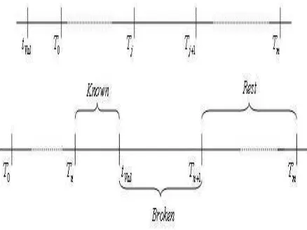
We begin the study of the range note by considering the basic single period range note, which has two cases. In the first case the valuation date falls before the initiation of the period and in the second case, the valuation date falls during the period. The second case is split into two parts: the deterministic period between the initiation of the period and the valuation date, and a truncated single period from the valuation date to the end of the period. This treatment of the single period range note then allows an easy description of the multiperiod range note.

2.5.1 Single Period Range Note

(11)

Valuation Date Before Period Initiation

Denoting the initiation and end of the period byT0 andT1 respectively, the fixed rate asRand the range note asV, the value of the range note atT1 is

V (T1;T0, T1, R, kL, kU) =

RN D

n X

i=0

[θ(R(T0+i;α)−kL)−θ(R(T0+i;α)−kU)]+N

(2.8) Where N is the nominal, D is the number of days in the year and T0+i is the ith day after T0 with T0 +n = T1. Obviously R(T0+i;α) is the reference interest rate on day T0 +i, which is known at T1, and so the summation counts the number of days in which the reference rate fell within the specified range over the period. Comparing this to (2.3) one might naively suspect that we can use digital calls as counters for the number of days and so replicate the range note with digital calls. However the payment of the digital call occurs at the same time as the reference rate is observed, thus ifkL < R(T0+i;α) ≤kU, the holder of the digital call would receive

one atT0+iwhereas a holder of the range note only receives this payment at T1. But if the holder received Z(T0+i, T1) at T0+i, then this payment would be worth one at T1 and we could replicate the range note. Thus we replicate the range note with the collection of range contingent payoffs

{RCP(t;T0+i, T1, α, kL, kU)}ni=0 giving

V (t;T0, T1, R, kL, kU) =

RN D

n X

i=0

RCP(t;T0+i, T1, α, kL, kU) +Z(t, T1)N (2.9) fort < T0.

Valuation Date During Period

(12)

[image:12.595.172.420.129.257.2]

Figure 2.1: When the valuation date falls in the middle of the period, the valuation is split into two parts. The deterministic known period and the stochasticbroken period

We call the period (T0, t] the known period as we have already observed how many days within this period will contribute to the payment at T1, we denote this number by H(t).

VKnown=

RN H(t)

D Z(t, T1)

Definingpsuch thatt=T0+p, we then price the contribution of thebroken

period (t, T1] in exactly the same way as in(2.9) except the summation now begins from i=p+ 1 as opposed to i= 0. Putting the parts together, we obtain

V (t;T0, T1, R, kL, kU) =

RN H(t)

D Z(t, T1)+ RN

D

n X i=p+1

RCP(t;T0+i, T1, α, kL, kU)+Z(t, T1)N (2.10)

forT0 < t≤T1.

2.5.2 Multi-Period Range Note

Definition:Amulti-period range note is a successive series of single period range notes with interest being paid at the end of each period and the nom-inal payment occurring at the end of the fnom-inal period.

We will only consider the case 1 where the fixed rate and strike range are constant throughout the life of the range note2_.

Define

1

The generalisation is obvious

2

(13)

Vj(t;Tj−1, Tj, R, kL, kU) =

RN D

nj

X i=0

RCP(t;Tj−1+i, Tj, α, kL, kU) (2.11)

Where Tj = Tj−1+nj. Then a m−period range note V, with initiation

date of first periodT0 and end dateTm of themth period, has value at date

t < T0 of

V (t;T0, Tm, R, kL, kU) = m X j=1

Vj(t;Tj−1, Tj, R, kL, kU) +Z(t, Tm)N (2.12)

[image:13.595.188.407.331.495.2]

WhereVj is given by (2.11),RCP by (2.7) and CP by (2.5).

Figure 2.2: The bottom time-line illustrates the case where the evaluation date lies before the initiation of the first period while the time-line above it illustrates the case where the evaluation date falls in the middle of a period

In the case where Tn < t≤ Tn+1 (n < m), we make the obvious adjust-ments to (2.12) and (2.10) to obtain

V (t;Tn, Tm, R, kL, kU) = Vn+1(t;Tn, Tn+1, R, kL, kU) +V (t;Tn+1, Tm, R, kL, kU) (2.13)

Vn+1(t;Tn, Tn+1, R, kL, kU) =

RN H(t)

D Z(t, T1) + RN

D

nn+1 X i=p+1

RCP(t;Tn+i, Tn+1, α, kL, kU)

(14)

2.5.3 The Utility of The Range Note

To tease out the financial understanding of a range note we begin by com-paring it to the most common of pure interest rate derivatives- the bond. A bond has a fixed coupon with fixed payment dates with a bullet accom-panying the last coupon payment. The future cash flows of the bond are completely deterministic and the interest rate dependence enters with the present valuing of these flows3. This is the basis for the inverse relationship between bonds and rates. The higher the rate, the lower the discount factor and the smaller the present value of the cash flow. The differing maturity of the bonds determines the exposure of the bond to the term structure of interest rates.

A range note also entitles the holder to cash flows at known dates including a known bullet at the end. However these cash flows are stochastic depend-ing on the daily level of some reference interest rate and are floored to be positive. This gives the holder of the range note direct exposure to the ref-erence rate and not just to an averaging of the yield curve as in the case of bonds. In addition, the details of the stochastic dependence of the payoff are a direct play on the reference interest rate volatility where the specification of the in the money corridor allows one to make this play as fine or coarse as desired. The purchaser of an in the money range note is expecting volatility to be low. An out of the money range note pays off for high volatility and a directional move up or down. While a spread of out of the money range notes pays off under high volatility regardless of the directional move. In addition the binary, all-or-nothing nature of the daily payoff makes this a relatively cheap derivative.

3

(15)

[image:15.595.131.465.130.411.2]

(16)

2.6 Pricing Schematic

Below is a summary for the pricing of a range note:

CP(t;T, T′_{, α, k}_{) =}_φ₍_t₎_EQhZ(T,T′₎_θ₍_R₍_T_;_α₎₋_k₎

φ(T)

i

RCP(t;T, T′_{, α, k}

L, kU) =CP(t;T, T′, α, kL)−CP (t;T, T′, α, kU)

Vj(t;Tj−1, Tj, R, kL, kU) = RND Pnj

i=0RCP(t;Tj−1+i, Tj, α, kL, kU)

Fort < T0

V (t;T0, Tm, R, kL, kU) =Pmj=1Vj(t;Tj−1, Tj, R, kL, kU) +Z(t, Tm)N

And for Tn< t≤Tn+1, we have

V (t;Tn, Tm, R, kL, kU) =Vn+1(t;Tn, Tn+1, R, kL, kU) +V (t;Tn+1, Tm, R, kL, kU)

Where

(17)

Chapter 3

Valuing a Range Note in the

South African Market

From this summary it is immediately evident that the valuation of a range note depends entirely on solving (2.5) for the contingent payoff call 1_{. In} this chapter we assume dynamics for forward JIBAR, choose a suitable nu-meraire, and evaluate (2.5).

3.1 Forward JIBAR Dynamics

We use Black’s model to price the contingent payoff by assuming that for-ward JIBARfi for periodti to ti+αhas marginal distribution on each day

given by solving the SDE

dfi =fiσidW (3.1)

Where dW is a brownian motion under the equivalent martingale measure and σi is the volatility measure.

We now solve forfi:

d(lnfi) =

1

fi

df₋ 1

2f2

i

(dfi)2

= ₋1 2σ

2

idt+σidW

Integrating fromtto later time tj (≤ti) gives

fi(tj) =fi(t) exp

−1₂σ2_i(tj−t) +σi p

tj −tz

; z_∼N(0,1) (3.2)

fi(t) are the forward JIBAR rates implied by the current yield curve 1

(18)

[image:18.595.169.424.128.253.2]

Figure 3.1: Black’s model assumes that the underlying is marginally distrib-uted according to geometric Brownian motion at discrete points in time but makes no comment about the process between these dates

Z(t, ti)

1 (1 +αfi(t))

=Z(t, ti+α)

⇒fi(t) =

1

α

Z(t, ti)

Z(t, ti+α)−

1

(3.3)

Now (3.2) holds for all pointstjwhere we assumefiis marginally distributed,

in our case this will just be at the payoff day ti. Hence (3.2) will give the

marginal distribution of j(ti;α) = fi(ti), the spot JIBAR rate from ti to

ti+α

j(ti;α) =fi(ti) =fi(t) exp

−1

2σ 2

i(ti−t) +σi√ti−tz

(3.4)

3.2 Evaluating a Contingent Payoff Call

We now evaluateCP(t;ti, T+α, α, k). We begin by rewriting the payoff in

(19)

[image:19.595.176.421.134.247.2]

Figure 3.2: Timeline illustrating the procedure for finding the payoff as a function of the numeraire

Givenj(ti;α) we know thatZ(ti, ti+α) = (1 +j(ti;α)α)−1. What does this

imply for Z(ti, T +α)?

Since α and τi are rational numbers, we know that there exists positive

integers m and n such that nτi = mα. Now if we invest n-times at the

τi-rate and m-times at the α-rate, then be no arbitrage we must have

Z(ti, T +α)n = Z(ti, ti+α)m ⇒Z(ti, T+α) = Z(ti, ti+α)

m n

⇒Z(ti, T+α) = Z(ti, ti+α)

τi α

⇒Z(ti, T+α) = (1 +j(ti;α)α)−

τi

α (3.5)

⇒Z(ti, T+α) =

1 +αfi(t) exp

−1₂σ_i2(∆ti) +σi p

∆tiz −τiα

(3.6)

We now choose the discount factorZ(t, ti+α) with fixed maturity atti+α

as the numeraire. Resultantly (2.5) becomes

CP(t;ti, T+α, α, k) = Z(t, ti+α)EQ

Z(ti, T +α)

Z(ti, ti+α)

θ(j(ti;α)−k)

= Z(t, ti+α)EQ h

(1 +j(ti;α)α)(1−

τi

α)θ(j(t

i;α)−k) i

= Z(t, ti+α)CPE(t;ti, T+α, α, k) (3.7)

Now the discount factor will be exogenously taken off the yield curve at t

and, so, the challenge becomes to solve for

CPE(t;ti, T +α, α, k) =EQ h

(1 +j(ti;α)α)(1−

τi

α)θ(j(t

i;α)−k) i

(20)

The strategy will be to Taylor expand (1 +j(ti;α)α)(1−

τi

α), interchange

in-tegral and summation before finding a series solution for the expectation. In order to implement this strategy, we require the following theorems.

3.2.1 Some Useful Theorems

Theorem (Binomial Series): For_|x_|<1 and0<_|β_|<1, we have

(1 +x)β =

∞

X n=0

(₋β)n

n! (−x)

n

where(₋β)nis the pochammer number defined in terms of the gamma func-tion as

(₋β)n=

Γ(n₋β) Γ(₋β)

Theorem(Weierstrass M-test): For eachn_≥0letfn:E →Rbe a continu-ous function. Suppose that for eachn_∈N_∃ Mn≥0such that|fn(x)| ≤Mn ∀x _∈E, and also PMn <∞, then Pfn(x) converges absolutely and uni-formly on E to some continuous function F

Theorem (Term-By-Term Integration): Suppose for each n _≥ 0 we have that fn : (a, b) → R is integrable over (a, b) and that Pfn converges uni-formly on (a,b) to some functionF : (a, b) _→R. ThenF is integrable over

(a, b) too and

Z b a

F(x)dx=

Z b a

∞

X n=0

fn(x) ! dx= ∞ X n=0 Z b a

fn(x)dx

3.2.2 Approximating CP_E

Settingβi= (1−τ i_α) we see that 0< βi <1 as long asτi 6= 0, α. Additionally,

in order to use the Binomial series we require

j(ti;α)α < 1 ⇒j(ti;α) <

1

α

⇒z < 1 σi√∆ti

−ln(fi(t)α) +1

2σ 2

i∆ti

=Du

Where we used (3.4) in the last line. Again using (3.4) we note that

θ(j(ti;α)−k) =θ(z−DL) (3.9)

where DL=

1

σi√∆ti

ln

k fi(t)

+1 2σ

2

i∆ti

(21)

As a quick check on the limits, we note that

DU =DL−

1

σi√∆ti

ln(kα) (3.11)

⇒ DL < DU ⇐⇒k <

1

α (3.12)

Using the Binomial series we can rewrite (3.8) as

CPE(t;ti, k) =

Z DU

DL

∞

X n=0

(₋βi)n √

2πn!

−αfi(t) exp

−1₂σ_i2(∆ti) +σi p

∆tiz n

exp

−1₂z2

dz

| {z }

I1

+

Z _∞ DU

(1 +j(ti;α)α)βiexp

−1₂z2

dz

√

2π

| {z }

Error Term

(3.13)

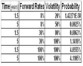
In order to approximate CPE by I1 we have to demonstrate that the error term is negligible. JIBAR is a quarterly rate implying thatα= 1₄. Thus the exclusion of the error term involves ignoring the expectation over the range

j(ti; 1/4) > 4. Both history and common sense would indicate that these

events truly are negligible. From an economic standpoint, before interest rates reach anywhere near 4 the mispricing of the derivative is the last of the writer’s problems. This is indeed evident in the mathematical framework of the model as shown in the table below whereP[z_≥DU] is calculated for

various choices of parameters. Even for long dated derivatives with current forward rate at 1 and high vol, we only have a 0.05 probability of the spot rate reaching 4. On the technical side this table also illustrates that the strike will, with almost certainty2 , also be below 4 showing by (3.11) that

DL≤DU.

2

(22)

[image:22.595.225.368.126.239.2]

Figure 3.3: This table illustrates how negligible the error term is in the approximation forCPE

Hence we will use the approximation

CPE(t;ti, k) ≈ Z DU

DL

∞

X n=0

(₋βi)n √

2πn!

−αfi(t) exp

−1₂σ_i2(∆ti) +σi p

∆tiz n

exp

−1₂z2

dz

= I1 (3.14)

In order to interchange integral and summation, we set

fn(z) = (−_nβ_!i)n −αfi(t) exp −1₂σ_i2(∆ti) +σi√∆tiznexp −1₂z2and, with

the aid of the Weierstrass M-test, check that the conditions set out in the theorem on term -by-term integration are satisfied:

•Γ(x) is an increasing function forx >2 implying that forn_≥3,

(−βi)n

n! =

Γ(n−βi)

Γ(−βi)n!

is a decreasing sequence in n since Γ(n−βi) < Γ(n) = (n−1)!

and Γ(₋βi) is finite for 0 < βi < 1. This together with fact that

(−βi)n

n!

is finite for all n implies that (−nβi!)n

≤γ∗ =max{ (−nβi!)n

|n= 0,1,2,3}.

Thus

P

|fn(z)|<Pγ∗ αfi(t) exp −1₂σ_i2(∆ti) +σi√∆tizn =Pγ∗νn<∞ on

z_∈(DL, DU) since ν <1 on this domain. Thus by the Weierstrass M-test

we can conclude that fn(z) is uniformly convergent on (DL, DU).

• Z DU

DL

|fn(z)|

dz

√

2π <

Z DU

DL

exp

−1₂z2

dz

√

2π <

Z ∞ −∞

exp

−1₂z2

dz

√

2π <∞

(23)

I1=

∞

X n=0

(₋βi)n

n!

−αfi(t) exp

−1₂σ_i2(∆ti)

nZ DU

DL

exp

−1₂z2+σi p

∆tiz

dz

√

2π

| {z }

I∗

(3.15) Solving for I∗ _gives

I∗ _{= exp}

1 2n

2_σ2

i∆ti Z DU

DL

exp

−1₂z₋nσi p

∆ti

2 _dz

√ 2π = exp 1 2n

2_σ2

i∆ti

Z DU−nσi

√

∆ti

DL−nσi√∆ti

exp −1 2z 2 dz √ 2π = exp 1 2n

2_σ2

i∆ti Z Dn

U

Dn L

exp

−1₂z2

dz √ 2π = exp 1 2n

2_σ2

i∆ti

[N(Dn_U)₋N(Dn_L)] (3.16) Where as usual N(x) denotes the cumulative normal function. Putting (3.16), (3.15) and (3.14) together, we have for 0< βi <1

CPE(t;ti, T +α, α, k) ≈

∞

X n=0

Γ(n₋βi)

Γ(₋βi)n!

−αfi(t) exp

−1₂σ_i2(∆ti(1−n)) n

[N(Dn_U)₋N(D_Ln)]

(3.17) Where

DL =

1

σi√∆ti ln k jt +1 2σ 2

i∆ti

DU = DL− 1

σi√∆ti

ln(kα)

Dn_L = DL−σi p

∆ti

D_Un = D_Ln₋ 1 σi√∆ti

ln(kα)

We now consider the case βi= 1. In this case we can solve (3.8) explicitly

•βi = 1⇐⇒τi= 0 :

CPE(t;T +α, T +α, α, k) =EQ[(1 +j(ti;α)α)θ(j(ti;α)−k)]

=

Z _∞ DL

1 +αfi(t) exp

−1₂σ2_i(T+α₋t) +σi√T +α−tz

exp

−1₂z2

dz

√

2π

= N(₋DL) +αfi(t) Z ∞

DL

exp

−1₂z₋σi √

T +α₋t2

dz

√

2π

= N(₋DL) +αfi(t)N(σi √

(24)

WhereDLis given by (3.10).

3.3 Matlab Implementation of Derived Scheme

In this section we implement the scheme set out in (2.15) with (3.8) as the expression for the contingent payoff. Note that the code assumes a flat volatility structure. If one were to generalise this, one would include a volatility curve in the body of the code and use it in an analogous fashion to the code for the term structure of forward rates taken off the discount curve.

3.3.1 The Discount Factor Function

Before we can implement the scheme proper we require a current discount curve in order to obtain

•the discounting of the expected payoff given by CPE.

•the current forward JIBAR rates which are inputs in CPE

The program implementing this will generally involve bootstrapping to ob-tain node points on a yield curve which will then be generated in full by some interpolation scheme. Since this is not a focus of the project, my gen-eration of discount factors is decidedly more sloppy. My function has two matrix inputs consisting of the node discount factors and their respective dates. Arbitrary discount factors are then obtained by linearly interpolating between these points. In the function below I have used node points3 as on Monday 3 October 2005:

function William=currentdiscount(T_start,T_maturity) df= [1.000000 0.999812... 0.342328]; T=[0...

0.002739726 13.26027397];

Znow1=interp1(T,df,T_maturity); Znow2=interp1(T,df,T_start); William=Znow1./Znow2;

3.3.2 Evaluating CP_E

%CPe for 0<beta<1

function Martin=CPe(alpha,tau,t,vol,f, strike,N) beta=1-tau./alpha;

Dlow=(log(strike./f)+0.5.*vol.^2.*t)./(vol.*sqrt(t)); Dup=(-log(f.*alpha)+0.5.*vol.^2.*t)./(vol.*sqrt(t)); b=0.5.*vol.^2.*t;

3

(25)

c=vol.*sqrt(t); a=alpha.*f; g=gamma(-beta); A=0;

for n=0:N

B=-b.*(1-n); C= n.*c;

A=A+ gamma(n-beta)./(g.*factorial(n))

.*(-a.*exp(B)).^n.*(cdf(Dup-C)-cdf(Dlow-C)); end

Martin=A;

%CpeEnd- Cpe for beta=1

function Malcolm=CPeEnd(alpha,t,vol,f, strike) Dlow=(log(strike./f)+0.5*vol^2*t)./(vol.*sqrt(t)); Malcolm=cdf(-Dlow)+alpha.*f.*cdf(vol.*sqrt(t)-Dlow);

3.3.3 Evaluating RCP_E

%RCPe for 0<beta<1

function Morris=RCPe(alpha,tau,t,vol,f, StrikeLow,StrikeUp,N)

Morris=CPe(alpha,tau,t,vol,f,StrikeLow,N)-CPe(alpha,tau,t,vol,f,StrikeUp,N);

%RCpeEnd- RCpe for beta=1

function Rachel=RCPeEnd(alpha,t,vol,f, StrikeLow,StrikeUp)

Rachel=CPeEnd(alpha,t,vol,f,StrikeLow)-CPeEnd(alpha,t,vol,f,StrikeUp);

3.3.4 Evaluating V_j

Denote Vj byV single.

function

Arthur=Vsingle(To,tvalue,alpha,vol,StrikeLow,StrikeUp,Nominal,rate,N)

t_i=[To+1/360:1/360:To+alpha-1/360]; Zend=t_i+alpha; tau=To+alpha-t_i; t=t_i-tvalue;

f=(DiscountFactor(t_i)./DiscountFactor(Zend)-1)./alpha;

fend=(DiscountFactor(To+alpha)./DiscountFactor(To+2.*alpha)-1)./alpha; Z=DiscountFactor(Zend);

RCP=RCPe(alpha,tau,t,vol,f,StrikeLow,StrikeUp,N); RN=Z.*RCP;

Arthur=(Nominal.*rate/360).*(sum(RN)+ DiscountFactor(To+alpha).*

(26)

3.3.5 Evaluating V _for t < T₀

function

Timothy=VBefore(m,To,tvalue,alpha,vol,StrikeLow,StrikeUp,Nominal,rate,N)

if tvalue>To

disp([’Error:tvalue>To. Use function V2Mid’]) else

PeriodValue=0; for j=0:m-1 T=To+j.*alpha;

PeriodValue=PeriodValue +

Vsingle(T,tvalue,alpha,vol,StrikeLow,StrikeUp,Nominal,rate,N); end

Timothy=PeriodValue+DiscountFactor(To+m.*alpha).*Nominal; end

3.3.6 Evaluating V _for T_n < t_≤T_n₊₁

We first calculate the value of the broken period

function

Allan=VBroken(To,tvalue,alpha,vol,StrikeLow,StrikeUp,Nominal,rate,N)

t_i=[tvalue+1/360:1/360:To+alpha-1/360]; Zend=t_i+alpha; tau=To+alpha-t_i; t=t_i-tvalue; Z=DiscountFactor(Zend); f=(DiscountFactor(t_i)./DiscountFactor(Zend)-1)./alpha;

fend=(DiscountFactor(To+alpha)./DiscountFactor(To+2.*alpha)-1)./alpha; RCP=RCPe(alpha,tau,t,vol,f,StrikeLow,StrikeUp,N); RN=Z.*RCP;

Allan=(Nominal.*rate/360).*(sum(RN)+DiscountFactor(To+alpha).*

RCPeEnd(alpha,To+alpha-tvalue,vol,fend,StrikeLow,StrikeUp));

Which is used in the calculation ofV mid

function

Walter=VMid(m,Days,To,tvalue,alpha,vol,StrikeLow,StrikeUp,Nominal,rate,N)

if tvalue<=To

disp([’Error: tvalue<=To. Use function V’]) else

Nodes=[To:alpha:To+(m-1)*alpha];

(27)

Broken=VBroken(NodeStart,tvalue,alpha,vol,StrikeLow,StrikeUp,Nominal,rate,N); Known=DiscountFactor(NodeStart+alpha).*Days.*rate.*Nominal/360;

Rest=VBefore(m-n-1,NodeStart+alpha,tvalue,alpha,vol

,StrikeLow,StrikeUp,Nominal,rate,N);

Walter=Broken+Known+Rest; end

3.4 Graphing a Value Surface: Flat Yield Curve

The underlyings of the range note are the MANY forward rates for the ref-erence rate on the remaining ’active’ days of the note. As such the pricing of the note in a market with any realistic structure is not amenable to graphical representation. Instead we use the current yield curve for the discounting and a flat yield curve to obtain the single forward rate. The value of the range note is then plotted against this forward rate and time to obtain a surface that illustrates the fundamentals of the pricing surprisingly well.

Thematlabcode for this involved some tampering with the previous code:

•CPe andRCPeremain unchanged

•The old DiscountFactoris renamed currentdiscount

•The functionDiscountFactornow has the flat yield as an extra argument and gives the corresponding discount curve

•VSingle,VBroken,VBeforeandVMidnow have this flat yield as an extra input

•The forward ratesf andf endappearing inVSingleandVBrokenare now obtained from the new function in DiscountFactor

(28)

0

0.5

1

1.5

0 0.05 0.1 0.15 0.2

90 92 94 96 98 100 102

Valuation Time Value Vs Constant Forward Rate & Valuation Time

Constant Forward Rate

[image:28.595.133.464.138.409.2]

Value

Figure 3.4: Value surface of a 5-period range note as a function of time and constant forward rate for a flat yield curve with initiation time 0.2, period 0.25, flat vol 0.1, upper strike 0.085, lower strike 0.07, nominal 100, fixed rate 0.08 and Days2

The first thing one notices is the jump at a day after the initiation date of the first period time = 0.201. This arises due to the fact that at this date we swap from usingV Bef ore toV M idwhich now has a deterministic input representing the number of in the money days we have observed in the current period. As such it is natural to distinguish between these two surfaces in the analysis.

(29)

The lines of constant time for both surfaces look like a normal density func-tion with mean near the middle of the in the money corridor flattening out very quickly at the limits of the corridor. The current forward value is the expected value of the spot at the ’pay day’ meaning the closer to this mean the forward rate is, the more area of its marginal distribution will fall in the money and vice versa for the tails at the edge of the corridor limits. This example is plotted with a low volatility and so the tails are quite thin, how-ever higher volatility inputs will result in fatter tails. The non-zero constant value the tails peteer off to is the present value of the bullet.

For lines of constant forward rate, we distinguish between the evolution of the flat base and that of the peaks. The base moves up quite linearly with time, this is just the fact that the present value of the bullet becomes greater having the net effect of adding a positive constant to the minimum value of the note to the time period before. This is true for both surfaces. Additionally, the peaks of these lines narrow as one moves forward in time. This is also true of both surfaces and occurs because the volatility of the forward rates decrease with time to maturity as in any theory with a geo-metric brownian motion assumption. Now the lines of constantf appearing on the peaks of both surface differ quite noticeably. They are increasing for

V Bef oreand decreasing forV M id. For the time period before the initiation of the first period, there are an equal number of days from which we might receive payment and the present value of these possible payments increase in time in such a way as they dominate the fluctuations in the ’possibility’ of these payments. However on theV M idsurface these lines decrease for two reasons. During the periods, they decrease because we have a constant input of 2 for Daysmeaning after the first two days there are no more observed in the money days. Between periods this peak will always drop as there are fewer possible payments left as compared to the period before.

(30)

Chapter 4

Delta of the Range Note

In this section we solve for ∆ in an analogous fashion to the numerical scheme set out for the pricing.

4.1 Evaluating Delta

The underlyings of the range note are the many forward ratesfi(T). Delta

is obtained by summing the partial derivatives of the range note with re-spect to each of these forward rates. Of course differentiating the numerical approximation for the value of the range note will not result in an accurate approximation for the first derivative. Instead we use the Leibnitz integral rule to differentiate the integral expression for the range note and then em-ploy the same procedure as in the previous section for approximating the integrals appearing in the expression for ∆ for the range note. The only dependence on fi(T) for the value of the range note is contained in the

in-tegralCPE.

(31)

∂

∂fiCP (t;T, T

′_{, α, k}_{) =}_Z₍_{t, t}

i+α)_∂f∂_iCPE(t;ti, T +α, α, k)

∆RCP(t;T, T′_{, α, k}

L, kU) = _∂f∂_iCP (t;T, T′, α, kL)−_∂f∂_iCP(t;T, T′, α, kU)

∆Vj(t;Tj−1, Tj, R, kL, kU) = RND Pnj

i=0∆RCP(t;Tj−1+i, Tj, α, kL, kU)

Fort < T0

∆V (t;T0, Tm, R, kL, kU) =Pmj=1∆Vj(t;Tj−1, Tj, R, kL, kU)

And for Tn< t≤Tn+1, we have

∆V (t;Tn, Tm, R, kL, kU) =Pmj=n+1∆Vj(t;Tj−1, Tj, R, kL, kU)

Where

∆Vn+1(t;Tn, Tn+1, R, kL, kU) = RN_D Pni=n+1p+1∆RCP(t;Tn+i, Tn+1, α, kL, kU) (4.1) Hence in order to solve for ∆ we need to approximate ∂CPE

∂fi .We begin by

stating the Leibnitz integral rule:

Theorem (Leibnitz Integral Rule): For a Riemann-integrable function f :

R2_→Rand differentiable functions a(y) and b(y), we have

∂ ∂y

Z b(y)

a(y)

f(y, z)dz=

Z b(y)

a(y)

∂f(y, z)

∂y dz+ ∂f

∂yf(y, a(y))− ∂f

∂yf(y, b(y))

Applying the Leibnitz integral rule to (3.8) gives

∂ ∂fi

CPE(t;ti, T+α, α, k) = EQ

∂ ∂fi

g(fi, z)θ(j(ti;α)−k)

−∂D_∂fL i

g(fi, DL) (4.2)

Where g(fi, z) = (1 +j(ti;α)α)(1−

τi

α) exp −

1 2z2

√

2π DL =

1

σi√∆ti

ln

k fi(t)

+ 1 2σ

2

(32)

4.1.1 Solving for the Boundary Term

We first do the easy bit and solve for the boundary term

∂DL

∂fi

= ₋ 1

fi(t)σi√∆ti

(4.3)

g(fi, DL) =

1 +fi(t)αexp

−1₂σ2_i∆ti+σi p

∆tiDL

(1−τiα) exp −1

2DL2 √

2π

= (1 +kα)1−ατ exp −

1 2D2L

√

2π

Where the last step follows from the fact that

expσi √

∆t= exp

(ln

k fi(t)

+ 1 2σ

2

i∆t

= k

fi(t)

exp

1 2σ

2

i∆t

Thus

∂g ∂fi

g(fi, DL) = 1

fi(t)σi√∆ti

(1 +kα)1−ατ exp −

1 2DL2

√

2π (4.4)

4.1.2 Solving for the Integral Term

We now begin the task of approximating the expectation in (4.2). Define

∆CPE =E

Q

∂ ∂fi

g(fi, z)θ(j(ti;α)−k)

(4.5)

Differentiating g gives

∂g ∂fi

=α1₋ τ

α 1 +fi(t)αexp

−1

2σ 2

i∆ti+σi p

∆tiz

−ατ exp

−12 z−σi

√

ti2 √

2π

Showing

∆CPE = (α−τ)

Z _∞ DL

1 +fi(t)αexp

−1₂σ2_i∆ti+σi p

∆tiz

−τ_α _exp ₋1 2z2

√

2π dz

≈ (α√−τ)

2π

Z Du

DL ∞ X n=0 τ α n n!

−fiαexp

−1₂σ2_i∆ti n

exp

σi p

∆tizn−

1 2

z₋σi p

∆ti 2

dz

= (α_√−τ) 2π

Z Du

DL ∞ X n=0 τ α n

n! (−fiα)

n_exp −1

2 z−σi

√

ti(n+ 1)2

(33)

Where the last line follows from grouping the exponentials and then com-pleting the square. The approximation follows from the truncation of the integral to Du as given in (3.11) in order for the binomial series to be

con-vergent over the integral. The justification for neglecting the rest of the domain is exactly the same as the discussion preceding figure 3.3. In or-der to interchange summation and integral we check that the conditions in the theorem on term-by-term integration are satisfied. To this end we set

hn(z) = (

τ

α)n

n! (−fiα)

n_exp

−12 z−σi

√

ti(n+ 1)2

and note

• Γ(x) is convex on (0,1) implying that Γ(τ /α) has a minimum, call it Γ∗_{. In addition Γ(}_x₎_≤_{1 on [1}_,_{2] and increasing on (2}_,_∞_{) showing that for}

n_≥1 we have Γ(n+τ /α) _≤Γ(n+ 1) =n! sinceτ /α <1. Thus for n_≥1, (τ /α)n

n! =

Γ(n+τ /α)

Γ(τ /α)n! ≤ Γ1∗. Also (τ /α)n

n! = 1 for n=1. Now setγ∗ =max{Γ1∗,1}, then _|hn(z)| ≤ γ∗(fiα)nexp −1₂(z−σi√∆ti(n+ 1)) ≤ ϕn < ∞ on z ∈

(DL, DU) since ϕ <1 on this domain. Thus by the Weierstrass M-test we

can conclude thathn(z) is uniformly convergent on (DL, DU).

• Z DU

DL

|hn(z)|

dz

√

2π < γ

∗

Z DU

DL

exp

−1₂z2

dz

√

2π < γ

∗

Z _∞

−∞

exp

−1₂z2

dz

√

2π <∞ (for fiα <1)

Hence

∆CPE ≈

(α₋τ)

√ 2π ∞ X n=0 τ α n

n! (−fiα)

nZ Du DL

exp

−1₂z₋σi p

∆ti(n+ 1) 2

dz

= (α√−τ)

2π ∞ X n=0 τ α n

n! (−fiα)

nZ Du−σi

√

∆ti(n+1)

DL−σi

√

∆ti(n+1)

exp

−1₂z2

dz

= (α₋τ)

∞ X n=0 τ α n

n! (−fiα)

nh_N₍_Dn′

U)−N(Dn

′

L) i

= (α₋τ)

∞

X n=0

Γ n+_ατ

Γ _ατn! (−fiα)

nh

N(Dn_U′)₋N(Dn_L′)i (4.7) Thus putting (4.4) and (4.7) together, we obtain forti 6=T +α

∂ ∂fi

CPE(t;ti, T +α, α, k) ≈ (α−τ)

∞

X n=0

Γ n+ τ_α

Γ _ατn! (−fiα)

nh_N₍_Dn′

U)−N(Dn

′

L) i

− 1

fi(t)σi√∆ti

(1 +kα)1−ατ exp −

1 2D2L

√

2π (4.8)

Where

D_Ln′ = DL−σi p

∆ti(n+ 1) =DnL−σi p

∆ti (4.9)

D_Un′ = DU−σi p

∆ti(n+ 1) =DnU−σi p

(34)

For the case whereτ = 0_⇔ti=T+α, we have an exact solution for CPE and differentiating (3.18) gives

∂ ∂fi

CPE(t;T +α, T +α, α, k) =

∂DL

∂fi

αfi(t)N′(σi √

T+α₋t₋DL) +N′(−DL)

+αN(σi √

T +α₋t)

= 1

fi(t)σi√∆ti

αfi(t)N′(σi √

T+α₋t₋DL) +N′(−DL)

= exp −

1 2D2L

fi(t)σi√2π∆ti

1 +αfi(t) exp

−1₂σ2_i(T+α₋t)₋σi √

T+α₋tDL

(4.11)

Where the first equality follows from (4.3) and the last equality follows from rewritingN′₍_σ

i√T +α−t−DL) in terms ofN′(−DL)

4.2 Matlab Implementation for Finding

∆

The above expression together with ∆-schematic (4.1) gives an algorithm for finding ∆ of the range note. This section contains the implementation of this scheme inmatlab.

4.2.1 Evaluating _∂f∂

i

CP_E

%DeltaCPe for 0<tau<1

function Meredith=DeltaCPe(alpha,tau,t,vol,f,strike,N) Dlow=(log(strike./f)+0.5.*vol.^2.*t)./(vol.*sqrt(t));

a=tau./alpha; b=vol.*sqrt(t); c=log(strike./alpha); D=Dlow-c./b; d=f.*alpha; g=gamma(a);

A=0; for n=0:N

A=A+gamma(n+a)./(g.*factorial(n)).*(-d).^n.*(cdf(D-b.*(n+1))-cdf(Dlow-b.*(n+1))); end

Meredith=(alpha-tau).*A

+(1./(f.*b.*sqrt(2*pi))).*(1+strike.*alpha).^(1-tau/alpha).*exp(-0.5.*Dlow.^2);

%DeltaCPe for tau=0

(35)

Margeret=exp(-0.5.*Dlow.^2)./(f.*q*sqrt(2*pi))

.*(1+alpha.*f.*exp(-0.5.*q.^2+q.*Dlow))+alpha.*cdf(q-Dlow);

4.2.2 Evaluating ∆RCP_E

%DeltaRCPe for 0<tau<1

function Kylie=DeltaRCPe(alpha,tau,t,vol,f,StrikeLow,StrikeUp,N) Kylie=DeltaCPe(alpha,tau,t,vol,f,StrikeLow,N)

-DeltaCPe(alpha,tau,t,vol,f,StrikeUp,N);

%DeltaRCPe for tau=0

function Ralph=DeltaRCPeEnd(alpha,t,vol,f, StrikeLow,StrikeUp)

Ralph=DeltaCPeEnd(alpha,t,vol,f,StrikeLow)-DeltaCPeEnd(alpha,t,vol,f,StrikeUp);

4.2.3 Evaluating ∆V_j

function

Rachel=Vsingle(To,tvalue,alpha,vol,StrikeLow,StrikeUp,Nominal,rate,N)

t_i=[To+1/360:1/360:To+alpha-1/360]; Zend=t_i+alpha; tau=To+alpha-t_i; t=t_i-tvalue;

f=(DiscountFactor(tvalue,t_i)./DiscountFactor(tvalue,Zend)-1)./alpha

fend=(DiscountFactor(tvalue,To+alpha)./DiscountFactor(tvalue,To+2.*alpha)-1)./alpha; Z=DiscountFactor(tvalue,Zend)

DeltaRCP=DeltaRCPe(alpha,tau,t,vol,f,StrikeLow,StrikeUp,N) DeltaRN=Z.*DeltaRCP

Rachel=

(Nominal.*rate/360).*(sum(DeltaRN)+DiscountFactor(tvalue,To+alpha)

.*DeltaRCPeEnd(alpha,To+alpha-tvalue,vol,fend,StrikeLow,StrikeUp));

4.2.4 Evaluating ∆V _for t_≤T₀

function

Tobias=DeltaVBefore(m,To,tvalue,alpha,vol,StrikeLow,StrikeUp,Nominal,rate,N)

if tvalue>To

disp([’Error:tvalue>To. Use function DeltaVMid’]) else

PeriodValue=0; for j=0:m-1 T=To+j.*alpha;

PeriodValue=PeriodValue

(36)

end end

Tobias=PeriodValue;

4.2.5 evaluating V _for T_n < t_≤T_n₊₁

We first calculate the value of the broken period

function

Howard=VBroken(To,tvalue,alpha,vol,StrikeLow,StrikeUp,Nominal,rate,N)

t_i=[tvalue+1/360:1/360:To+alpha-1/360]; Zend=t_i+alpha;

tau=To+alpha-t_i; t=t_i-tvalue; Z=DiscountFactor(tvalue,Zend);

f=(DiscountFactor(tvalue,t_i)./DiscountFactor(tvalue,Zend)-1)./alpha; fend=(DiscountFactor(To+alpha)./DiscountFactor(To+2.*alpha)-1)./alpha; DeltaRCP=DeltaRCPe(alpha,tau,t,vol,f,StrikeLow,StrikeUp,N);

DeltaRN=Z.*DeltaRCP;

Howard=(Nominal.*rate/360).*(sum(DeltaRN)+DiscountFactor(tvalue,To+alpha)

Which is used in the calculation of ∆V mid

function

Betty=DeltaVMid(m,Days,To,tvalue,alpha,vol,StrikeLow,StrikeUp,Nominal,rate,N)

if tvalue<=To

disp([’Error: tvalue<=To. Use function DeltaVBefore’]) else

NodeStart=max(Nodes.*(tvalue<=Nodes)); n=(NodeStart-To)./alpha;

DeltaBroken=DeltaVBroken(NodeStart,tvalue,alpha,vol,StrikeLow,StrikeUp,Nominal ,rate,N); DeltaRest=DeltaVBefore(m-n-1,NodeStart+alpha,tvalue,alpha,vol,StrikeLow,StrikeUp

,Nominal,rate,N);

(37)

4.3 Graphing

∆

: Flat Yield Curve

The Delta surface is obtained in the same manner as the value surface in

section 3.4 and its code is given in the same appendix A. In addition the function SolSurfSeperateplots line segments of the Delta and Value surfaces.

The matlab code for this involved some tampering with the code of the

previous section:

•DeltaCPe andDeltaRCPeremain unchanged

•The old DiscountFactoris renamed currentdiscount

•The functionDiscountFactornow has the flat yield as an extra argument and gives the corresponding discount curve

• DeltaVSingle, DeltaVBroken, DeltaVBeforeand DeltaVMid now have

this flat yield as an extra input

•The forward ratesfandf endappearing inDeltaVSingleandDeltaVBroken are now obtained from the new function inDiscountFactor

(38)

0

0.5

1

1.5

0 0.05 0.1 0.15 0.2 −800 −600 −400 −200 0 200 400 600 800 1000

Valuation Time Delta Vs Constant Forward Rate & Valuation Time

Delta

0 0.02 0.04 0.06 0.08 0.1 0.12 0.14 0.16 0.18 0.2 −600

−400 −200 0 200 400 600 800

DeltaVBefore

DeltaVBefore VS Constant Forward Rate

0 0.02 0.04 0.06 0.08 0.1 0.12 0.14 0.16 0.18 0.2 −800

−600 −400 −200 0 200 400 600 800 1000

DeltaVMid

DeltaVMid VS Constant Forward Rate

0 0.02 0.04 0.06 0.08 0.1 0.12 0.14 0.16 0.18 0.2 −300

−200 −100 0 100 200 300 400

DeltaVMid

[image:38.595.129.468.137.583.2]

DeltaVMid VS Constant Forward Rate

(39)

The lines of constant t are exactly as expected. These lines on the value surface look like a normal density function. Hence we would expect the ∆ of these lines to look like a derivative of the normal density function (up to some scaling factor given by the chain rule) which is exactly what we see. The additional structure can also be explained in relation to the value surface:

•The non-linear decreasing (increasing) lips of ∆V Bef orecan be explained by the fact that as we move forward in time the peak of the ’normal distrib-ution’ is increasing while the volatility is decreasing exaggerating the slopes on either side of the peak.

• The (symmetric) hills of the surface both narrow as time evolves. This is just a result of the fact that as we move forward in time, the ’normal distributions’ narrow causing the tails to flatten earlier.

(40)

Chapter 5

FRAs as a Hedge Instrument

for the Range Note

We begin this chapter by using FRAs to construct a hedge portfolio for the range note. We then derive an expression for the hedge slippage involved in this replication.

5.1 Creating the Hedge Portfolio

In this section we derive a hedge portfolio for the range note. As is explicit in the pricing, the range note can be decomposed into daily range contin-gent payoffs for all remaining ’pay days’. The forward rates beginning on each of these days over a periodα are the stochastic drivers of these deriv-atives. Hence it seems to natural to use FRAs as the hedge instrument. The total hedge portfolio will consist of a position in each of these FRAs and a position in a riskless money market account. That is each range con-tingent payoff RCP(t;ti, T +α, α, kL, kU) will be hedged with a position

in the FRA U(t;ti, ti +α) struck at Ri for the period ti to ti +α and a

position in the money market account M(t) = exp(r(t₋t0) wheret0 is the initiation date of the hedge andr is the risk free rate. To be ∆-hedged at every momenttwe require:

V(t) = RN

D

X i

RCP(t;ti, α, kL, kU) = X

i

φi(t)U(t;ti, ti+α) +µ(t)M(t)

(5.1)

∆V(t) = RN

D

X i

∆RCP(t;ti, α, kL, kU) = X

i

φi(t)

∂ ∂fi

U(t;ti, ti+α) (5.2)

(41)

money account respectively and are the variables we wish to solve for. We begin by findingU(t;ti, ti+α) and _∂f∂_iU(t;ti, ti+α).

The value of the FRA at timet is given by

U(t;ti, ti+α) = Z(t, ti)−Z(t, ti+α)

| {z }

floating leg

−RiαZ(t, ti+α)

| {z }

fixed leg

= Z(t, ti)−Z(t, ti)1 +Riα

1 +αfi

= Z(t, ti) 1 +αfi

[1 +αfi−1−Riα]

= αZ(t, ti)

1 +αfi

[fi−Ri] (5.3)

and so

∂ ∂fi

U(t;ti, ti+α) = −α2

Z(t, ti)

(1 +αfi)2

[fi−Ri] +α

Z(t, ti)

1 +αfi

= α Z(t, ti)

(1 +αfi)2

[1 +αfi−αfi+αRi]

= α Z(t, ti)

(1 +αfi)2

[1 +αRi] (5.4)

Putting (5.4) and (5.2) together and comparing term by term gives:

φi(t) =

RN D

∆RCP(t;ti, α, kL, kU) ∂

∂fiU(t;ti, ti+α)

= RN

D

(1 +αfi)2

αZ(t, ti)[1 +αRi]

∆RCP(t;ti, α, kL, kU) (5.5)

Which together with (5.1) gives

µ(t) = exp(₋r(t₋t0))

"

V (t;T0, Tm, R, kL, kU)− X

i

φi(t)U(ti, ti+α) #

(5.6) Thus the hedge portfolio Ω(t) is

Ω(t) =X

i

φi(t)U(t;ti, ti+α) +µ(t) exp(r(t−t0)) (5.7)

(42)

5.2 Cost of Refinancing

The first fundamental theorem of no arbitrage pricing says that a model is arbitrage free if and only if there exists an equivalent martingale measure. Hence with every martingale measure there exists a strategy that replicates the derivative. In particular the price of the derivative is the cost of replica-tion. This theory is developed in the world of continuous time and assumes that one continuously rebalances the hedge portfolio. In practice this is not possible and one can only rebalance the hedge in discrete time. This introduces a hedge slippage with an associated cost referred to as the cost of refinancing. This cost is the difference between the derivative and the hedge portfolio just before rebalancing. Let Π(jt+δt) denote the cost of refinancing associated with the periodjt to jt+δt then

Π(jt+δt) = V(jt+δt)₋

" X

i

φi(jt)U(jt+δt;ti, ti+α) +µ(jt) exp(r(jt+δt−t0))

#

= V(jt+δt)₋exp(r(jt+δt))V(jt)

−X i

φi(jt) [U(jt+δt;ti, ti+α)−exp(r(jt+δt))U(jt+δt;ti, ti+α)]

= δV(jt+δt)₋X

i

φi(jt)δU(jt+δt;ti, ti+α) (5.8)

Where the first equality is a definition and the second follows from (5.6). Now δV(jt +δt) is the difference between holding the derivative or sell-ing it and investsell-ing the cash in a bank account over δt and, similarly,

δU(jt+δt;ti, ti+α) is the difference between holding the FRA or selling it

and investing the cash in a bank account overδt. This makes sense as if the derivative and the underlying both grew at the risk free rate there would be no need to adjust the hedge. In fact we would just invest the original cost of the derivative in the bank.

The total cost of refinancing the range note Π(t, mt+δt) fromtto mt+δtis then obtained by summing over all of the readjustment points in this period

Π(t, mt+δt) =

m X j=1

(43)

Appendix A

Code for Sections 3.4 and 4.3

A.1 Discount Factors

function William=DiscountFactor(R,T_start,T_maturity) William=exp(-R.*(T_maturity-T_start));

%%%%%%%%%%%%%%%%%%%%%%%%%%%%%%%%%%%%%%%%%%%%%%%%%%%%%%%%%%%%%%%%%%%%%%%%%%%%

function earth=currentdiscount(T_start,T_maturity)

df= [1.000000 0.999812... 0.342328]; T=[0... 0.002739726 13.26027397];

Znow1=interp1(T,df,T_maturity); Znow2=interp1(T,df,T_start); earth=Znow1./Znow2;

A.2 Value Functions

function

Arthur=Vsingle(To,tvalue,alpha,vol,StrikeLow,StrikeUp,Nominal,rate,N,R)

t_i=[To+1/360:1/360:To+alpha-1/360]; Zend=t_i+alpha;

tau=To+alpha-t_i; t=t_i-tvalue;

f=(DiscountFactor(R,tvalue,t_i)./DiscountFactor(R,tvalue,Zend)-1)./alpha;

fend=(DiscountFactor(R,tvalue,To+alpha)./DiscountFactor(R,tvalue,To+2.*alpha)-1) ./alpha; Z=currentdiscount(tvalue,Zend);

(44)

Arthur=

(Nominal.*rate/360).*(sum(RN)+currentdiscount(tvalue,To+alpha)

.*RCPeEnd(alpha,To+alpha-tvalue,vol,fend, StrikeLow,StrikeUp));

%%%%%%%%%%%%%%%%%%%%%%%%%%%%%%%%%%%%%%%%%%%%%%%%%%%%%%%%%%%%%%%%%%%%%%%%%%%%%

function

Allan=VBroken(To,tvalue,alpha,vol,StrikeLow,StrikeUp,Nominal,rate,N,R)

Z=currentdiscount(tvalue,Zend);

fend=(DiscountFactor(R,tvalue,To+alpha)./DiscountFactor(R,tvalue,To+2.*alpha)-1) ./alpha; RCP=RCPe(alpha,tau,t,vol,f,StrikeLow,StrikeUp,N);

RN=Z.*RCP;

Allan=(Nominal.*rate/360).*(sum(RN)+currentdiscount(tvalue,To+alpha)

.*RCPeEnd(alpha,To+alpha-tvalue,vol,fend, StrikeLow,StrikeUp));

%%%%%%%%%%%%%%%%%%%%%%%%%%%%%%%%%%%%%%%%%%%%%%%%%%%%%%%%%%%%%%%%%%%%%%%%%%%%

function

Timothy=VBefore(m,To,tvalue,alpha,vol,StrikeLow,StrikeUp,Nominal,rate,N,R)

if tvalue>To

disp([’Error:tvalue>To. Use function V2Mid’]) else PeriodValue=0; for j=0:m-1 T=To+j.*alpha;

VSingle(T,tvalue,alpha,vol,StrikeLow,StrikeUp,Nominal,rate,N,R); PeriodValue=PeriodValue+Vsingle(T,tvalue,alpha,vol,StrikeLow,StrikeUp

,Nominal,rate,N,R); end

Timothy=PeriodValue+currentdiscount(tvalue,To+m.*alpha).*Nominal;

%%%%%%%%%%%%%%%%%%%%%%%%%%%%%%%%%%%%%%%%%%%%%%%%%%%%%%%%%%%%%%%%%%%%%%%%%

function

Walter=VMid(m,Days,To,tvalue,alpha,vol,StrikeLow,StrikeUp,Nominal,rate,N,R)

(45)

disp([’Error: tvalue<=To. Use function V’]) else

NodeStart=max(Nodes.*(tvalue>=Nodes)); n=(NodeStart-To)./alpha;

Broken=VBroken(NodeStart,tvalue,alpha,vol,StrikeLow,StrikeUp,Nominal ,rate,N,R); Known=currentdiscount(tvalue,NodeStart+alpha).*Days.*rate.*Nominal/360; Rest=VBefore(m-n-1,NodeStart+alpha,tvalue,alpha,vol,

StrikeLow,StrikeUp,Nominal,rate,N,R);

Walter=Broken+Known+Rest;

A.3 Delta Functions

function

Rachel=Vsingle(To,tvalue,alpha,vol,StrikeLow,StrikeUp

,Nominal,rate,N,R)

t_i=[To+1/360:1/360:To+alpha-1/360]; Zend=t_i+alpha;

fend=(DiscountFactor(R,tvalue,To+alpha)./DiscountFactor(R,tvalue,To+2.*alpha)-1) ./alpha; Z=currentdiscount(tvalue,Zend);

DeltaRCP=DeltaRCPe(alpha,tau,t,vol,f,StrikeLow,StrikeUp,N); DeltaRN=Z.*DeltaRCP;

Rachel=(Nominal.*rate/360).*(sum(DeltaRN)+currentdiscount(tvalue,To+alpha)

%%%%%%%%%%%%%%%%%%%%%%%%%%%%%%%%%%%%%%%%%%%%%%%%%%%%%%%%%%%%%%%%%%%%%%%%%%%%%

function

Howard=DeltaVBroken(To,tvalue,alpha,vol,StrikeLow,StrikeUp,Nominal,rate,N,R)

(46)

Z=currentdiscount(tvalue,Zend);

fend=(DiscountFactor(R,tvalue,To+alpha)./DiscountFactor(R,tvalue,To+2.*alpha)-1) ./alpha; DeltaRCP=DeltaRCPe(alpha,tau,t,vol,f,StrikeLow,StrikeUp,N);

DeltaRN=Z.*DeltaRCP;

Howard=Nominal.*rate/360).*(sum(DeltaRN)+currentdiscount(tvalue,To+alpha)

%%%%%%%%%%%%%%%%%%%%%%%%%%%%%%%%%%%%%%%%%%%%%%%%%%%%%%%%%%%%%%%%%%%%%%%%%%%%%%

function

Tobias=DeltaVBefore(m,To,tvalue,alpha,vol,StrikeLow,StrikeUp,Nominal,rate,N,R)

if tvalue>To

disp([’Error:tvalue>To. Use function DeltaVMid’]) else PeriodValue=0; for j=0:m-1 T=To+j.*alpha;

PeriodValue=PeriodValue+DeltaVsingle(T,tvalue,alpha,vol,StrikeLow,StrikeUp

,Nominal,rate,N,R); end

end

Tobias=PeriodValue;

A.4 Plotting Value Surface

m=5; To=0.2; alpha=0.25; vol=0.1;

StrikeLow=0.07; StrikeUp=0.085; Nominal=100; rate=0.08; N=8;

Tend=To+m*alpha;

TMid=[To+0.01:0.01:Tend-2/360]; %time

TBefore=[0:0.01:To];

R=[0:0.0012:0.0012*(length(TMid)+length(TBefore)-1)]; length(TMid) length(TBefore) length(R) D=zeros(length(R),length(R));

(47)

for j=1:length(TBefore)

D(i,j)=DeltaVBefore(m,To,TBefore(j),alpha,vol,StrikeLow,StrikeUp

,Nominal,rate,N,R(i)); end

for j=1:length(TMid)

D(i,length(TBefore)+j)=DeltaVMid(m,2,To,TMid(j),alpha,vol,StrikeLow

,StrikeUp,Nominal,rate,N,R(i)); end

end

T=[TBefore,TMid]; surf(T,R,D)

ylabel(’Constant Forward Rate’) xlabel(’Valuation Time’)

zlabel(’Delta’)

title(’Delta Vs ConstantForward Rate & Valuation Time’)

A.5 Plotting

∆

-Surface

Exactly the same code is used as in previous section except nowV Bef ore

is replaced withDeltaV Bef oreand V M idis replaced by DeltaV M id.

A.6 Plotting Lines of Constant Time

%Plotting Values and Deltas VS Forward for constant yield curve %type1 denotes Before (0) or Mid (1)

%type2 denotes Value (1) Delta (2)

function shorty=solsurfseperate(type1,type2) m=5;

To=0.2; alpha=0.25; vol=0.1;

StrikeLow=0.07; StrikeUp=0.085; Nominal=100; rate=0.08; N=8;

(48)

k=0;

for j=0:0.0001:0.18 k=k+1;

A(k)=VBefore(m,To,tvalue,alpha,vol,StrikeLow,StrikeUp,Nominal,rate,N,j); end

x= (1/alpha).*(exp([0:0.0001:0.18].*alpha)-1); plot(x,A)

xlabel(’Constant Forward Rate’) ylabel(’VBefore’)

title(’VBefore VS Constant Forward Rate’) elseif type1==0 & type2==2

tvalue=0.12; k=0;

for j=0:0.0001:0.18 k=k+1;

A(k)=DeltaVBefore(m,To,tvalue,alpha,vol,StrikeLow,StrikeUp,Nominal,rate,N,j); end

xlabel(’Constant Forward Rate’) ylabel(’DeltaVBefore’)

title(’DeltaVBefore VS Constant Forward Rate’) elseif type1==1 & type2==1

tvalue=1.3; k=0;

for j=0:0.0001:0.18 k=k+1;

A(k)=VMid(m,2,To,tvalue,alpha,vol,StrikeLow,StrikeUp,Nominal,rate,N,j); end

xlabel(’Constant Forward Rate’) ylabel(’VMid’)

title(’VMid VS Constant Forward Rate’) elseif type1==1 & type2==2

tvalue=1.3; k=0;

for j=0:0.0001:0.18 k=k+1;

A(k)=DeltaVMid(m,2,To,tvalue,alpha,vol,StrikeLow,StrikeUp,Nominal,rate,N,j); end

(49)

ylabel(’DeltaVMid’)

(50)

Bibliography

[1] Turnbull, S.M. (1995): Interest Rate Digital Options and Range Notes, Journal of Derivatives 3

[2] Taylor, D (2005): Interest Rate Modelling, Lecture notes, Honours in Mathematics of Finance, University of the Witwatersrand, Johannes-burg

[3] West, G (2005), The Mathematics of South African Financial Markets and Instruments, Lecture notes, Honours in Mathematics of Finance, University of the Witwatersrand, Johannesburg

[4] Lotter, G (2003), Undergraduate Real Analysis, Lecture notes, Maths 3, University of the Witwatersrand, Johannesburg

The Pricing and Hedging of the Range Accrual Note