Recurrent solutions of Alber’s equation for random water-wave fields

doi:10.1017/S0022112007009998 Printed in the United Kingdom

Recurrent solutions of Alber’s equation for

random water-wave fields

M. S T I A S S N I E, A. R E G E VA N D Y. A G N O N Faculty of Civil & Environmental Engineering, Technion, Haifa 32000, Israel

[email protected]

(Received9 November 2006 and in revised form 4 November 2007)

The study addresses the linear instability of narrow spectra homogeneous seas and its subsequent evolution in time, subject to inhomogeneous disturbances. Specifically, we study unidirectional spectra, where according to the kinetic equation no spectral evolution is expected. In the region of instability, recurrent evolution is discovered. This recurrence is the stochastic counterpart of the Fermi–Pasta–Ulam recurrence obtained for the cubic Schr¨odinger equation.

1. Introduction

The nonlinear evolution in time (t) and space (x) of ocean-wave fields is usually described by equations for the free-surface elevation η(x, t), or related quantities, such as an amplitude spectrum given by its x to k Fourier transform. For deep water, two frequently mentioned deterministic equations are: Zakharov’s equation for broad-amplitude spectra and the cubic Schr¨odinger equation for narrow spectra (see Zakharov 1968).

Randomness is introduced through the concept of ensemble averaging. The ensemble average is defined as an average taken over randomly chosen initial phases allocated to the various modes of a continuous spectrum, and is denoted by angle brackets . Sinceη= 0, the next variable of interest is:

c(x, r, t)≡ηx+ 1₂r, tηx− 1₂r, t. (1.1)

A wave field is called homogeneous if the above two-point correlationc, with spacing

r, is independent ofx, i.e.c=c(r, t).

The most frequently used stochastic model, is Hasselmann’s (1962) kinetic equation. The kinetic equation (and also Janssen’s (2003) non-resonant kinetic equation, as well as Annenkov & Shrira (2006) extended kinetic equation), were derived for homogeneous wave fields, and are written in terms of the r to k Fourier transform of c(r, t), i.e. in terms of the energy spectrum S(k, t). A key step in the derivation of the kinetic equation is the assumption that the phases of the components, however close to each other in k space, remain uncorrelated to lowest order. Note that the time scale of Hasselmann’s kinetic equation is proportional toε−4_{, whereε is a small} wave-steepness.

rates of the inhomogeneous instabilities are proportional to ε2, reflecting the fact that the time scale of Alber’s equation is proportional to ε−2. Although Alber does not state it specifically, the choice of his initial small inhomogeneous disturbances discloses a certain correlation between their phases and those of the homogeneous base state.

From the cubic Schr¨odinger equation, it is known that the Benjamin–Feir instability, does not lead to a permanent end state, but to an unsteady series of modulation and demodulation cycles, called the Fermi–Pasta–Ulam recurrence phenomenon (see Stiassnie & Kroszynski 1982).

The study of the stochastic counterpart of the Fermi–Pasta–Ulam recurrence is the main goal of the present article. This goal is obtained by integrating Alber’s equation numerically.

The only known attempt to obtain subsequent evolution for the solution of Alber’s equation, is that of Janssen (1983). Janssen used an asymptotic method to solve the problem near the threshold of instability and obtained a solution which is characterized by an initial small overshoot followed by an oscillation around its time-asymptotic value. In §6, we show that our numerical calculation recovers Janssen’s result, but that the behaviour at genuinely unstable points is profoundly different; for the latter points, the deviations from the initial stage are substantial, and moreover the results are of a recurrent nature.

The linear stability analysis is revisited in §2. The physical interpretation of the inhomogeneous disturbance is discussed in §3. The numerical scheme for long-time computations of Alber’s equation is given in§4. The results are reported in §5, and discussed in§6.

2. Linear stability analysis

2.1. Alber’s equation

Alber’s (1978) equation for narrow-banded random surface waves, on infinitely deep water, and in one spatial dimension reads:

i

∂ρ ∂t +

1 2

g k0

∂ρ ∂x

−1

4

g k3 0

∂2ρ ∂r∂x =

gk5

0ρ(x, r, t) ρ

x+r 2,0, t

−ρ

x−r

2,0, t

,

(2.1)

whereρ(x, r, t) is the two-point space correlation function defined as:

ρ(x, r, t) =Ax+1 2r, t

A∗x−1₂r, t. (2.2)

The angle brackets denote the ensemble average, and the asterisk stands for the complex conjugate.

In (2.2), A(x, t) is the complex envelope of the narrow-banded sea, (around k0), related to the free-surface elevationη(x, t) through

2η(x, t) =A(x, t) exp(i(k0x−

gk0t)) + ∗, (2.3)

where g is the acceleration due to gravity. In the above equations and elsewhere in this paper,x is the horizontal coordinate and t is the time.

2.2. Correlation function for homogeneous seas

Following Kinsman (1965, p. 377), a homogeneous random ocean surface is given by the stochastic integral:

2η(x, t) = exp(i(k0x−

gk0t)) _∞

−∞exp(i[(

k−k0)x−(gk−gk0)t +θ(k)])

×S(k) dk+∗, (2.4) where θ(k) is a random phase with uniform distribution in (−π,π], and S(k) is the energy-spectrum.

From (2.3) and (2.4),

A(x, t) = _∞

−∞exp(i[(

k−k0)x−(gk−gk0)t +θ(k)])S(k) dk. (2.5)

Substituting (2.5) into (2.2) gives

ρ(x, r, t) = _∞ −∞ _∞ −∞ exp

i (k1−k0)

x+ r 2

−(gk1−

gk0)t+θ1(k1)

·exp

−i (k2−k0)

x−r

2

−(gk2−

gk0)t+θ2(k2)

×S(k1)S(k2) dk1dk2. (2.6)

The only terms that remain after the averaging are those for whichk2=k1,

ρ(x, r, t) = _∞

−∞exp

i k1−k0

x+r 2

−(k1−k0)

x−r

2

−(gk1−

gk0)t+ (gk1−

gk0)t

(2.7)

S(k1) dk1 = _∞

−∞

exp(i(k−k0)r)S(k) dk≡ρh(r).

Thus, the correlation function for a homogeneous sea ρh, is independent ofx, and is a trivial solution of (2.1).

2.3. Instability of inhomogeneous disturbances

Considering a solution

ρ(x, r, t) =ρh(r) +δρ1(x, r, t), (2.8) where δ is the dimensionless inhomogeneity parameter and ρ1(x, r, t) is an inhomo-geneous disturbance. Here, we assume δ=o(1).

Substituting (2.8) into (2.1) and neglecting terms of order δ2_,

i ∂ρ1 ∂t + 1 2 g k0 ∂ρ1 ∂x −1 4 g k3 0

∂2_ρ 1

∂x∂r

=

gk5

0ρh(r) ρ1

x+ r 2,0, t

−ρ1

x− r

2,0, t

. (2.9)

Assuming a disturbance of the form

ρ1(x, r, t) =R(r)

exp

i K

x−1

whereR(0) is real, K is the wavenumber of the disturbance and Ω is its frequency. Note that to obtain instability, Im{Ω}must be positive.

Substituting (2.10) into (2.9) gives an ordinary differential equation forR(r),

dR

dr +γ R=G(r), (2.11)

where

γ = 4i

k3 0

g Ω

K, G(r) =

4ik4 0

K ρh(r)R(0) [exp(iKr/2)−exp(−iKr/2)]. (2.12a, b)

Assuming thatR(∞) = 0, the solution of (2.11) is

R(r) = 4ik 4 0

K R(0) exp(−γ r)

r

∞

ρh(r)[exp(ikr/2)−exp(−ikr/2)] exp(γ r) dr. (2.13)

Takingr= 0 in (2.13) gives

1 = 4ik 4 0

K

0

∞

ρh(r)[exp(ikr/2)−exp(−ikr/2)] exp(γ r) dr. (2.14)

Substituting (2.7) into (2.14) yields

1 = 4ik 4 0

K

_∞

−∞

0

∞ exp(i(

k−k0)r)[exp(ikr/2)−exp(−ikr/2)] exp(γ r)S(k) drdk.

(2.15) Integrating (2.15) overr, noting that Re{γ}<0, gives

1 = 4ik 4 0

K

_∞

−∞

1

i(k−k0) + iK/2 +γ −

1

i(k−k0)−iK/2 +γ

S(k) dk, (2.16)

or

1 = 4k₀4

_∞

−∞

S(k) dk

[i(k−k0) +γ]2_+K2_/4, (2.17) which is the final result of this section. For givenK andS(k), (2.17) serves to calculate

Ω (see 2.12(a)), and to determine conditions for instability and the actual growth rates.

2.4. Three narrow spectra

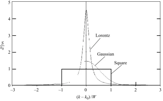
Any further progress requires us to specifyS(k). In our calculation, we have chosen the following three spectra.

(i) A square spectrum

S =s0 for k0−W < k < k0+W, (2.18)

whereW is the spectral width. (ii) A Lorentz spectrum

S = 0.09s0

[(k−k0)/W]2_{+ 0.02}. (2.19)

(iii) A Gaussian spectrum

1

–3 –2 –1 0 1 2 3

5

4

3

2

1

0

(k – k0) /W

S

Lorentz

Gaussian Square

s0

Figure 1. Three narrow spectra.

The spectra (ii) and (iii) were normalized to fulfil the following constraints: _∞

−∞

S(k) dk= 2W s0,

k0+0.9W

k0−0.9W

S(k) dk = 1.8W s0. (2.21a, b)

Equation (2.21a) guarantees that all spectra have the same total energy, and (2.21b) ensures that they have a comparable width. The three spectra are plotted in figure 1.

2.5. Growth-rate for the square spectrum

Substituting (2.18) into (2.17) and integrating over k:

1 = 8k 4 0s0 iK

arctan 2

K(γ + iW)

−arctan 2

K(γ −iW)

, (2.22)

which can be reduced to

γ2= K 2 4

4W K coth

K

8s0k04

−1

−W2. (2.23)

The right-hand side of (2.23) is real. A necessary condition for instability is Re{γ}<0, so that Im{γ}and Re{Ω}must vanish. Applying (2.12a), the growth rate is found to be

ΩI ≡Im{Ω}= K 4

g k3₀

K2 4

4W K coth

K

8s0k04

−1

−W2

. (2.24)

Defining the small steepness parameter

ε=4s0W k0=o(1), (2.25)

and the non-dimensional variables ˜

ΩI =ΩI/ε2

gk0, K˜ =K/ε k0, W˜ =W/ε k0; (2.26a–c)

(2.24) is rewritten as:

˜

ΩI = K˜ 4

˜

2.6. Growth rate for the Lorentz and Gaussian spectra

Starting from (2.19) and following a similar procedure to that outlined in the previous section, we obtain for a Lorenz spectrum

˜

ΩI = K˜ 4

2−K˜2_{/4−0.1425 ˜W. (2.28)}

The result for the Gaussian spectrum, (2.20), can only be given in an implicit form:

0.11 ˜WK˜ = Im

W

0.64 ˜K

˜

W +

5.14 i ˜ΩI

˜

WK˜

. (2.29)

The function W(z) of the complex variable z, is defined in Abramowitz & Stegun (1972, eq. (7.1.3), p. 297); it is related to the complementary error function through

W(z) = e−z2erfc(−iz). (2.30)

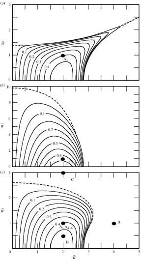
2.7. Results of linear-stability analysis

The non-dimensional growth rate ˜ΩI, see (2.26a), for the three different spectra is shown in figure 2.

Figure 2 gives nine solid isolines for each spectrum, for which ˜ΩI= 0.05,0.1,0.15, . . . ,0.45. The broken lines represent the marginal stability cases, i.e. ˜ΩI= 0. Note that ˜ΩI= 0 also on ˜K= 0. For all three spectra, the values of ˜ΩI at ˜W= 0, i.e. for non-random waves, are identical and reach a maximum ˜ΩI= 0.5 at ˜K= 2, and have

˜

ΩI= 0 at ˜K= 2√2. For the Lorentz and Gaussian spectra, the regions of instability are bounded, whereas that of the square spectrum extends to infinity, albeit with ever decreasing growth rates, along the line ˜W= 0.5 ˜K. This singular behaviour is attributed to the abrupt structure of the square spectrum. Despite the very different structure of the square and Gaussian spectra, the isolines ˜ΩI= 0.45,0.40,0.35 are surprisingly similar (see figure 3). This similarity becomes even more profound when compared to behaviour of the same isolines for the Lorentz spectrum, also given in figure 3. Note that the case of vanishing spectral width, i.e. W= 0, corresponds to the deterministic problem, for which the well-known Benjamin–Feir instability is recovered.

3. Interpretation of the initial disturbance

3.1. Spectral interpretation of the initial conditions

In (2.10), the decay rateR(r) is introduced, and there are no limitations onR except that R(0) is real and R(∞) = 0. In this section, the spectral interpretation of the inhomogeneous disturbance will be derived.

The influence of the small initial disturbance on the homogeneous spectrum can be found by dividing the spectrum in a similar way to (2.8):

S(x, k) =Sh(k) +δ S1(x, k). (3.1)

To find an interpretation forS1 we start with (2.6); by replacingS(k) withS(k, x), we obtain:

ρ(x, r, t) = _∞

−∞

exp(i(k−k0)r)

Sk, x+1 2r, t

Sk, x− 1₂r, tdk. (3.2)

1 2 3 4 5 3

2

1

0

3

2

1

0 10

8

6

4

2

0

K~ W~

W~

W~

0.1 0.2

0.3 0.4

0.1

0.2

0.3

0.4

0.1 0.2

0.3 0.4

A3

B C

D A1,A4 – 6

(c) (b) (a)

A2

Figure 2. Isolines of the non-dimensional growth-rate ˜_ΩI for three spectra: (a) square

1 2 3 4 5 3

2

1

0

W~

K~

Figure 3.Three isolines of the growth rate ˜Ω_I= 0.35,0.40,0.45, for three different spectra:

(a) ——, square spectrum; (b) – – –, Lorentz spectra; (c)· · ·, Gaussian spectra.

Using (3.1) and approximating the value under the square root in (3.2) up to order

δ:

Sk, x+1 2r, t

Sk, x−1₂r, t=Sh(k, t) +1 2δ

S1

k, x+1 2r, t

+S1

k, x−1₂r, t+o(δ2).

(3.3) Substituting (3.3) into (3.2)

ρ(x, r, t) = _∞

−∞exp(i(

k−k0)r)Sh(k, t) +1₂δS1

k, x+ 1₂r, t+S1

k, x− 1₂r, tdk.

(3.4) Equation (2.10) att= 0 gives,

ρ1(x, r) = 2R(r) cos(Kx). (3.5)

Similarly, for the spectral disturbance att= 0, we assume,

S1(x, k) = 2s(k) cos(Kx). (3.6)

Substituting (3.6) into (3.4) using (3.5) and (2.7),

2R(r) = _∞

−∞

s(k) [exp(i(k−k0+K/2)r) + exp(i(k−k0−K/2)r)] dk. (3.7)

Taking ther toχ Fourier transform of (3.7),

2 _∞

−∞

R(r) exp(−iχ r) dr = _∞

−∞

_∞

−∞

s(k) [exp(i(k−k0+K/2−χ)r)

+ exp(i(k−k0−K/2−χ)r)] drdk. (3.8)

Integrating the right-hand side overr:

1 π

_∞

−∞R(r) exp(−iχ r) dr =

_∞

−∞s(k)

δk−k0+ 1₂K−χ

+δk−k0−1₂K−χ

dk

=sk0+χ −1₂K

+sk0+χ+ 1₂K

Neglecting terms of order K2, give an equation for s(k):

s(k) = 1 2π

_∞

−∞

R(r) exp(−i(k−k0)r) dr. (3.10)

Equations (3.1), (3.6) and (3.10) give the initial spectrum.

Note the similarities between the pair (ρh(r), Sh(k)) and the pair (R(r), s(k)) as demonstrated by their interrelations:

ρh(r) = _∞

−∞

Sh(k) exp(i(k−k0)r) dk, (3.11a)

Sh(k) = 1 2π

_∞

−∞

ρh(r) exp(−i(k−k0)r) dr, (3.11b)

R(r) = _∞

−∞

s(k) exp(i(k−k0)r) dk, (3.12a)

s(k) = 1 2π

_∞

−∞

R(r) exp(−i(k−k0)r) dr, (3.12b)

3.2. Connection to the initial surface elevationη

To calculate the initial surface elevationη, we start from (2.4), (3.1) and (3.6) att= 0:

2η(x) = _∞

−∞

exp(i[kx+θ(k)])S(k, x) dk+∗

= _∞

−∞

exp(i[kx+θ(k)])Sh(k) + 2δs(k) cos(Kx) dk+∗. (3.13)

To first order inδ, (3.13) can be written:

2η= ⎡ ⎣ ∞

−∞

exp(i(kx+θ(k)))Shdk+ cos(Kx) _∞

−∞

exp(i[kx+θ(k)])

δ2_s2

Sh dk

⎤ ⎦+∗,

(3.14) which shows that the phase θ(k), of the inhomogeneous disturbance is not free, and is related to the phase of the homogeneous spectrum.

Equation (3.14) can also be written as:

2η= _∞

−∞

exp(i(kx+θ(k)))Sh(k) +1

2exp(i((k+K)x+θ(k)))

δ2_s2_(k)

Sh(k)

+ 1₂exp(i((k−K)x+θ(k)))

δ2_s2_(k)

Sh(k)

√

dk+∗. (3.15)

A shift of the integration variables in the last two terms on the right-hand side gives:

2η= _∞

−∞

exp(i(kx+θ(k)))Sh(k) +1₂exp(i(kx+θ(k−K)))

δ2_s2_(k−_K)

Sh(k−K)

+ 1

2exp(i(kx+θ(k+K)))

δ2_s2_(k+K)

Sh(k+K)

√

dk+∗. (3.16)

5

Right inhomogeneous spectrum

k0 + K

aR

a

Left

inhomogeneous spectrum

cL cR bR

aL _b

L

c

b

Homogeneous spectrum

k0 – K k0

Figure 4.Schematic description of the main homogeneous spectrum and the inhomogeneous

disturbance (hereSh(k) ands(k) are both Gaussian). As an example, the phases at (aR, bR, cR)

and at (aL, bL, cL) are the same as at (a, b, c), respectively.

4. Numerical solution of Alber’s equation

4.1. Numerical scheme

Albers equation (2.1), rewritten in terms of the following non-dimensional and stretched variables:

˜

ρ= k 2 0

ε2ρ,˜ξ=εk0

x− 1

2

g k0

t

,τ˜= (ε2gk0)t,˜r =εk0r,

reads:

i∂ρ˜

∂τ˜ + 2λ

∂2_ρ˜

∂˜ξ ∂˜r −2νρ˜

˜

ρ˜ξ+ 1₂˜r,0−ρ˜˜ξ−1₂˜r,0= 0, (4.1)

where,ν= 1/2 and λ=−1/8.

Formulating (4.1) as a finite-difference scheme, approximating the time derivative by a forward difference, and the ˜ξ and ˜r derivatives by central differences:

i

˜

ρ(n,j,+1)−ρ˜(n,j,)

τ˜

+ 2λ 4ξ ˜ ˜r

˜

ρ(n+1,j+1,)−ρ˜(n−1,j+1,)−

˜

ρ(n+1,j−1,)−ρ˜(n−1,j−1,)

−2νρ˜(n,j,)[ ˜ρ(n+j ˜r/(2˜ξ),0,)−ρ˜(n−j ˜r/(2˜ξ),0,)] = 0, (4.2) where the indexnrepresents points along the ˜ξ axis, ˜ξ=n˜ξ , n= 0,1,2, . . . , N; and

N+ 1 is the number of points along this axis. The subscriptj represents points along the ˜raxis, where ˜r=j ˜r,j= 0,1,2, . . .,M; andM+ 1 is the number of points along the ˜r axis. represents time steps where ˜τ=τ˜, = 0,1,2, . . ..

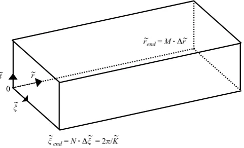
A schematic description of the domain is shown in figure 5. The numerical time-stepping scheme is formulated as follows:

˜

ρ(n,j,+1)= ˜ρ(n,j,)+

iλτ˜ 2ξ ˜ ˜r

˜

ρ(n+1,j+1,)−ρ˜(n₋1,j+1,)−

˜

ρ(n+1,j₋1,)−ρ˜(n₋1,j₋1,)

− 2i˜τ νρ˜(n,j,)[ ˜ρ(n+j ˜r/(2˜ξ),0,)−ρ˜(n−j ˜r/(2ξ˜),0,)]. (4.3) After several attempts, the following values were taken for the differential steps:

ξ˜=π/100, ˜r=π/40, and ˜τ= 2.5×10−5_{. Taking smaller values did not have a} significant effect.

4.2. Periodicity in ˜ξ

We restrict ourselves to periodic solutions in ˜ξ so that on the boundary ˜ξ= ˜ξend,

˜

0

ξ~ r

~

τ

~

ξ~end = N . ∆ξ

~ = 2π/K~

r~end= M . ∆r~

Figure 5. Schematic description of the numerical domain.

The last term on the right-hand side of (4.3) depends on values of ˜ρ at ˜

ξ= (n˜ξ+j ˜r/2) which can be larger then ˜ξend=N ξ˜. Again, the periodicity

condition is used: ˜ρ(˜ξ + 2pπ,˜r,˜τ) = ˜ρ(˜ξ ,r,˜ τ˜), where p= 1,2, . . ., or ˜ρ(n+pN,j,)= ˜

ρ(n,j,).

The values of ˜ρ along ˜r= 0, depend on points outside the domain 06˜r6˜rend.

Specifically, the second term on the right-hand side of (4.3) depends on ˜ρ(n,−1,). From

the definition of ˜ρ, (2.2), we see that ˜ρ(˜ξ ,−˜r,τ˜) = ˜ρ∗(˜ξ ,˜r,τ˜), so we can calculate the value of ˜ρ along ˜r= 0, from the condition: ˜ρ(n,−1,)= ˜ρ∗(n,1,).

4.3. Condition at large˜r

Theoretically, the ˜r axis extends to infinity, however for practical reasons, the axis must be truncated. After several attempts, the following analysis led to the boundary condition that was used for large ˜r. We start with (3.2), approximating S(k, x) by a square spectrum in (k−k0)∈(−w, w), and integrating, leads to:

ρ(x, r, t) = 2

Sx+1 2r, t

Sx−1 2r, t

sin(wr)

r . (4.4)

For r= 0: ρ(x,0, t) = 2S(x, t)w, thus S(x, t) =ρ(x,0, t)/2w; substituting back into (4.4), and switching to dimensionless quantities:

˜

ρ(˜ξ ,˜r,τ˜) =

˜

ρ˜ξ+1 2˜r,0,˜τ

˜

ρξ˜− 1 2˜r,0,˜τ

sin( ˜w˜r) ˜

w˜r , (4.5)

which is the boundary condition used at large ˜r.

The influence of the extent of the ˜r domain was checked for several values: ˜

rend= 10˜ξend, 30˜ξend and 50˜ξend. The effect of this closure is shown in figure 6, where

the maximum value of ˜ρ(˜r= 0) is presented as a function of the non-dimensional time, ˜

τ. It can be seen that all three lines are indistinguishable up to ˜τ= 17.5, (more then 300 wave periods); whereas the lines for the two larger domains overlap throughout the computation. The value of ˜r is kept constant in all cases, so the value of M is 400, 1200 and 2000, according to the increasing size of the domain.

For the case ˜rend= 30˜ξend and ˜rend= 50˜ξend, the value ˜ρmax(˜r= 0) remained at

˜

ξ= 0, ˜ξend throughout the computation (i.e. for ˜τ <35). This was also the case for

˜

rend= 10˜ξend, but only for ˜τ <17.5. Since there was no difference between ˜rend= 30˜ξend

ρ~

max (r~ = 0)

0 0.5 1.0 1.5 2.0 2.5

5 10 15 20

τ

~

25 30 35

Figure 6.The influence of the extent of the ˜_r domain on the maximum value of ˜_ρ at ˜_r= 0

as a function of non-dimensional time ˜τ, for: , ˜rend= 10˜ξend; , ˜r= 30˜ξend;䊊, ˜r= 50˜ξend. These calculations are for a homogenous Gaussian spectrum and an inhomogeneous Gaussian disturbance with ˜K= 2,W˜ = 1,δ= 0.1.

4.4. Invariants of motion

In Janssen (1983), we find that the solution to our problem satisfies certain conservation laws, and he continues to specify the first three of them. The same invariants are mentioned in Janssen (2003). Note that the existence of more than three invariants could serve as an indicator to the integrability of Alber’s equation. The first invariant which relates to the total energy is:

I1 = 2π/K

0

ρ(x,0, t) dx. (4.6)

The relative deviation ofI1 at all times from its value att= 0 did not exceeded 10−7 throughout the calculations.

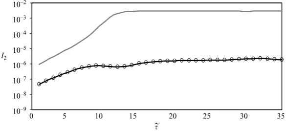
The second invariant which depends on values alongr is:

I2= 2π/K

0

_∞

−∞

κSdxdκ, (4.7)

where:

S(x, κ, t) = _∞

−∞

ρ(x, r, t)eiκr_d

r. (4.8)

Since ρ(t= 0) is real and symmetric in r; I2(t= 0) = 0. Thus, we cannot compare the values of I2 at all times to the initial value. However, an additional justification for using ˜rend= 30˜ξend, rather than ˜rend= 10˜ξend or ˜rend= 50˜ξend, can be achieved by

comparingI2 for ˜rend= 10˜ξend, ˜rend= 30˜ξend, and ˜rend= 50˜ξend. Figure 7 shows the value

ofI2 (in logarithmic scale) as a function of dimensionless time ˜τ. It can be seen that the values ofI2 for the ˜rend= 30˜ξend case are three orders of magnitude smaller then

the ones for ˜rend= 10˜ξend, and overlap the one for ˜rend= 50˜ξend.

The third invariant which depends both on the values alongr= 0, through its first term, and the values along ther axis, through its second term, is:

I3 = 2π/K

0

ρ2(x,0, t) dx−1

4 2π/K

0

_∞

−∞

κ2Sdxdκ. (4.9)

10–9

10–8 10–7

10–6

10–5 10–4

10–3 10–2

0 5 10 15 20

τ~

25 30 35

I₂

Figure 7. The influence of the extent of the_r domain on the invariant_I2 as a function of

the non-dimensional time ˜τ, for: , ˜rend= 10˜ξend; , ˜r= 30˜ξend;䊊, ˜r= 50˜ξend. Same case as figure 6.

5. Results of the numerical simulations

5.1. Description of the initial conditions

In order to apply the numerical scheme given in the previous section, the initial value of ˜ρ must be given. These initial conditions are set by (2.8) and by (2.10). It can be seen that there are several degrees of freedom. For example, the initial homogeneous distribution of ˜ρhdepends only on the initial spectrum (3.11a), which can be a square spectrum (2.18), a Lorentz spectrum (2.19), or a Gaussian spectrum (2.20). For these spectra we obtain, respectively:

˜

ρh(˜r,˜τ = 0) = sin( ˜W˜r)

2 ˜W˜r , (5.1)

˜

ρh(˜r,˜τ = 0) = 0.9π

4√2exp(−0.1˜r ˜

W√2), (5.2)

˜

ρh(˜r,˜τ = 0) = 1.133 √

π

4 exp(−((˜rW˜)

2_{/6.45)). (5.3)}

These correlation functions depend on one free parameter ˜W.

From (2.10), we can see that the value of the inhomogeneous disturbance wave number ˜K, and the inhomogeneity parameter δ are also free quantities. The decay rate ˜R(˜r) that appears in (2.8) is also free; however one could choose the initial inhomogeneous spectral disturbance, and then use (3.12a) to calculate ˜R(˜r).

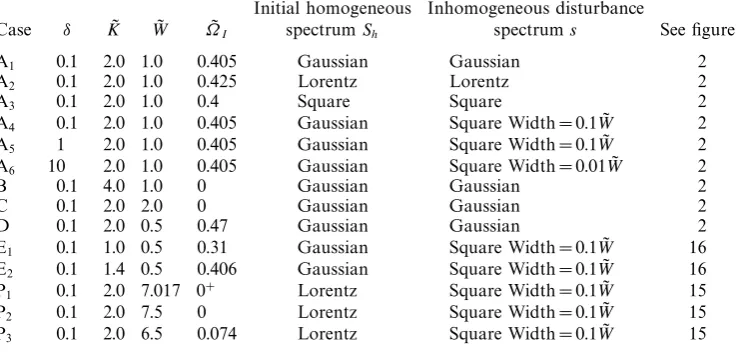
The influence of various initial conditions will be discussed in this section. The different cases studied are summarized in table 1 and marked by dots in figures 2, 15 and 16.

5.2. Reference case (A1)

The chosen reference case is unstable, its initial homogenous and inhomogeneous spectra are Gaussian with ˜W= 1.0. ˜K= 2.0, and the small inhomogeneous parameter

δ= 0.1.

Initial homogeneous Inhomogeneous disturbance

Case δ K˜ W˜ Ω˜I spectrumSh spectrums See figure

A1 0.1 2.0 1.0 0.405 Gaussian Gaussian 2

A2 0.1 2.0 1.0 0.425 Lorentz Lorentz 2

A3 0.1 2.0 1.0 0.4 Square Square 2

A4 0.1 2.0 1.0 0.405 Gaussian Square Width = 0.1 ˜W 2

A5 1 2.0 1.0 0.405 Gaussian Square Width = 0.1 ˜W 2

A6 10 2.0 1.0 0.405 Gaussian Square Width = 0.01 ˜W 2

B 0.1 4.0 1.0 0 Gaussian Gaussian 2

C 0.1 2.0 2.0 0 Gaussian Gaussian 2

D 0.1 2.0 0.5 0.47 Gaussian Gaussian 2

E1 0.1 1.0 0.5 0.31 Gaussian Square Width = 0.1 ˜W 16

E2 0.1 1.4 0.5 0.406 Gaussian Square Width = 0.1 ˜W 16

P1 0.1 2.0 7.017 0+ Lorentz Square Width = 0.1 ˜W 15

P2 0.1 2.0 7.5 0 Lorentz Square Width = 0.1 ˜W 15

P3 0.1 2.0 6.5 0.074 Lorentz Square Width = 0.1 ˜W 15

Table 1. Summary of parameters chosen for the various simulations.

0 0.5 1.0 1.5

ρ~ (ξ~, 0,τ~) 2.0 2.5

0.5 1.5

ξ~

1.0 2.0 2.5 3.0

Figure 8.The value of ˜ρas a function of ˜ξ, at ˜r= 0 for different times: , ˜τ= 0;

, ˜τ= 8.25; , ˜τ= 16.25;䊊, ˜τ= 24.5. case A1.

case where most of the energy is concentrated at the two ends of the region at ˜

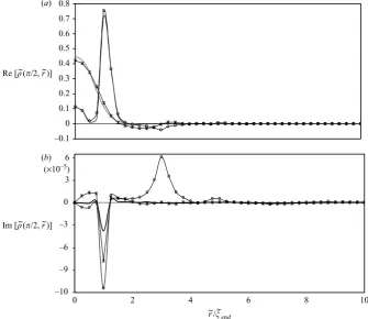
τ= 8.25, and back to (almost) the initial distribution of ˜ρ at ˜τ= 16.25 (for ˜τ= 24.5, the picture returns to that of ˜τ= 8.25). In figure 9(a), the real part of ˜ρas a function of ˜r at ˜ξ= ˜ξend/2, is plotted as a function of ˜r/˜ξend for the same times as appear

in figure 8. It can be seen that the values of the real part of ˜ρ are nearly identical for ˜τ= 0, ˜τ= 16.25, and also the values at ˜τ= 8.25 and ˜τ= 24.5 are the same. In figure 9(b), the imaginary part of ˜ρ at the same cross-section is plotted, recurrence is less evident. Note that the magnitude of the real part is ten thousand times larger than the magnitude of the imaginary part.

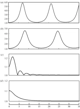
5.3. The influence of the initial linear growth rate on the long-time evolution

In figure 10, the long-time evolution of ˜ρ(0,0,˜τ)/ρh˜(0) is presented for the cases A1, B, C, D (see figure 2c). In all of these cases, the starting homogeneous, and the inhomogeneuos disturbance spectra were Gaussian, and the inhomogeneity parameter

–0.1 0 0.1 0.2 0.3 0.4 0.5 0.6 0.7 0.8

–10 –9 –6 –3 0 3 6 (×10–5) (b) (a)

0 2 4 6 8 10

Re [ρ~(π/2, r~)]

Im [ρ~(π/2, r~)]

r

~/ξ~end

Figure 9. The values of (a) the real part of ˜ρ and (b) the imaginary part as a function of

˜

r/˜ξend, at the cross-section ˜ξ= ˜ξend/2, for different times. , ˜τ= 0; , ˜τ= 8.25; , ˜τ= 16.25; , ˜τ= 24.5. case A1.

homogeneous value. It can be clearly seen from figure 10 that the value of ˜ρ(0,0,τ˜) increases to 5.8 times the initial homogenous value for case D, which is the most unstable case treated here, with a growth rate of 0.47. In case A1, which is unstable and its growth rate is 0.405, this value increases to 4.5 times the initial value. For the third and fourth cases that appear in figure 10, the corresponding points in figure 2c

are in the stable region. Case C which has the same ˜K as case A1, but ˜W is 3 times larger, initially increases to 1.25 of the initial homogeneous value, and oscillates with decreasing value to the initial homogeneous value. The fourth case, B, in which the spectrum has the same ˜W as case A1, but the wavenumber of the disturbance ˜K is doubled, decreases monotonically to the initial homogeneous value.

5.4. Influence of the shape of the initial spectrum

Figure 11 illustrates the long-time evolution of ˜ρ(0,0,˜τ)/ρh˜(0) for the three different initial homogenous spectra Sh(k), described in §2, when the small inhomogeneous disturbance spectrum s(k) has the same structure as the homogeneous one, and the inhomogeneity parameter is δ= 0.1. These cases are marked as A1, A2, and A3 in figure 2. Figure 11 demonstrates the difference between the Gaussian spectrum, the square spectrum and the Lorentz spectrum. As we can see, the maximal value of

˜

0

0 5 10 15 20 25 30 35

6.0 (a)

(b)

(c)

(d) 5.0 4.0 3.0 2.0 1.0 5.0 4.0 3.0 2.0 1.0

1.2

1.1

1.0 1.2

1.1

1.0

0 5 10 15 20

τ

~

25 30 35

Figure 10. The value of ˜ρ(0,0,˜_τ)/_ρ˜_h(0) as a function of time, for four different initial

growth rates, cases (a) D, (b) A1, (c) C and (d) B of figure 2(c) and table 1.

We can see from table 1 that indeed its growth rate is also greater, for the same initial ˜W and ˜K. Besides the maximal value, the differences are relatively small, and in particular, the period of the recurrence for the three spectra is similar.

5.5. Influence of the shape of the inhomogeneous disturbance

The influence of the shape of the inhomogeneous disturbance is checked for four different cases.

(i) The reference case with Gaussian homogenous and inhomogenuos disturbance spectra (case A1).

(ii) Gaussian homogenous spectrum with a small square inhomogenuos disturbance,

δ= 0.1, and the width of the spectrum s(k) is 10% of the width of Sh(k), as shown schematically in figure 12 (case A4).

1 2 3 4 5

0 5 10 15

τ

~

20 25 30 35

Figure 11. The values of ˜ρ(0,0,˜τ)/ρ˜_h(0) as a function of time for three different initial

spectra: , square (A1); 䊐, Gaussian (A3); , Lorentz (A2).

k0

s0

10s0

k0 + K

k0 – K

Figure 12. Schematic description of the initial homogenous spectrum and the

inhomogeneous disturbances, , case A4; , case A5; , case A6.

(iv) Case A6 for which the width of the disturbance is 0.01 ˜W but δ= 10, so that the total area under the disturbance spectra is the same as in case A5.

In figure 13, the value of ˜ρ(0,0,τ˜)/ρh˜ (0) is shown. It can be seen that although the inhomogenuos disturbance is different from case to case the maximum value of

˜

ρ(0,0,τ˜)/ρh˜(0) is the same, and seems to depend only on the initial homogenous width ˜

W , and the disturbance wavenumber ˜K. However, owing to the weak disturbance in case A4 the period of recurrence is much larger, as was shown by Stiassnie & Kroszynski (1982) for the deterministic problem. Despite the difference in the disturbance width between cases A5 and A6, the values of ˜ρ(0,0,τ˜)/ρh˜(0) are nearly identical, probably because the energy of the disturbance is the same in both cases.

6. Discussion

1 2 3 4 5

0 5 10 15

τ~ 20 25 30 35

Figure 13.The values of ˜ρ(0,0,˜τ)/˜ρ_h(0) as a function of time, for four different initial

inhomogeneous disturbance spectra:×, Case A1; , Case A4; , Case A5;䊊, Case A6.

1.00 1.04 1.08 1.12 1.16 1.20

0 20 40 60

τ~ 80 100

Figure 14. The value of ˜ρ(0,0,˜τ)/˜ρ_h(0) as a function of time for three cases near the

threshold of instability. , P1; , P2;䊐 䊐, P3.

As mentioned in §1, the only known attempt to obtain subsequent evolution for the solution of Alber’s equation, is that of Janssen (1983). Janssen used an asymptotic method to solve the problem near the threshold of instability and obtained a solution which is characterized by an initial small overshoot followed by an oscillation around its time-asymptotic value. In figure 14 we present results of the behaviour of our numerical solution near and at the threshold of instability for the case of an initial Lorentz spectrum with a small square disturbance, for ˜K= 2.0 and ˜W= 6.5, 7.017 and 7.5. These three cases are marked in figure 15 as P3, P1 and P2, respectively. The results in figure 14 for the cases P1 and the P2 are similar to what one would expect from Janssen’s description of his asymptotic approximation. Note that the result for P3is recurring with a rather long recurrence-period (the period is approaching infinity as we approach the marginal stability line from below).

Note that the numerical recurrence demonstrated by our results finds some support in Janssen (1983). He defines W(x, p, t), (given by the r to p Fourier-transform of

30 10

8

6

4

2

0

W~

0.1

0.2

0.3 0.4

1 2 3 4 5

K~

P2

P1

P3

Figure 15. Three cases near the marginal-stability curve, see table 1.

1 2 3 4 5 3

2

1

0

K W

~ ~

0.1 0.2

0.3 0.4

0.1

0.2 0.3

E1

A4

E2

Figure 16.The distinction between cases of simple and complex recurrence.

this transport equation turns out to be invariant under the transformation t→ −t.

p→ −p, indicating, in our opinion, that the energy transfer (owing to the spatial inhomogeneities) is possibly reversible. However, it turns out that the above condition is probably necessary, but not always sufficient. To demonstrate this we have chosen cases for which 2 ˜K are also within the unstable region, see points E1 and E2 in figure 16. This property is shared by all points within the shaded zone in figure 16. From figure 17, we can see that the graphs for cases E1, E2 are very different from that of A4, they are not recurring. The growth rate of A4is equal to that of E2 which is larger than that of E1; however, the value of ˜ρmax is larger for E2 than for A4, and

largest for E1. (˜ρmax is the maximum value that ˜ρ(˜ξ ,0,τ˜) obtains for a fixed ˜τ, and

˜

ξ ∈(0,˜ξend), for complex recurrence the maximum value is moving and does not stay at ˜ξ= 0 any more.) This could be explained from the values of the growth rates of 2 ˜K disturbances, which are 0.48, 0.23 and 0 for cases E1, E2 and A4, respectively. We call this type of behaviour ‘complex recurrence’, adopting the terminology of Yuen & Ferguson (1978) who have obtained analogous results for the Schr¨odinger equation.

2 4 6 8

0 10 20 30 40 50 60 70

τ

~

Figure 17.The value of ˜_ρmax/˜_ρh(0) as a function of time for two cases in the complex

recurrence zone, E1 and E2, and a case in the simple recurrence zone A4, see table 1. , E1;

, E2; , A4.

The question about the possible manifestation of such inhomogeneous disturbances in nature is crucial for the physical feasibility, not only of the newly calculated evolutions, but also for Alber’s (1978) linear stability analysis.

One possible mechanism to generate such disturbances is related to sea-swell interaction, for which the coexistence of a narrow-banded random sea and of a monochromatic swell of much larger wavelength, is assumed.

The superharmonics and subharmonics which are generated by their interaction (which are rather close to free waves), can probably serve as the inhomogeneous disturbances, very similar in nature to those described in§3.

Janssen (2003) applied a Monte Carlo approach to a naive discretization of Zakhaov’s equation, using random initial phases, and obtained an irreversible widening of the spectrum. Similar results were also found by Dysthe et al. (2003) who have used the modified Schr¨odinger equation with random initial phases. It seems plausible that recurrence could be recovered by their approaches, provided that appropriate initial phase-relations are used. The overall averaged spectrum calculated from our computations resembles the irreversible Monte Carlo results. This overall spectrum is

¯ ¯

S(k) = 1

T

T

0 ¯

S(k, t) dt, (6.1)

whereT denotes the recurrence time, and ¯S(k, t) is the space-averaged spectrum:

¯

S(k, t) = K 2π

2π/K

0

S(k, x, t) dx. (6.2)

S(k, x, t) in (6.2) is inspired by (47) to (50) of Crawford et al. (1980), and given by

S(k, x, t) = 1 2π

_∞

−∞

ρ(x, r, t) exp(−i(k−k0)r) dr. (6.3)

In figure 18(a) we give ¯S¯(k)/Sh(0) and compare it to Sh(k)/Sh(0) for the case A1. In figure 18(b) we show ¯S(k, t)/Sh(0) att= 0,t=T /4,t=T /2. The curve atT =T /2 demonstrates an almost equal partition of the energy between the base spectrum and the disturbances. The area under the graph of ¯S¯(k)/Sh(0) in figure 18(a) is 0.6% larger than that under ¯S(k, t)/Sh(0) att= 0.

1.0 0.8 0.6 0.4 0.2

0

–0.4 –0.2 0 0.2 0.3 (k – k0)/k0

1.0 0.8 0.6 0.4 0.2

0 (a)

(b)

Figure 18. (a) The overall averaged spectrum , ¯S(k)/S¯ _h(0); compared to ,S_h(k)/S_h(0).

(b) The spatial averaged spectra , ¯S(k, t)/Sh(0) fort= 0;䊊 䊊,t=T /4; ,t=T /2.

future. The extension to broad spectra is a much more complicated issue, and it still awaits the development of an appropriate model equation. In this respect, we should mention preliminary attempts to study sea-states governed by a system, of two Alber’s equations, such as in Stiassnie (2001) and Shukla, Markland & Stenflo (2006).

Note that the time scales involved in the recurrence are much shorter than those of the kinetic equation. We can say that the choice of overall random phases in the derivation of the kinetic equation, which results in longer time-scales also ‘average out’ the recurrence phenomenon. The kinetic equation is the main tool for calculating nonlinear interaction in wave-forecasting models, see Komen et al. (1994), and it will probably remain so for some time to come. However, model equations, such as Alber’s equation can be helpful when addressing phenomena governed by smaller time/space scales, such as the development of freak waves.

This research was supported by The Israel Science Foundation (Grant 695/04) and by the US–Israel Binational Science Foundation (Grant 2004-205). The authors are grateful to Dr A. Zuevsky for his help in the early stages of this work.

R E F E R E N C E S

Abramowitz, M. & Stegun, A.1972Handbook of Mathematical Functions. Dover.

Alber, I. E.1978 The effects of randomness on the stability of two-dimensional wavetrains.Proc.

R. Soc. Lond.A363, 525–546.

Annenkov, S. Y. & Shrira, V. I.2006 Role of non-resonant interactions in evolution on nonlinear

Crawford, D. R., Saffman, P. G. & Yuen, H. C.1980 Evolution of a random inhomogeneous field

of nonlinear deep-water gravity waves.Wave Motion 2, 1–16.

Dysthe, K. B., Trulsen, K., Krogstad, H. E. & Socquet-Juglard, H. 2003 Evolution of a

narrow-band spectrum of random surface gravity waves.J. Fluid Mech.478, 1–10.

Hasselmann, K.1962 On the non-linear energy transfer in a gravity-wave spectrum. Part 1. General

theory.J. Fluid Mech.12, 481–500.

Janssen, P. A. E. M. 1983 Long-time behaviour of a random inhomogeneous field of weekly

nonlinear surface gravity waves.J. Fluid Mech.133, 113–132.

Janssen, P. A. E. M.2003 Nonlinear four-wave interaction and freak waves.J. Phys. Oceanogr.33,

863–884.

Kinsman, B.1965 Wind waves, their generation and propagation on the ocean surface. Prentice-Hall. Komen, G. J., Cavaleri, L., Donelan, M., Hasselmann, K., Hasselmann, S. & Janssen, P. A. E. M.

1994Dynamics and Modelling of Ocean Waves. Cambridge University Press.

Shukla, P. K., Markland, M. & Stenflo, L.2006 Modulational instability of nonlinear interacting

incoherent sea states.Sov. Phys., J. Exp. Theor. Phys. Lett.84, 645–649.

Stiassnie, M.2001 Nonlinear interaction of inhomogeneous random water wave.ECMWF Report

of the Workshop on Ocean Waves Forecasting, Reading, July 2–4, pp. 39–52.

Stiassnie, M. & Kroszynski, U. I. 1982 Long time evolution of an unstable water-wave train.

J. Fluid Mech.116, 207–225.

Yuen, H. C. & Ferguson, W. E.1978 Relationship between Benjamin–Feir instability and recurrence

in the nonlinear Schr¨odinger equation.Phys. Fluids 21, 1275–1278.

Zakharov, V. E.1968 Stability of periodic waves of finite amplitude on the surface of a deep fluid.