*Corresponding author. Fax:#972-4-822-1529. E-mail address:[email protected] (R. Linker)
Robust controllers for simultaneous control of temperature
and CO
concentration in greenhouses
R. Linker*, P.O. Gutman, I. Seginer
Agricultural Engineering Department, Technion, Haifa, 32000 Israel
Received 13 March 1998; accepted 12 March 1999
Abstract
The present work focuses on the control of greenhouse air temperature and CO
concentration by means of simultaneous
ventilation and enrichment. Such an operation, which may a priori seem contradictory, was shown by several authors to be required to maintain optimal temperature and CO
setpoints. The control process is divided into two distinct control loops, the "rst maintaining the temperature by adjusting the ventilation, and the second maintaining the CO
concentration by adjusting the
enrichment. The CO
concentration controller assumes the ventilation rate to be constant and approximately known over 2-min
intervals. Implementation in an experimental greenhouse shows the ability of the controllers to meet the requirements. 1999 Elsevier Science Ltd. All rights reserved.
Keywords: Greenhouse; Robust control; Neural network; Optimal climate
1. Introduction
It has been known for years that, in addition to tem-perature and solar radiation, the COconcentration of the air has a direct in#uence on crop photosynthesis (e.g.
Idso and Idso, 1994). CO
enrichment, which consists of supplying highly concentrated CO
to the greenhouse, is a daytime procedure widely used in greenhouses to in-crease crop yield (e.g. Kimball, 1986). However, in warm climates, ventilation is required during most of the day to lower the temperature, and a con#ict exists between the
need to ventilate and the desire to enrich. While common practice usually views ventilation and enrichment as mu-tually exclusive, several studies related to optimal green-house control under warm climates (Ioslovich et al., 1995; Linker et al., 1998; Seginer et al., 1986) have shown that in order to maintain, at any time, optimal temperature and CO concentration, simultaneous ventilation and enrichment would be required.
While a wide range of greenhouse climate controllers have been described in the literature, these were not designed speci"cally in order to enable simultaneous use
of ventilation and enrichment. The documented
control-lers range from switching logics (Chao and Gates, 1996) to an improved digital PI controller (Chotai et al., 1991), and LQI controllers (Nishina et al., 1997). Feedforward control has also been studied, especially in connection with greenhouse heating (Davis and Hooper, 1991; Takakura et al., 1994). Because of the di$culty of
obtaing accurate models, adaptive control has also been in-vestigated (Boaventura Cunha et al., 1997; Sigrimis and Rerras, 1996). In the present work, robust feedback con-trollers are used to deal with the modeling errors (so-called`uncertaintiesa). A combination of robust feedback and adaptive feedforward from the disturbances has also been studied (Linker, 1995), but is not described here due to space limitations.
2. Materials and methods
The data required to design the controllers were col-lected in a single-span, pitched-roof greenhouse at the Technion, Haifa, Israel. The greenhouse had a 8 m by 6 m#oor, with a volume of 190 m, the long axis pointing
northeast. No crop was present in the greenhouse at the time of the experiment, but the concrete#oor was
con-tinuously wetted to simulate a greenhouse with a wet soil surface. Therefore, the results presented here are sup-posed to apply to a greenhouse with small seedlings
Nomenclature
c speci"c heat of air at constant pressure,
J/(kg[air]K) D wind direction, deg
F level of speed of the fans, dimensionless H e!ective height of the greenhouse, m h absolute humidity, kg[vapor]/kg[air] O opening of screen, %
Q ventilation#ux, m/(m[ground]s) q shift operator, dimensionless
R CO
#ux, kg[CO
]/(m[ground]s) s Laplace operator, 1/s
S solar radiation#ux, W/m[ground] ¹ temperature, K
t time, s
u control variable de"ned by Eq. (8), W/m
; overall heat transfer coe$cient of cover,
W/(m[ground]K) = wind speed, m/s
X CO
concentration of air, kg[CO]/kg[air]
Greek letters
* delay in the COcontrol loop, s
j latent heat of vaporization of water, J/kg[vapor]
" solar heating e$ciency, dimensionless
o air density, kg[air]/m
h indoor}outdoor temperature di!erence, K
# time average ofh, K
m indoor}outdoor CO
concentration di!erence, kg[CO
]/kg[air]
Subscripts 1 large fan 2 small fan des desired FB feedback
i inside greenhouse nom nominal
o outside greenhouse r reference
s sampling
Superscript opt optimal
Acronyms FB feedback NN neural network
RMS root mean square, de"ned in Eq. (4)
R coe$cient of linear correlation, de"ned in
Eq. (5)
which do not in#uence the greenhouse climate but
re-quire CO
enrichment. The experimental setup has been fully described in a separate paper (Linker et al., 1998), and only the elements relevant to the present study are brie#y described below.
The variables measured in the greenhouse included dry bulb and wet bulb air temperature, and CO
concentra-tion. The outside weather measurements consisted of dry bulb and wet bulb air temperature, solar radiation, and wind speed and direction.
The greenhouse climate control variables consisted of CO
enrichment and forced ventilation. Since this study focused on daytime control under summer conditions, heating was not considered. Two variable-speed fans (extracting the air from the greenhouse) were mounted on the southwest wall. The fans were rated at 3.39 and 0.46 m/s. The discharge ranges of the fans were dis-cretized. The large fan had eight equally spaced operating levels, each increment being slightly smaller than the full capacity of the small fan. The range of the small fan was divided equally into four levels. Altogether, 32 distinct operating levels were possible (labeled 0}31). The control
variablesF
andFrepresent the levels of operation of the large and small fans, respectively. A linear combina-tion of these two variables, namelyF"4F
#F
is also used below. An 80 cm wide opening, spanning the whole length of the northeast wall of the greenhouse, was con-structed. The opening could be obstructed to any degree by a motorized screen, unfolding from the top. In order to achieve"ne control at low ventilation rates, the lower
part of the opening was partly obstructed by solid tri-angles. Ten equally spaced screen positions (every 8 cm), represented by the control variableO, were allowed. Pure CO
from pressurized containers was injected at the four corners of the greenhouse, through an electrically con-trolled valve. The injection rate, 1.78;10\kg[CO
]/s, was calculated from di!erential weighing of the CO
container.
Measurements relative to greenhouse climate and out-side weather were recorded by two separate data loggers. Both data loggers were connected to a Personal Com-puter (PC) which determined the setpoints and control signals. All measurements were performed every second, except for the screen position, which, in order to be accurate, had to be measured more frequently, once every 0.15 s. 10-min averages of the weather measurements and 2-min averages of the greenhouse climate were transmit-ted to the PC. Due to hardware limitations, the control variables were computed only every 2 min, based on averages of the measurements made during the preceding 2 min. Fan operating levels and the screen opening were maintained constant over 2 min intervals, while an ap-proximately constant enrichment rate was achieved by pulse-width modulation: the CO
Fig. 1. Greenhouse optimal control scheme.Qis the ventilation rate,Ris the enrichment rate,¹
Gis the greenhouse air temperature, andXGis the CO concentration.
3. Control-system architecture
Fig. 1 presents a general scheme of greenhouse optimal control, which includes three decision levels (e.g. Tantau, 1991). The global optimization (highest decision level), which considers the whole growing season and produces costate variables, has been treated, for instance, by Seginer et al. (1991), and van Henten (1994). The inter-mediate level, which performs a local optimization, was described, among others, by Gutman et al. (1993), Bailey and Chalabi (1994), and Linker et al. (1998). The local optimization, which can be performed several times an hour, provides either optimal actuator positions or opti-mal setpoints for the controlled variables. In the second case, the setpoints have to be maintained by the lowest control level, on which the present paper focuses.
As mentioned in the previous section, the means of action on the greenhouse climate are the speeds of the
two fans, the opening of the screen, and the rate at which CO
is injected. The latter in#uences only the CO
con-centration, while the"rst two determine the ventilation
rate (Q), which in#uences both the temperature and the
CO
concentration. These observations lead to the fol-lowing schematic form, where;denotes a linear or non-linear dependence (adapted from Ioslovich et al., 1995).
d¹ G/dtdX G/dt
"
;0
0 ;
¹ G
XG#
; 0
; ;
Q
R
#
; ; ;0 ; 0
¹ M S
M h
G!h M
. (1)
The "rst vector on the right-hand side contains the
state variables (inside air temperature ¹
G, and CO concentration,X
[image:3.596.289.485.591.673.2]Fig. 2. Cascaded controller for the simultaneous control of temper-ature and COconcentration.Qis the ventilation rate,Ris the enrich-ment rate, ¹
G is the greenhouse air temperature, XG is the CO concentration, and¹
G andXG denote the optimal setpoints.
variables (ventilation rate, Q, and enrichment rate, R), and the third one represents the disturbances, which, in the present case, are measured (solar radiation,S
M,
out-side air temperature,¹
M, and inside and outside
humid-ity, h
G and hM). Note that this simple representation
assumes that heat storage takes place in the greenhouse air only (and not in the structure).
The system described by Eq. (1) can be controlled by two decoupled loops (Fig. 2):
1. A temperature loop which determines the ventilation rate.
2. A CO
loop which determines the COenrichment, for a given ventilation rate.
A direct consequence of this architecture is that venti-lation is not used to lower a CO
concentration that is higher than the setpoint. This sometimes causes the CO
concentration to present overshoots for prolonged peri-ods of time. However, since a higher CO
concentration has always a positive e!ect on photosynthesis, lowering
the CO
concentration by ventilating would be wasteful. The manipulated variable &ventilation rate' Qis
con-trolled through the fan speeds (F and F) and screen opening (O). Since this control variable is not measurable on-line, a model relating the position of the actuators to the resulting ventilation rate is needed. Such a model is presented in the next section.
4. Ventilation rate modeling
A neural network (NN) was trained to predict the ventilation rate from the control variables (F
,F, and
O), and the measured disturbances (wind speed, =and direction, D). The data required to train such a model were obtained through gas decay tests (e.g. Nederho!
et al., 1984) for which, since no crop was present in the greenhouse, COcould be used as a tracer gas. At the beginning of each test, CO
was introduced into the unventilated greenhouse until a prespeci"ed CO
level was reached. After stopping the enrichment, the ac-tuatorsF
,FandOwere set to the desired level, and the resulting exponential decrease of CO
concentration was used to determine the ventilation rate o!-line, using the
following simple"rst-order model:
oHdXG
dt "!oQ(XG!XM), (2)
whereHis the e!ective height of the greenhouse (3.5 m),
andois the air density (1.2 kg/m). Assuming the outside CO
concentration XM and the ventilation rate Q (i.e.,
indirectly wind speed and direction) to be constant, inte-gration of Eq. (2) leads to
(XG(t)!X M)"(X
G(0)!X
M)e\/R& (3)
which can be used to determineQgraphically.
A neural network having as inputs wind speed and direction, fan speeds, and screen opening, and as output the ventilation rate, was trained using the Matlab Neural Networks Toolbox (Demuth and Beale, 1992). The neu-ral network had one hidden layer of two nodes with sigmoid activation functions, and a linear output layer. Altogether, 195 tests were available, of which 174 were used as a training set, and 21 as a testing set. Table 1 presents the training and testing results in terms of the root mean square (RMS) of the residual error, and in terms ofR, the coe$cient of linear correlation between
the measured and predicted values. The error RMS is de"ned as
RMS" H
(y
H!y
H ), (4)
whereyHdenotes thejth data-point, andyH denotes the NN prediction for the corresponding data point. The coe$cient of linear correlationRis de"ned as
R"1! H(yH !>
H)
H(yH!y) (5)
wherey denotes the average of they
H's, and >
H denotes
the jth prediction of a linear regression between the measured and NN predicted values.
The results in Table 1 show the ability of the NN to model the ventilation rate. Adding hidden nodes did not improve the performance of the NN. The NN predictions are presented graphically in Fig. 3. The decrease of the predicted ventilation rate each time that the small fan is turned o!and the large fan level is increased, means that
Fig. 3. Ventilation neural-network model predictions.Dand=are the wind direction and speed, respectively.Fis the fan speeds, andQis the predicted ventilation rate. In each graph, each curve corresponds to a di!erent screen opening. The upper curves correspond to a fully opened screen,
[image:5.596.120.438.419.674.2]the lower ones to closed screen.D"0 corresponds to wind blowing in the&screen-to-fans'direction. Table 1
Neural-network ventilation model: performance over the training and testing sets (maximum ventilation rate: 50;10\(m/(ms)). Ventilation NN
Rtraining 0.92
RMS training (m/(ms)) 0.0012
Rtest 0.95
RMS test (m/(ms)) 0.0008
than the discharge due to one additional step of the large fan. This overlap ensures that the ventilation rate can be controlled continuously. A comparison between ventila-tion rates predicted with similar actuator posiventila-tions, but di!erent wind speed and direction, shows wind in#uence.
Wind speed has only a limited in#uence, but wind
direc-tion signi"cantly in#uences the ventilation rate. Using
the situation of a wind blowing in a direction perpendicu-lar to the screen-to-fans direction (D"903) as reference,
it may be seen in Fig. 3 that wind blowing in the screen-to-fans direction (left"gures,D"03) increases the
venti-lation rate. The wind e!ect is larger at small ventilation
rates, which leads to the slightly convex pictures. Sim-ilarly, wind blowing in the direction opposite to the forced ventilation (right "gures, D"1803) reduces the
ventilation rate. Here too, the wind in#uence is larger at
small ventilation rates; hence the concave graphs.
5. Temperature controller
5.1. Robust controller design
In order to design the temperature controller, the fol-lowing "rst-order energy balance model of the
green-house is used:
ocHd¹G
dt""SM!(ocQ#;)(¹G!¹M)!ojQ(hG!hM),
(6)
wherecis the speci"c heat of air (1005 J/(kg K)),;is the
overall heat transfer coe$cient of the cover,"is the solar
heating e$ciency, andjis the latent heat of vaporization
of water (2.5;10 J/kg(vapor)). In this model, the left-hand side term describes the sensible heat rate of change, the "rst term on the right-hand side denotes the solar
energy#ux absorbed by the greenhouse, the second term
the heat#ux leaving the greenhouse by ventilation and
through the cover, and the third term describes the latent heat exchange.
The solar radiation heating e$ciency (") was
deter-mined using data with maximum ventilation rate, so that the heat transfer through the cover (characterized by;) could be ignored. Afterwards, the overall heat transfer coe$cient of the cover (;) was determined using data
with very low ventilation rate. This identi"cation led to
Fig. 4. Temperature control loop.
; can be explained by the simplicity of the model (Eq. (6)), which, for instance, does not include the heat storage in the#oor and the greenhouse structure. Such
unmodeled e!ects appear as uncertainty in the existing
parameters. Note that since the parameter "enters the model only through a measured disturbance, its actual value is not important for the design of the controller.
The controller based on this model determines the required ventilation rate, which is translated into fan speeds and a screen opening using the NN model pre-sented in the previous section (Fig. 4). Since there are three actuators (large and small fan speeds, and screen opening), and only one controlled variable,Q, the same ventilation rate can be obtained with di!erent
combina-tions of the actuators. Therefore, it has to be decided a priori which combination will be considered as best. Based on mechanical considerations, it was decided to try to reduce changes in the fan speeds. In order to do so, a "rst search over the screen opening is performed in
order to determine if the desired ventilation rate can be obtained by adjusting the screen opening alone. If this is not the case, a new search is performed over the screen opening, assuming di!erent speeds for the small fan. If
the desired ventilation rate can still not be attained, the whole procedure is repeated with all the possible speeds for the large fan. Since the desired ventilation rate cannot be exactly realized, a di!erence of 10\ m/(ms)
be-tween the desired and predicted values is considered acceptable.
Due to the bi-linearity of the model (6) (term Q¹ G),
linear control methods may not be suitable. However, the structure of the non-linearity makes it suitable for feed-back linearization (Gutman, 1981). Assuming that the inside and outside temperatures and humidity do not change over a 2-min interval, Eq. (6) can be rewritten as
ocHdh
dt""SM!;h!u, (7)
where
u"ocQh#ojQ(h G!h
M) (8)
and
h"¹ G!¹
M. (9)
Considering the solar radiation as a disturbance, Eq. (7) gives the following di!erential equation linkinguandh:
dh
dt"Ah#Bu (10)
withA"!;/(ocH) andB"!1/(ocH). Since the
con-trol variables are changed only every 2 min, the model has to be discretized into the following form:
h((k#1)t
Q)"eRQh(kt Q)#
RQ
eTdvBu(kt
Q) (11)
"eRQh(kt Q)#1
A(eRQ!1)Bu(ktQ), (12)
wheret
Q is the sampling time (120 s). The control
vari-ables are determined using 2-min averages and not instantaneous measurements, so that the controlled variable is
H((k#1)t Q)"1
tQ
RQ
h
(ktQ#v) dv (13)
"1 t
Q
eRQ!1
A h(ktQ)#
B A
eRQ!1!At Q
A u(ktQ)
.
(14)
Eliminating husing Eq. (12), and introducing the shift operatorq,
H(q)" B
At
Q
(eRQ!1!At
Q)q#(1!eRQ#At QeRQ)
q(q!eRQ) u(q).
(15)
This model includes one parameter which is only approx-imately known,;(;3[3; 10]). Furthermore, the actual
ventilation rate is not exactly the desired one and, based on the performance of the NN ventilation model present-ed in Section 4, as well as rapid changes in wind spepresent-ed and direction, an uncertainty of$10% inQ was
con-sidered (Q3 [0.9; 1.1]Q
), leading to
H(q)" B
AtQ
(eRQ!1!At
Q)q#(1!eRQ#At QeRQ)
q(q!eRQ) iu(q)
(16)
"P(q)iu
(q) (17)
withi3[0.9; 1.1].
Due to the modeling uncertainties, robust control could be used, and Horowitz's method (Horowitz and
Sidi, 1972; Gutman et al., 1988) was chosen. In this method, the designer speci"es time-domain speci"cations
which are translated into frequency-domain ones, using a second- or third-order model for the closed-loop sys-tem. Based on these speci"cations and the model
uncer-tainties, the Horowitz bounds are created in the Nichols chart (which allows one to read closed-loop performance from the open-loop gain and phase). These bounds de"ne
Fig. 5. Temperature model value sets.
Fig. 6. Temperature control loop. Nominal open-loop (Eqs. (17) and (18)) and Horowitz bounds at design frequencies.
closed-loop system meets the speci"cations and is stable.
The method ends with the design of a pre"lter.
In the present case, a compromise between the limita-tions imposed by the sampling frequency and the desire to achieve tight control leads to the following reference step response speci"cations: maximum overshoot 20%,
rise time (80%) 240}600 s, settling time ($10%) 960 s.
Following Horowitz's method, these time-domain
speci-"cations are translated into frequency-domain speci"
ca-tions, and, in order to ensure stability of the closed loop, a sensitivity speci"cation of 6 dB is also introduced.
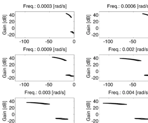
In order to proceed with the design of the controller, the value sets (e.g. Barmish, 1988), which describe the model uncertainty in the Nichols chart, have to be com-puted. Following AsstroKm and Wittenmark (1994), the
mappingq"exp( jut
Q) is used inP(z)i (Eq. (17)) for all
combinations of;andi, leading to the value sets pre-sented in Fig. 5.
Combining the frequency-domain speci"cations and
the value sets leads to the Horowitz bounds presented in Fig. 6. The same"gure presents the nominal open loop
with the feedback controller:
G(q)"!0.06 120
(q!1)
(q!e\RQ)
(1!e\RQ)
;(q!e\RQ) (1!e\RQ)
(1!e\RQ)
(q!e\RQ). (18)
This controller was designed by trial-and-error loop-shaping such that the nominal open-loop frequency values (denoted byHin Fig. 6) fell on the permissible side of their respective Horowitz bounds.
Note that althoughG(q) has a negative static gain, the open-loopP(q))G(q) has a positive static gain due to the
negative sign ofBin Eq. (17). Note also that, in contrast with other design methods, the loop-shaped controller obtained with the Horowitz method (Eq. (18)) is not explicitly a function of the plant model (Eq. (17)).
Fig. 7 presents the frequency domain speci"cations, as
well as the computed closed loops ¹"F(q)P(q)G(q)/
(1#P(q)G(q)) with the pre"lter
F(q)"(1
!e\RQ)
(q!e\RQ)
(q!e\RQ)
(1!e\RQ) (19)
and it can be veri"ed that the closed-loop gain extent lies
within the speci"cations at all the design frequencies.
5.2. Comparison with a PI controller and the importance of theventilation model
A simulation study was performed in order to quantify the advantage of using the robust controller (Eqs. (18) and (19)) together with the ventilation NN presented in the previous section. This study comprised two stages. In a"rst stage, the greenhouse model (Eq. (6)) and the NN
[image:7.596.290.529.502.683.2]Fig. 7. Temperature control loop. Closed-loop speci"cations (bold),
nominal closed loop (solid line), and gain extent (circles), with the controller Eq. (18) and pre"lter Eq. (19).
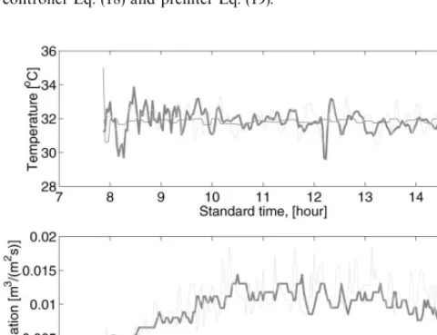
Fig. 8. Setpoint, measured (bold) and predicted (gray) temperatures (top frame), and actual (bold) and simulated desired ventilation rates (bottom frame), for June 14, 1997. The simulated greenhouse was described by Eq. (6) with;"3, and the ventilation NN.
compare the performance of the robust controller with that of a PI controller. The sensitivity of the closed loop to the accuracy of the ventilation model was also tested. Fig. 8 presents the setpoints, measured temperature, and desired ventilation rate recorded in the greenhouse on June 14, 1997. The temperature and ventilation rate predicted by the closed-loop simulation, using the same controller, are shown in the same "gure. It can be seen
that both the predicted and actual temperature and ven-tilation rates are very similar, which validates the con"
g-uration&model (6) and ventilation NN'as a model of the
greenhouse.
Using this simulator, the performance of the robust controller was compared to that of the PI controller
resulting from an internal model control (IMC) design (Rivera et al., 1986), with a bandwidth of 1/200 rad/s:
G
.'(s)" 1
200B !s/A
#1
!s/A
(20)
and, after discretization using the zero-order-hold method, and computingA
with ;"5:
G .'(q)"
!24.12q#21.12
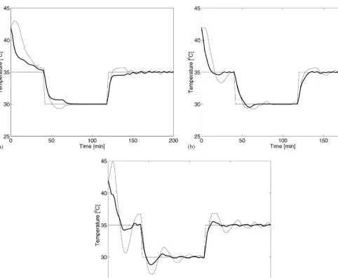
[image:8.596.28.268.298.483.2]q!1 . (21)
Fig. 9 presents the results of the simulations with the robust controller (top left frame), and the PI controller (top right frame), assuming the following constant out-side climate: S
M"500 W/m,¹
M"203C,h M"h
G. It can
be seen that the method used to design the controller, as well as its structure, has only a limited e!ect on the
performance of the loop. The bottom frame of Fig. 9 pres-ents the results obtained with the robust controller if it is assumed that the NN ventilation model is not available to translate the desired ventilation rate into actuator positions. For this simulation, the ventilation rate was translated into actuator positions using the following relations, which, as shown in Fig. 10, are an approxima-tion of the mapping created by the neural network.
ifQ
(0.005,F"2, andO"(Q
/0.005)*50, (22) if 0.005(Q
(0.030, F"(Q
!0.005)/(0.03!0.005)*31, andO"50, (23)
if 0.030(Q
,
F"31, andO"(Q
!0.03)/(0.05!0.03)*50#50.
(24)
A comparison between frames (a) and (c) (robust con-troller with and without NN ventilation model) shows that imperfect modeling of the ventilation rate strongly a!ects the loop performance. A similar deterioration was
observed on the performance of the control loop with the PI controller (not shown).
From these results, it can be concluded that in order to achieve tight temperature control, an accurate relation between the ventilation rate and the actuator positions is required. As long as this relation is available, similar performances can be obtained with di!erent types of
controllers, corresponding to di!erent designs.
6. CO2controller
In order to design the CO
controller, the following
"rst-order model, of which Eq. (2) is a particular case, is
used:
oHdm(t)
Fig. 9. Setpoint and simulated temperatures with the robust controller (Eqs. (18) and (19)) with NN ventilation (frame (a)); PI controller (Eq. (21)) with NN ventilation model (frame (b)); and robust controller (Eqs. (18) and (19)) without NN ventilation model (frame (c)). In each case, the bold line corresponds to;"10 W/mK and the thin one to;"3 W/mK. A constant outside climate is assumed (S
M"500 W/m,¹
M"203C,
q M"q
G).
Fig. 10. Comparison between the desired ventilation rate and the ventilation rate resulting from relations 22}24.
wheremdenotes X G!X
M, * is the delay present in the
control loop, and it has been assumed that the outside CO
concentration is constant.
This model has two uncertain parameters (Qand *), and here again the Horowitz method was chosen to design the controller. The loop delay*, which includes the time to transfer the gas to the sensor and the sensor response time, was determined experimentally to lie be-tween 50 and 110 s. The uncertainty inQwas estimated as $10% of the desired ventilation rate (Q3[0.9;
1.1]Q
). Such a description of the uncertainty allows for the inclusion in the controller of an inverse nominal model (s#Q
/H), where Q3[0.5; 20];10\. At
this point the original system to be controlled can be replaced by
%(s)" 1
oH (s#Q
/H)
[image:9.596.29.260.505.683.2]Fig. 11. COmodel value sets: comparison between the value sets of the original model (Eq. (25)) (upper value set of each frame) and those of the model with cancellation of the nominal plant (Eq. (27)).
Fig. 12. CO
control loop. Nominal open-loop (Eqs. (27) and (28)) and Horowitz bounds at design frequencies.
Fig. 13. CO
control loop. Closed-loop speci"cations (bold), nominal
closed loop (solid line), and gain extent (circles), with the controller described by Eq. (28).
which has the advantage of having its value sets
¢ered' at e\ Q/oH, regardless of Q
. Note that the controlled system now has three uncertain parameters: Q,Q, and*.
This nominal system cancellation can be performed only in continuous time. Therefore, in contrast to the temperature controller, which was designed in the dis-crete-time domain, the CO
controller has to be designed in the continuous-time domain. In a second stage, the controller (containing the inverse nominal model) is translated into the discrete form using the matched pole-zero transformation (Franklin and Powell, 1980). Note that an additional delay of 60 s (t
Q/2) has to be introduced
to model the averaging operation over the two-minute sampling intervals, so that the controller is designed
using the model
%(s)" 1
oH (s#Q
/H)
(s#Q/H) e\ >Q. (27)
The controller is designed to meet the following refer-ence-step speci"cations: maximum overshoot 20%, rise
[image:10.596.289.531.47.246.2]time (80%) 240}600 s, settling time ($10%) 960 s.
Fig. 11 presents typical value sets. In order to show the advantage of introducing the inverse nominal model, the same"gure presents the value sets of the original model
(Eq. (25)). The value sets are clearly reduced by the nominal system cancellation, which allows for the meet-ing of tighter speci"cations, or alternatively, for using
a weaker controller. Fig. 12 presents the Horowitz bounds (the sensitivity bounds were computed with a 6 dB speci"cation), and the nominal open loop with the
controller
G
!-(s)"0.013
1 s
((3s/0.015#1))
(s/(0.015(3)#1)
(1!e\QRQ)
120s . (28)
Here again, this controller was designed by trial-and-error loop shaping such that the nominal open-loop frequency values (denoted by H in Fig. 12) fell on the permissible side of their respective Horowitz bounds.
Note that the last factor in Eq. (28) is the transfer function for the sample-and-hold operation. The dis-crete-domain equivalent of the controller, including the inverse nominal model, is given by
C
!-(q)"0.013
120 (q!1)
(q!e\(RQ) (q!e\RQ()
(q!e\/&RQ) (q!1) .
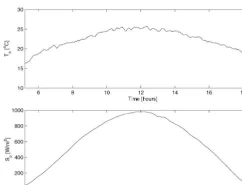
[image:10.596.28.265.310.491.2]Fig. 14. Outside air temperature (top frame), and outside solar radi-ation (bottom frame) recorded on June 4, 1997.
Fig. 15. Implementation results. The top frame presents setpoint (bold) and measured temperature (thin line). The second frame presents the ventilation rate prescribed by the controller. The third frame presents the setpoint (bold) and measured CO
concentration (thin line), and the bottom frame presents the enrichment rate. All"gures present 10-min
averages.
Fig. 13, which presents the frequency-domain speci"
ca-tions together with the nominal closed loop and the gain extent, shows that no pre"lter is required.
7. Implementation results
The controllers described in the previous sections were implemented in the experimental greenhouse. The tem-perature and CO concentration setpoints were com-puted according to the optimization method described by Linker et al. (1998). Fig. 14 presents the outside solar radiation and temperature recorded on June 4, 1997 (the humidity, not shown here, was almost constant at 0.015 kg(vapor)/kg(air)). Fig. 15 presents the computed setpoints, and the control and measured variables for the same day. After a few hours during which no ventilation is applied, and the only ventilation is due to leakage, the air temperature reaches its maximum allowed value (323C in this case). Ventilation is then applied, and it can
be seen that by carefully balancing ventilation and CO enrichment, both the temperature and CO
setpoints can be maintained. Because of the heat storage of the green-house, the optimal operation is not symmetrical around noon. For a given level of solar radiation, maintaining the same temperature in the afternoon requires more ventilation than in the morning. This asymmetry in the ventilation rate is re#ected in the enrichment rate, with
a higher enrichment rate required to maintain the same setpoint. The CO
overshoot at the end of the day is due to the sudden reduction of the ventilation rate, which is responding to the low solar radiation. The enrichment rate is also reduced, but since, as stressed in Section 3, ventilation is not used to lower the CO
concentration, the overshoot remains.
8. Conclusions
The possibility of simultaneously controlling the tem-perature and CO
concentration in a greenhouse has been demonstrated. In particular, it has been shown that, if carefully balanced, ventilation and CO enrichment can be used together, in order to maintain the optimal temperature and a high CO
concentration. Decoupling the temperature and CO
control loops, and using the ventilation rate predicted by the temperature controller as the nominal one when computing the enrichment rate, reduced the CO
model uncertainty, and allowed for tighter control to be achieved.
[image:11.596.26.269.45.230.2]predicted ventilation rate is used in the CO
control loop, inaccurate modeling of the ventilation would also de-grade the performance of this loop. It has also been shown that if such a relationship is available, the method used to design the controller, as well as the type of the resulting controller, has only a limited in#uence on the
loop's performance.
The CO
concentration proved to be more di$cult to
control accurately than the temperature, mainly because of the delay existing in the feedback loop. This delay resulted from the response time of the sensor, which could not be changed, and the time required to transfer the gas to the sensor. The latter could be reduced by placing the sensor closer to the sampling points (its present location is about 20 m from the sampling points). However, in the absence of special cooling arrangements this would expose the sensor to the excessively high greenhouse temperature. The results presented here sug-gest that such costly arrangements are not required. Due to the decoupling between the temperature and CO
control loop, the ventilation is not used to lower the CO
concentration and, as a result, the CO
concentration sometimes presents large overshoots. However, since a high CO
concentration always has a positive e!ect on
crop photosynthesis, using the ventilation to lower the CO
concentration would indeed be wasteful.
Acknowledgements
This study was supported by BARD, Project IS-1995-91RC, by the Israel Ministry of Agriculture, Project 838-0375-92, and by the Technion Fund for the Promotion of Research.
References
AsstroKm, K. J., & Wittenmark, B. (1994).Adaptive control. Englewood
Cli!s, NJ: Addison-Wesley.
Bailey, B. J., & Chalabi, Z. S. (1994). Improving the cost e!ectiveness of
greenhouse climate control.Computers and Electronics in Agricul-ture,10, 203}214.
Barmish, B. R. (1988). New tools for robustness analysis. InProceedings of the 27th IEEE Conference on Decision and Control, Austin, TX (pp. 1}6).
Boaventura Cunha, J., Couto, C., & Ruano, A. E. B. (1997). Real time parameter estimation of dynamic temperature and humidity models for greenhouse adaptive climate control. InPreprints of the 3rd IFAC/ISHS Workshop on Mathematical and Control Applications in Agriculture(pp. 49}54).
Chao, K., & Gates, R. S. (1996). Design of switching control systems for ventilated greenhouses. Transactions of the ASAE, 39(4), 1513}1523.
Chotai, A., Young, P. C., Davis, P., & Chalabi, Z. S. (1991). True digital control of greenhouse systems. In: Proceedings of the First
IFAC/ISHS Workshop on Mathematical and Control Applications in Agriculture and Horticulture. pp. 41}45.
Davis, P. F., & Hooper, A. W. (1991). Improvement of greenhouse heating control.Transactions of IEEE,138(3), 249}255.
Demuth, H., & Beale, M. (1992).Neural network toolbox for use with Matlab. Users guide. MA: Natick.
Franklin, G. F., & Powell, J. D. (1980).Digital control of dynamic systems. Reading. MA: Addison-Wesley Publ.
Gutman, P. O. (1981). Stabilizing controllers for bilinear systems.IEEE Transactions on Automatic Control,26, 917}922.
Gutman, P. O., Levin, H., Neumann, L., Sprecher, T., & Venezia, E. (1988). Robust and adaptive control of a beam de#ector. IEEE Transactions on Automatic Control,33(7), 610}619.
Gutman, P. O., Lindberg, P. O., Ioslovich, I., & Seginer, I. (1993). A non-linear optimal greenhouse control problem solved by linear programming. Journal of Agriculture Engineering Research, 55, 335}351.
Horowitz, I. M., & Sidi, M. (1972). Synthesis of feedback systems with large plant ignorance for prescribed time-domain tolerances. Inter-national Journal of Control,16(2), 287}309.
Idso, K. E., & Idso, S. B. (1994). Plant responses to atmospheric CO enrichment in the face of environmental constraints: A review of the past 10 years'research. Agricultural and Forest Meteorology, 69,
153}203.
Ioslovich, I., Seginer, I., Gutman, P. O., & Borshchevsky, M. (1995). Sub-optimal CO
enrichment of greenhouses.Journal of Agriculture Engineering Research,60, 117}136.
Kimball, B. A. (1986). In#uence of elevated CO
on crop yield. In: B. A. Kimball, & H. Z. Enoch,Carbon Dioxide enrichment of greenhouse crops. Vol. 2:Physiology, yield, and economics. (Chapter 8). Boca Raton, FL: CRC Press.
Linker, R. (1995).Simultaneous CO2enrichment andventilation of green-houses. M.Sc. Thesis. Technion, Haifa, Israel.
Linker, R., Seginer, I., & Gutman, P. O. (1998). Optimal control of CO in a greenhouse modelled with neural networks.Computers and Electronics in Agriculture,19, 289}310.
Nederho!, E. M., van de Vooren, J., & Udink ten Cate, A. J. (1984).
A method to determine ventilation in greenhouses.Acta Horticul-turae,148, 345}358.
Nishina, H., Umakoshi, K., & Hashimoto, Y. (1997). Control of air temperature in nursery plants production system by LQI control with Kalman"lter. InPreprints of the 3rd IFAC/ISHS Workshop on Mathematical and Control Applications in Agriculture(pp. 13}18).
Rivera, D. E., Morari, M., & Skogestad, S. (1986). Internal model control. 4. PID controller design.Industrial and Engineering Chem-istry Process Design and Development,25, 252}265.
Seginer, I., Angel, A., Gal, S., & Kantz, D. (1986). Optimal CO enrichment strategy for greenhouses: a simulation study.Journal of Agriculture Engineering Research,34, 285}304.
Seginer, I., Shina, G., Albright, L. D., & Marsh, L. S. (1991). Optimal temperature set points for greenhouse lettuce.Journal of Agriculture Engineering Research,49, 209}226.
Sigrimis, N., & Rerras, N. (1996). A linear model for greenhouse control. Transactions of the ASAE,39(1), 253}261.
Takakura, T., Manning, T. O., Giacomelli, G. A., & Roberts, W. J. (1994). Feedforward control for a#oor heat greenhouse. Transac-tions of the ASAE,37, 939}945.
Tantau, H.-J. (1991). Optimal control for plant production in green-houses. InProceedings of the 1st IFAC/ISHS Workshop on Mathemat-ical and Control Applications in Agriculture and Horticulture. (pp. 1}6).