Modelling sun-induced fluorescence and photosynthesis with a land surface model at local and regional scales in northern Europe

www.biogeosciences.net/14/1969/2017/ doi:10.5194/bg-14-1969-2017

© Author(s) 2017. CC Attribution 3.0 License.

Modelling sun-induced fluorescence and photosynthesis with a land

surface model at local and regional scales in northern Europe

Tea Thum1, Sönke Zaehle2, Philipp Köhler3, Tuula Aalto1, Mika Aurela4, Luis Guanter3, Pasi Kolari5, Tuomas Laurila4, Annalea Lohila4, Federico Magnani6, Christiaan Van Der Tol7, and Tiina Markkanen1

1_{Climate Research, Finnish Meteorological Institute, P.O. Box 503, 00101 Helsinki, Finland}

2_{Biochemical Integration Department, Max Planck Institute for Biogeochemistry, Hans-Knöll-Str. 10, 07745 Jena, Germany} 3_{Helmholtz-Centre Potsdam, GFZ German Research Centre for Geosciences, Section 1.4 Remote Sensing,}

Telegrafenberg, 14473 Potsdam, Germany

4_{Atmospheric Composition Research, Finnish Meteorological Institute, P.O. Box 503, 00101 Helsinki, Finland} 5_{Department of Physics, University of Helsinki, 00014 University of Helsinki, Finland}

6_{University of Bologna, Via Zamboni, 33, 40126 Bologna, Italy}

7_{Deparment of Water Resources, Faculty ITC, University of Twente, P.O. Box 217, 7500 AE Enschede, the Netherlands}

Correspondence to:Tea Thum (tea.thum@fmi.fi)

Received: 25 November 2016 – Discussion started: 28 November 2016 Revised: 2 March 2017 – Accepted: 9 March 2017 – Published: 11 April 2017

Abstract. Recent satellite observations of sun-induced chlorophyll fluorescence (SIF) are thought to provide a large-scale proxy for gross primary production (GPP), thus pro-viding a new way to assess the performance of land surface models (LSMs). In this study, we assessed how well SIF is able to predict GPP in the Fenno-Scandinavian region and what potential limitations for its application exist. We imple-mented a SIF model into the JSBACH LSM and used active leaf-level chlorophyll fluorescence measurements (Chl F) to evaluate the performance of the SIF module at a conif-erous forest at Hyytiälä, Finland. We also compared simu-lated GPP and SIF at four Finnish micrometeorological flux measurement sites to observed GPP as well as to satellite-observed SIF. Finally, we conducted a regional model simu-lation for the Fenno-Scandinavian region with JSBACH and compared the results to SIF retrievals from the GOME-2 (Global Ozone Monitoring Experiment-2) space-borne spec-trometer and to observation-based regional GPP estimates. Both observations and simulations revealed that SIF can be used to estimate GPP at both site and regional scales. At re-gional scale the model was able to simulate observed SIF averaged over 5 years withr2of 0.86. The GOME-2-based SIF was a better proxy for GPP than the remotely sensed fA-PAR (fraction of absorbed photosynthetic active radiation by vegetation). The observed SIF captured the seasonality of the

photosynthesis at site scale and showed feasibility for use in improving of model seasonality at site and regional scale.

1 Introduction

The terrestrial biosphere is thought to store approximately a quarter of the carbon dioxide (CO2) released by

anthro-pogenic activity (Le Quéré et al., 2016). However, a detailed spatio-temporal distribution of this uptake is absent, partly due to an incomplete understanding of the terrestrial bon balance as a whole. Estimates of the terrestrial net car-bon balance are often made by land surface models (LSMs) (Sitch et al., 2015). However, assessing and improving the performance of LSMs at larger scales remains a challenge, as limited data sources for large-scale carbon dioxide flux esti-mates are available (Luo et al., 2012). Increasing our knowl-edge of carbon dioxide uptake will thus help to provide better estimates of the global carbon balance.

photosynthet-ically active radiation (PAR) is absorbed by the vegetation (Pinty et al., 2011). Recently, global retrievals of sun-induced chlorophyll fluorescence (SIF) have also become available for the monitoring of global vegetation productivity (e.g. Frankenberg et al., 2011; Joiner et al., 2011).

Chlorophyll fluorescence (Chl F) takes place in plant leaves when they photosynthesize. The light energy absorbed by the chlorophyll molecules is used in photosynthesis, dissi-pated as heat or re-emitted as light through ChlF (Maxwell and Johnson, 2000). Thus, Chl F correlates with two si-multaneous processes: photosynthesis and heat dissipation. Therefore, Chl F has been a standard measurement at the leaf scale in plant physiology for decades (Baker, 2008). The advent of retrieval approaches for satellite data acquired by the spectrometers FTS (Fourier transform spectrome-ter; onboard satellite GOSAT), SCIAMACHY (satellite EN-VISAT), GOME-2 (Global Ozone Monitoring Experiment-2; satellite MetOp-A and B) and OCO-2 have demonstrated that it is possible to measure SIF from space (e.g. Frankenberg et al., 2011, 2014; Guanter et al., 2012, Joiner et al., 2012, 2013; Köhler et al. 2015).

As the seasonal cycles of fAPAR and SIF are related to radiation and greenness of the vegetation, they appear sim-ilar in many ecosystems. However, SIF is more physiologi-cally related to photosynthesis and has been shown to track gross primary production (GPP) better than fAPAR in de-ciduous broadleaf and mixed forests as well as in croplands (Joiner et al., 2014). Moreover, comparison to observation-based upscaled global GPP products (Jung et al., 2011) has suggested that SIF is a better estimator of GPP than other traditional remotely sensed vegetation indices, such as EVI (enhanced vegetation index) and NDVI (Frankenberg et al., 2011; Walther et al., 2016), and may thus be of relevance in the observation or modelling of the terrestrial carbon balance (Lee et al., 2015; Parazoo et al., 2013).

SIF can be estimated from state-of-the-art photosynthesis models, such as the widely used Farquhar model (Farquhar et al., 1980), by describing the processes of photosynthesis and fluorescence at the cellular level (van der Tol et al., 2009a) or leaf level (van der Tol et al., 2014). The strong dependence of the measurable SIF signal on scattering and reabsorption ef-fects within the canopy requires explicit formulation of the radiative transfer (e.g. SCOPE; van der Tol et al. 2009b). Nevertheless, modelling studies using satellite-observed SIF have revealed links between forest productivity and water stress in the Amazon (Lee et al., 2013) and have helped to constrain the seasonal cycle of GPP (Parazoo et al., 2014). Koffi et al. (2015) included SIF in their global carbon cycle data assimilation system and found SIF to be more sensitive to the chlorophyll content in the leaves than to the parameter maximum carboxylation rate controlling model GPP.

The challenge in using the space-borne SIF data for the evaluation of SIF models is the lack of similar ground-based observations, and the degree of correspondence be-tween GPP and SIF at different spatial scales. Another

im-portant consideration is that the SIF observation from space is dependent on a passive measurement carried out in nar-row spectral bands. The signal in the red region originates mostly from the top of the canopy, whereas deeper canopy layers also contribute to the far-red signal (Porcar-Castell et al., 2014). Both these regions can be used in retrieving SIF from remote sensing observations.

Our aim in this study is to assess whether the SIF mea-surements can be used to quantify the LSM performance at a regional scale for the spring and autumn transition periods. Forests in the boreal zone experience a strong seasonal cycle with cold winters and warm summers (Bonan, 2008). The transition periods of spring and autumn influence the carbon balances in these northern ecosystems (Bergh et al., 1998). In a changing climate the conditions in spring and autumn will change (Ruosteenoja et al., 2011) and cause changes to car-bon balances. It is anyhow during these times that the carcar-bon cycle models have difficulties in performance (Schaefer et al., 2012). Therefore, it is important to find ways to improve carbon cycle models in these time periods.

In Fenno-Scandinavia coniferous forests are very common and study of their photosynthetically active period with re-mote sensing products is a challenge because of the stronger relative contribution to the GPP cycle of the physiologi-cal seasonal cycle than the changes in green foliage area (Böttcher et al., 2014). Our strategy consists of implementing a ChlF model into the LSM JSBACH model and evaluat-ing the results of this implementation. We examined the per-formance of the model by comparing it to leaf-level ChlF

observations at the site scale in one forest. We then evalu-ated the model performance at four coniferous forest sites by comparing the remotely sensed SIF signal from GOME-2, modelled SIF and the modelled GPP to observations with the eddy covariance technique. Finally, we made a regional model run for Fenno-Scandinavia and compared our results to satellite observations.

2 Materials and methods

2.1 Active and passive measurements of ChlF in general

Active measurements of ChlF in field conditions are typi-cally done with the pulse amplitude modulated (PAM) tech-nique where ChlF is measured over a broad spectral region (Porcar-Castell et al., 2014). In the active measurement, a weak and pulsed measuring light is used to excite fluores-cence. The Chl F measured by the PAM technique is not dependent on the prevailing light environment, but reflects the efficiency in transforming the measuring light into fluo-rescence. The active measurement provides the fluorescence signalF0and the photosynthesis yield8p, which describes

(i.e. heat dissipation) and8p, it is also necessary to have ob-servations of adapted leaf, as it is assumed that dark-adapted leaf with all the reaction centres open do not exhibit NPQ (Murchie and Lawson, 2013).

Passive measurements are an alternative to active observa-tion of ChlFand rely on the emission under natural light en-vironments, where the SIF is estimated in very narrow spec-tral bands and is affected by ambient illumination (Porcar-Castell et al., 2014). Passive measurements can be ground-based, but also based on remote sensing carried out on the ground or from space (Meroni et al., 2009). Passive observa-tions rely on the in-filling of atmospheric or solar absorption lines by SIF. The ChlF yield (8f)can be obtained from the passive measurements and it is an indication of the fraction of electrons in the leaf follow the ChlF pathway.

Thus, passive measurements provide SIF and fluorescence yield 8f values, whereas the active measurements provide the prevailing fluorescence signalF0 and yield of photosyn-thesis8p. In non-stressed low-light conditions, most of the

absorbed energy is used for photosynthesis (causing higher

8p)that results in lower fluorescence yield (8f). Therefore,

an inverted relationship exists between ChlF and photosyn-thesis yields at low-light levels (van der Tol et al., 2009a). However, during high-light and/or stressed conditions NPQ is increased and then8pand8fare positively correlated.

2.2 Models 2.2.1 JSBACH

We used the biosphere model JSBACH (Reick et al., 2013) that is part of the Max Planck Institute’s Earth System Model (Giorgetta et al., 2013). In addition to the global simulations, JSBACH can also be applied at regional and site scales.

The JSBACH model simulates the exchanges of carbon, water and energy between the land surface and the atmo-sphere. The incoming radiation that reaches the canopy is calculated for the three different canopy layers using a two-stream approximation model (Dickinson, 1983; Sellers, 1985). In this model, it is assumed that the distribution of scattering objects in the canopy is homogenous so that the radiation distribution inside the canopy is horizontally in-variant. Therefore, it is necessary to only consider vertical radiant fluxes.

fAPAR for one layer is calculated as fAPAR(lnln+1)=

Itot(ln)−Itot(ln+1) Rdir(0)+Rdiff(0)

, (1)

where ln is the cumulative leaf area index (LAI) for the canopy layer,Itotis the total incoming radiation that reaches

the canopy layer and includes the direct incoming radiation to the canopy layer and upward and downward diffuse radi-ation.Rdir(0) is the direct radiation at the top of the canopy,

andRdiff(0) is the incoming diffuse radiation at the top of the canopy. The absorbed radiation for each canopy layer is

used in the photosynthesis calculation. The fAPAR for the whole canopy is obtained by summing the values from the three different layers together.

In this model, photosynthesis is described by the Farquhar et al. (1980) formulation for C3 plants and stomatal conduc-tance is based on Knorr (2000) (photosynthesis for C4 plants follows Collatz et al. (1992), but these species are not rel-evant in our study region). Photosynthesis is either electron transport rate or maximum carboxylation rate limited. The electron transport rateJ from the photosynthesis model is used in the calculation of chlorophyll fluorescence and its formulation is as follows:

J (I )=Jmax

αI p

J2

max+α2I2

, (2)

where Jmax is the maximum electron transport rate (unit:

µmol m−2s−1) with a linear air temperature dependency,

I is incoming photosynthetically active radiation (unit: µmol m−2s−1) and α is the apparent quantum yield (value 0.28).

The vegetation in JSBACH is described by plant func-tional types (PFTs). Different PFTs have specific physiolog-ical properties such as photosynthetic capacity and physphysiolog-ical properties, e.g. the albedo of the canopy. Each grid cell can contain up to four different PFTs and we used 13 potentially different PFTs for vegetation in our simulation. The vegeta-tion map was based on the European Corine Database, de-scribed in Törmä et al. (2015). The leaf area development in JSBACH is based on the LoGro-P (Logistic Growth Phe-nology) model (Böttcher et al., 2016). Air temperature is the main driver of the phenological development in the two main vegetation types (evergreen needleleaf forests and temperate deciduous broadleaf forests) in our study region.

2.2.2 Leaf-level chlorophyll fluorescence

The model equations for the leaf-level fluorescence are shown in Appendix A. The outputs of the model are SIF and scaled fluorescence yield8f,s. Due to simplifying

assump-tions, such as lack of wavelength separation, we do not sim-ulate the magnitude of SIF with JSBACH. However, seasonal changes in the modelled SIF are still captured. In the ChlF -related literature, the ChlF quantities are often referred to as parameters, but in this work the word parameter will refer to a model parameter that is kept constant and ChlF-related observations are instead referred to as variables.

2.2.3 Canopy scaling

In order to derive a comparatively simple, computationally efficient scheme for the emission and extinction of radiation in the fluorescence wavelengths, we developed a simplified parameterization with the form

SIFcan= nlayers

X

i=1

SIFi×e

(−kfl_nLAItot

where SIFcanrefers to the SIF signal that originates from the

whole canopy,nlayers is the number of canopy layers in JS-BACH,kflis the attenuation coefficient and LAItotis the total

LAI of the canopy. This equation is based on the output of the comprehensive radiative transfer model SCOPE and de-scribes the radiative transfer, photosynthesis, chlorophyll flu-orescence, temperature and energy balance at site-level for a given canopy structure (van der Tol et al., 2009b).

We used the SCOPE model version 1.52b in our study. We derived the parameterization of Eq. (3) by first calculating the hemispherically integrated top of the canopy value for SIF when emission was coming from only one canopy layer at a time. Thus, we obtained a profile of how much of the emission that originated from each canopy layer reached the top of the canopy. Dividing this profile by the emission of the different layers yielded the attenuation of the ChlF sig-nal in the canopy. The derived attenuation coefficientkflwas slightly sensitive to the wavelength considered, while chang-ing the amount of foliar mass/area did not affect the atten-uation coefficient. The attenatten-uation coefficientkfl also varied

with the solar hourly angle;kfl for wavelength 740 nm was

0.350 at noon and 0.347 at 10.30 am, which corresponds to the approximate local solar time of the GOME-2 observation. Therefore, we used the attenuation coefficientkflvalue 0.347

in our analysis.

2.3 Measurements

2.3.1 Site-level ChlF and carbon dioxide (CO2)flux measurements at Hyytiälä

The Chl F site-level measurements are from a Scots pine (Pinus sylvestris) forest at Hyytiälä, Finland (61◦510N, 24◦170E; 180 m a.s.l.) (Kolari et al., 2009). The forest was planted in 1962 after burning and mechanical soil prepara-tion. The soil is a Haplic Podzol on glacial till and the site is of medium fertility (Kolari et al., 2009). The forest also has a sparse understory of Norway spruce (Picea abies). The total LAI is 6 m2m−2for the Scots pine. The CO2flux

be-tween the vegetation and the atmosphere was measured con-tinuously with a closed-path eddy covariance system that is described in more detail in Rannik et al. (2004) and Mam-marella et al. (2009). Gap-filling and flux partitioning are de-scribed in Kolari et al. (2009).

Chl F was measured in the Scots pine needles with a MONITORING-PAM Multi-Channel Chlorophyll Fluo-rometer (Walz, Effeltrich, Germany) (Porcar-Castell et al., 2008; Porcar-Castell, 2011). The measurement period was 15 August 2008–14 August 2009. The measurement sys-tem MONITORING-PAM uses a modulated blue LED light to measure the fluorescence emitted from the leaf sample (Porcar-Castell, 2011). We used the results from an emitter-detector unit that measured three or four pairs of needles ar-ranged in a leaf clip. The unit was located in the mid-canopy.

The instrument recorded instantaneous fluorescence (F0), maximal fluorescence (F m0) and incident PAR radiation. During nighttime, the maximal fluorescence (F m) and the minimal fluorescence (F o) were measured. The observations were done every 10 min during summer and every 30 min during winter. The temperature sensitivity of the LED mea-suring light was corrected in the absolute fluorescence levels (Porcar-Castell, 2011). From the measured ChlF variables it was possible to calculate the quantum yield of photosystem II (PSII) by8p=(F m0−F0)/F m0.

2.3.2 Other CO2flux measurement sites

In addition to Hyytiälä (FI-Hyy), we used measurements from three other Finnish flux measurement sites. Together these four sites cover a wide latitudinal range, with the two southern sites: Hyytiälä and Kalevansuo (FI-Kns) located in the southern boreal zone. Two sites are located north of the Arctic Circle: Sodankylä (FI-Sod) and Kenttärova (FI-Ken) in the northern boreal zone. FI-Ken is a Norway spruce for-est, whereas the other sites are Scots pine forests. More site information can be found in Table 1.

2.3.3 Observations from space, SIF and fAPAR To obtain estimates for SIF, we used data from GOME-2 (Global Ozone Monitoring Instrument 2), which is an op-erational medium resolution nadir-viewing ultraviolet (UV)– visible and near-infrared cross-track scanning spectrometer onboard EUMETSAT’s polar orbiting MetOp-A and B (Me-teorological Operational Satellites) (Munro et al., 2006). The spectrometer measures the Earth’s backscattered radiance and the extraterrestrial solar irradiance. The overpass time of the satellite is around 09:00 LST (local solar time) at the Equator, while one revolution takes 100 min. Here, we use the GOME-2 SIF data set derived with the approach pre-sented by Köhler et al. (2015). The retrieved SIF data were available for 2007–2011, with an 8-day time resolution and a spatial resolution of 0.5◦×0.5◦. Typical SIF error estimates range up to 0.5 mW m−2sr−1nm−1(Köhler et al., 2015).

In our analysis, we also used the space-observed variable fAPAR. These values were obtained by partitioning the solar radiation fluxes that were based on inversion of the MODIS broadband white sky surface albedos (Pinty et al., 2011). Temporal resolution was 16-days and spatial resolution 1 km. Monthly values of fAPAR were used in the analysis. 2.4 Simulations

2.4.1 Site-level simulations

Table 1.Measurement sites.

Abbreviation Name Location Vegetation Total LAI Year Reference (m2m−2)

FI-Kns Kalevansuo 60◦390N, Scots pine 5 2007–2008 Lohila et al. (2011) 24◦210E forest

FI-Hyy Hyytiälä 61◦510N, Scots pine 6 2007–2011 Rannik et al. (2004)

24◦180E forest Mammarella et al. (2009)

FI-Ken Kenttärova 67◦590N, Norway spruce 6.6 2007–2011 Thum et al. (2008)

24◦150E forest Aurela et al. (2016)

FI-Sod Sodankylä 67◦210N, Scots pine 3.6 2007–2008 Thum et al. (2007) 26◦380E forest

et al., 2011) were used to fill the missing values in the me-teorological time series. The seasonal maximum of LAI of the model over several years was matched to the observed value. The maximum carboxylation rate Vc(max) and maxi-mum potential electron transport rateJmaxparameters were adjusted so that the modelled GPP matched the magnitude of the observation-based GPP. The two parameters have a fixed ratio andJmaxwas fixed accordingly. No rigorous parameter inversion methods were used, as we did not use the absolute GPP values in our study, but focused more on the seasonal behaviour. In JSBACH, these two Farquhar model parame-ters have a vertical profile, which were here assumed to cor-respond to the observed vertical distribution of foliar nitro-gen content (in units leaf mass per area) at FI-Hyy (Palmroth and Hari, 2001).

A comparison of leaf-scale observations with the PAM technique to site-scale simulated values is somewhat diffi-cult, as the PAM measurement provides the photosynthesis yield 8pand fluorescence signal F0, whereas JSBACH

in-cludes the “passive” fluorescence yield8fand when multi-plied by the radiation provides an estimate of SIF. Notwith-standing these differences, the seasonal cycle of both values may be compared in relative terms as both are connected to the activity of the photosynthetic apparatus in the plants. The observed GPP is obtained from the flux tower and is, there-fore, at the same scale as the simulation output.

At four micrometeorological measurement sites, the mod-elled SIF and GPP were compared to observed GPP and satellite observations of SIF. Averages of the 2◦×2◦spatial resolution pixels closest to the flux tower from the satellite observations were used with a 20-day time period. Averages were used rather than the closest pixel to the site, as spa-tial averaging reduces the retrieval data error. At the north-ern sites, some satellite observations from mid-winter were absent due to cloud contamination. Therefore, those time pe-riods were omitted from the analysis. In addition, the time period 09:00–11:00 LST was taken from the model results and flux measurements to allow for comparability with the satellite observations.

2.4.2 Regional-scale simulations

The modelling domain consisted of Fenno-Scandinavia (52– 74◦N, 4–44◦E). The meteorological data for JSBACH were prepared with the regional climate model REMO (Jacob and Podzun, 1997; Jacob, 2001; Jacob et al., 2001), which was run with an hourly time step driven by the six hourly bound-ary conditions obtained from the ERA-Interim re-analysis (Dee et al., 2011). The resolution of REMO in our set-up is 0.1667◦_{. The JSBACH regional run had the same spatial and}

temporal resolutions. In this study, we focused on the region 52–72◦N, 4–32◦E.

We made comparisons between modelled and observed SIF and also between modelled SIF and GPP and the MPI-BGC GPP product that is available at monthly timescales (Jung et al., 2009, 2011). The GPP product is data based and has been upscaled for regional and global scales using the model tree ensemble approach. For the analysis the model grid points with less than 50 % of vegetation cover were omitted.

3 Results

3.1 Annual time series of ChlF and GPP at leaf and site scale

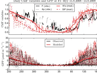
Observed ChlF and GPP had a pronounced annual cycle at Hyytiälä forest (Fig. 1). The observed quantum yield of pho-tosynthesis8pdecreased to a low winter level later than the observed fluorescence signalF0. TheF0started to decrease around day-of-year (doy) 280, later than the observed GPP flux, which was reduced to zero around mid-November. The increase in observed ChlF variables:F0and8p, took place at the same time in spring and this was also connected to the beginning of photosynthesis.

Simulated SIF decreased earlier in autumn than the other Chl F variables. This was likely associated with the de-cline in incoming radiation. The simulated GPP was a good match with observations during autumn. The simulated8f,s

m m

Figure 1. (a)The annual cycles (15 August 2008–14 August 2009) of measured chlorophyll fluorescence (F0and photochemical yield8p)

and the simulated ChlFvariables (SIF and fluorescence yield8f,s)from the JSBACH model at a daily scale at site FI-Hyy. All the ChlF

variables are scaled from 0 to 1. The thick line for the modelled ChlFvalues is a 15-day running average of the value.(b)The modelled and observed gross primary production (GPP) at half-hourly means (dots) and corresponding 30-day running mean (thick lines).

a lower level compared to them. This might be connected to the way electron transport rate (ETR) was simulated in the model. In the Farquhar model the temperature dependency of the parameter has much of influence on ETR, whereas the observed ChlFvariables gave reason to suggest that the ETR stayed on a higher level later to the winter. The gradual de-cline of the observed ChlF variables might be due to dark autumns, as the needles do not suffer from excess light levels and thus the downregulation of the light harvesting machin-ery can be much lower (Kolari et al., 2014). The yield of photochemistry and fluorescence declines during winter be-cause the yield of NPQ increased in a process regulated by air temperature (Porcar-Castell, 2011).

The observed ChlF variables drop to their lowest value in February and March. This was the time period when the forest was experiencing stress because of the increasing light levels, but still persisting soil freeze and low air temperatures. The trees will have need for photoprotection in order to get rid of the excess light energy that they cannot yet use for pho-tosynthesis, because of the prevailing conditions. Therefore, the observed ChlF values obtained their lowest values in this time period. The low values in the simulated ChlF variables are only caused by low temperatures; the mechanisms related to photoprotection are not included in the current model im-plementation.

Simulated 8f,s showed an earlier ascent in spring, and

this was connected to simulated photosynthesis that com-menced too early, clearly seen in the half-hourly GPP values in Fig. 1b. The comparison between simulated8f,s, SIF and

observed incoming PAR showed that in spring8f,s slowed

down the increase of SIF to its summertime values, whereas in autumn light limitation caused the withdrawal of SIF (Sup-plement, Fig. S1).

Some negative GPP values are present in Fig. 1. The ran-dom nature of turbulence and instrument uncertainty adds to measurement uncertainty (Rannik et al., 2016). The GPP is obtained from the observed net ecosystem exchange by sub-tracting the respiration that has been estimated by a regres-sion fit to temperature (Wohlfahrt and Galvano, 2017). Thus, the random measurement error leads to some negative GPP values that are compensated by an equal amount of too high positive values; additionally, the temperature fit to respiration causes some systematic error in the values.

ObservedF0 and8p decreased at high light levels on a

sunny day (Fig. S2). While this decline also occurred in sim-ulated8f,s, simulated SIF is increased with incoming

radia-tion. On a cloudy day, observedF0increased during the day, whereas8pshowed some decrease from the morning value (Fig. S3). Simulated8f,sand SIF both increased during

Figure 2.The daily cycle of simulated SIF and8f,sin three different canopy layers of JSBACH on day 160 in 2008. Layer 1 was the upmost

layer without attenuation taken into account in(a)and(b)and with attenuation estimated from the SCOPE model included in(e)and(f). The sums of different layers are shown in(c)(SIF) and(d)(8f,s)with and without attenuation.

and8punder low light conditions and the positively corre-lated relationship under high light conditions.

3.2 Upscaling to site scale

In JSBACH, most of the ChlFsignal originated from the top of the canopy, as it received most of the light and, therefore, the largest part of photosynthesis takes place here (Fig. 2). On a sunny day around midday, 86 % of total canopy GPP and 88 % of SIF was produced in the uppermost layer. On a cloudy day 97 % of the total canopy GPP and 98 % of the total canopy SIF was generated in the uppermost layer. 3.3 Comparison of remote sensing results at site scale Overall, the remotely sensed SIF signal followed the seasonal cycle of observed GPP and modelled SIF and GPP at the flux sites (Fig. 3). Observed and modelled SIF showed a larger correlation to observed and modelled GPP, respectively, than fAPAR, in particular the FI-Hyy and FI-Ken sites (Table 2). The model was better at predicting the observed GPP than observed SIF (Table 2), which might reflect the scale mis-match of the SIF observations. Nevertheless, the ability of JSBACH to simulate fAPAR was not as good as its simula-tion of the SIF signal (Table 2).

The modelled GPP had the tendency to increase too early in spring, which was clearly seen at FI-Kns (Fig. 3a) and

FI-Sod (Fig. 3e). This increase happened shortly before the start of the observed photosynthesis. This early emergence of photosynthesis contributed to the inability to simulate the observed SIF signal.

The slope between modelled GPP and SIF was 8.7 g C m−2_d−1_{/(unitless) (standard deviation 0.5 g}

C m−2_d−1_{/unitless) averaged over the four sites}

D

D

Figure 3.Observed and simulated SIF and GPP scaled to unity (unitless) with corresponding standard deviations at(a)FI-Kns,(c)FI-Hyd, (e)FI-Sod,(g)FI-Ken.

Table 2.The correlation coefficient (r2) and its significance (in parenthesis) between modelled and observed sun-induced fluorescence (SIF) (observed SIF in units mW m−2sr−1nm−1) and gross primary production (GPP) (unit: g C m−2d−1) values at different sites. In the calculation of linear regressions between simulated and observed GPP and SIF, 20-day time periods and the morning values were used. In the calculation of GPP vs. fraction of absorbed photosynthetic active radiation by the vegetation (fAPAR) fits, monthly values including the whole day were used.

FI-Kns FI-Hyy FI-Sod FI-Ken

Obs. GPP vs. obs. SIF 0.91 0.93 0.89 0.82

(3.66×10−19) (4.24×10−51) (3.44×10−11) (7.33×10−22)

Mod. GPP vs. mod. SIF 0.99 0.92 0.99 0.83

(1.20×10−34) (5.80×10−85) (1.04×10−29) (1.38×10−29)

Obs. GPP vs. mod. GPP 0.97 0.98 0.84 0.82

(1.25×10−27) (8.02×10−73) (2.06×10−12) (2.40×10−29)

Obs. SIF vs. mod. SIF 0.90 0.90 0.66 0.81

(4.00×10−18) (3.03×10−44) (3.41×10−18) (9.17×10−28)

Obs. GPP vs. obs. fAPAR 0.90 0.66 0.82 0.72

(5.64×10−10) (1.68×10−12) (6.16×10−8) (1.01×10−13)

Mod. GPP vs. mod. fAPAR 0.89 0.86 0.80 0.67

(3.01×10−12) (4.98×10−27) (2.33×10−9) (5.82×10−16)

Obs. fAPAR vs. mod. fAPAR 0.77 0.70 0.72 0.67

(1.58×10−8) (8.26×10−17) 7 (1.53×10−7) (1.31×10−15)

sites, although the fAPAR values showed a similar range at all the sites.

Year 2009 at FI-Ken

Table 3.The slopes of the fits between gross primary production (GPP) and sun-induced chlorophyll fluorescence (SIF)/fraction of absorbed photosynthetic active radiation by vegetation (fAPAR). Note that a constant scalar was used in multiplying the modelled SIF values.

FI-Kns FI-Hyy FI-Sod FI-Ken Average SD

Obs. GPP vs. obs. SIF 7.6 (±0.4) 9.8 (±0.3) 9.5 (±0.7) 7.8 (±0.5) 8.7 1.0 Mod. GPP vs. mod. SIF 8.3 (±0.1) 9.7 (±0.1) 8.5 (±0.1) 9.2 (±0.5) 8.9 0.5 Obs. GPP vs. obs. fAPAR 22.9 (±2.5) 24.1 (±2.5) 13.2 (±1.5) 12.5 (±1.2) 18.2 5.3 Mod. GPP vs. mod. fAPAR 15.8 (±1.2) 18.1 (±0.9) 5.8 (±0.6) 4.3 (±0.4) 11.0 6.0

SPRING

(a)

GOME-SIF

(b)

JSBACH-SIF

(c)

JSBACH-GPP

(d)MPI-GPP

0.0 0.5 1.0

SUMMER

(e) (f) (g) (h)

0.0 0.5 1.0

AUTUMN

(i) (j) (k) (l)

0.0 0.5 1.0

WINTER

(m) (n) (o) (p)

0.0 0.5 1.0

Figure 4.Maps for our study region with GOME-SIF, JSBACH-SIF, JSBACH-GPP and MPI BGC-GPP averaged for time period 2007–2011 and separated between seasons.

(Fig. 3g). In contrast to the observations, the model predicted a drought-related decline in summertime GPP in 2009. This might be due to the presence of a thin humus layer at FI-Ken, which probably makes the site more resistant to drought (Hil-lel, 1980), whereas JSBACH is only able to simulate freely draining upland soils.

The ensuing decoupling of modelled SIF and GPP vari-ables was connected to the current formulation of the actual electron transport rate (Ja)in the model (Eq. A6). The for-mulation of Eq. (A6) states that the actual electron transport rate isJ from Eq. (2) when photosynthesis is limited by the electron transport rate.

At FI-Ken the simulated summer drought influenced the simulated GPP via soil moisture limitation in the stomatal conductance. In the JSBACH model, soil moisture limita-tion causes a reduclimita-tion in both the electron transport and the carboxylation rate-limited branches of photosynthesis. This is different from other models, such as SCOPE, in which drought causes an additional decrease inVc(max)that further drives down the carboxylation rate-limited carbon assimila-tion Ac and results in a shift to carboxylation rate-limited photosynthesis. Closer examination of the FI-Ken simulation results revealed that it was mostly dominated by the electron transport rate-limited photosynthesis; therefore, the drought effect seen in simulated GPP did not lower SIF.

3.4 Regional runs

The correlation between observed and simulated SIF for the averaged 5-year period was reasonably high (r2=0.86) for different grid points in the study region. The correlation be-tween simulated GPP values and the MPI-BGC GPP product was at a similar level (r2=0.78). Overall, simulated GPP values were lower than the estimates from the data-driven MPI-BGC GPP, with the highest simulated GPP values less than 1200 g C m−2yr−1, while most of the grid points lo-cated south of 58◦N according to the MPI-BGC GPP have larger values. The distribution of GPP on the map showed that the MPI-BGC GPP product predicts much larger GPP values for the Norwegian coast than JSBACH (Fig. 4). Dur-ing winter months, larger GPP values than in the surround-ing regions were also seen in the MPI-BGC product (Fig. 4p). The low values in that region in JSBACH originated from the vegetation maps used for the generation of the PFT distribu-tion. A pronounced difference between the model results and observations is that the simulated GPP reached the zero level, whereas this did not occur for the MPI-BGC GPP product, which was not below 380 g C m−2_yr−1_{in our study region.}

o

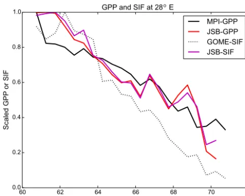
Figure 5. Latitudinal transect at 28◦E showing JSBACH-GPP, MPI-BGC-GPP and observed and simulated SIF averaged for the time period 2007–2008. All quantities have been scaled to unity.

estimates from JSBACH dropped noticeably compared to the MPI-BGC GPP product.

During spring, satellite-observed SIF showed a number of larger values in central Finland (Fig. 4a) that were not seen in the model variables (Fig. 4b–d). In summer, satellite-observed SIF showed a larger gradient in the north–south direction than the model variables (Fig. 4e–h). This might reflect the fact that the observed gradient in green biomass was larger than that seen in the simulations (Markkanen et al., 2017). In autumn, the geographical distribution was quite similar between observed and modelled SIF and GPP vari-ables (Fig. 4i–l). This might be connected to the strong light dependence of SIF and GPP, both in real world and simula-tions, as light is a very important driver for photosynthesis in autumn. At winter, satellite-observed SIF showed some scat-tering in the area where it had values (Fig. 4m). These values were likely connected to the challenges of winter time mea-surements (e.g. low light levels) with GOME-2.

At the seasonal scale, the strongest correlation (r2=0.87) between satellite-observed and simulated SIF occurred in au-tumn (September–November) (Fig. 6c). The high correlation during autumn is likely related to the inherent light depen-dency of both GPP and SIF as light diminishes along lat-itudinal gradient. The slope of the fit between observed and modelled SIF values changed in spring compared to the sum-mer and autumn periods. This was caused by our large latitu-dinal gradient of the region. In the southernmost region there appears to be some linear dependency between modelled and observed SIF, but in the northernmost region the modelled SIF values are still very close to zero.

The seasonal cycle at a monthly resolution for the differ-ent latitudinal regions revealed differences between the mod-elled and observed SIF (Fig. 7a). The highest SIF in the

sim-Figure 6.Correlation plots for different seasons, GOME-SIF vs. JSBACH-SIF. Note that JSBACH-SIF has been multiplied by 100.

ulations occurred in July in all latitudinal regions. However, the highest value in the observations in low-latitude regions occurred in June, whereas in region 62–66◦N highest value took place in July and north of 66◦N the highest value oc-curred in August. Two of the studied micrometeorological measurement sites were located in the northernmost latitu-dinal region. At FI-Ken, observed SIF predicted the highest activity 1 month later than the observed GPP. As with simu-lated SIF, simusimu-lated GPP from JSBACH showed the highest value in July, even though in the two most southern regions June and July were at a similar level (Fig. 7b). The highest values of GPP in Denmark occur in June due to the cultured crops (Lansø, 2016) and similar crops might also influence seasonal cycle in the Baltic region. The GPP from MPI-BGC was similar to the satellite-observed SIF highest value in the southernmost region in June and for the other regions the highest values occurred in July (Fig. 7b).

4 Discussion

4.1 Site-level observations

The implementation of the SIF leaf-scale model into JS-BACH performed appropriately when compared to observa-tions from FI-Hyy, a typical coniferous site for southern Fin-land. The fact that both simulated GPP and ChlF increased earlier than their observed counterparts in spring would sug-gest that ChlF observations might be successful in improv-ing modellimprov-ing of photosynthesis, e.g. in a data assimilation set-up (Koffi et al., 2014; Norton et al., 2017); however, it should also be noted, that the data for FI-Hyy was de-rived from active measurements, and that the coupling be-tween8pand8fmight be changed during different seasons

differ-Figure 7.Averaged seasonal cycles of observed and simulated SIF (a)and MPI-BGC and simulated GPP(b)separated by latitudinal regions. Note that the simulated SIF value was multiplied by 100. The observed SIF is in units mW m−2sr−1nm−1.

ent variables than the “passive” quantities obtained from the model, and therefore there is reason to be cautious with the comparison.

The SIF and fAPAR are close to each other in observa-tions, as they are both related to green biomass. However, in the JSBACH model their calculation is different with fAPAR derived as a function of LAI and radiation, whereas GPP (and therefore SIF) is a function of other environmental variables and model parameters (in addition to LAI and radiation) that may also have an effect.

The photosynthesis of forests is often modelled using con-stant temperature response for the biochemical model param-eters VmaxandJmaxthroughout the year. However, studies

have revealed that this assumption does not hold for ecosys-tems with strong seasonal cycles, but causes overestimation of CO2fluxes in transition periods, at least in spring. Kolari

et al. (2014) found seasonally varying values for leaf level for those parameters from leaf-level observations at FI-Hyy. Ueyama et al. (2016) found seasonally varying biochemical model values at four different black spruce forests in Alaska in a model inversion study at eddy covariance sites. In an ear-lier study using inversion at boreal coniferous forests (Thum et al., 2008), it was found that three forests at northern boreal zone (FI-Hyy, FI-Sod and FI-Ken) had temporal evolution in the biochemical parameters, but a site located on temperate boreal (Norunda, Sweden) did not.

Leaf-level studies have used temperature acclimation for the changes of biochemical parameters (Wang et al., 1996). Similar results have been obtained for site-level results at FI-Sod, where dark-acclimated chlorophyll fluorescence obser-vations have been used in combination with eddy covariance

observations to disentangle the effect of changing maximum photosynthetic capacity (Thum et al., 2017).

The changes taking place in the needles of conifer forests in winter are numerous to protect the needles in challeng-ing environmental conditions. For example, the light harvest-ing complexes are aggregated (Porcar-Castell, 2011) and the xanthophyll cycle enables photoprotection (Ensminger et al., 2004). Some of these processes can in future be included in a large-scale model, as in adding changes to the parameters in the ChlF model discussed below, but, as changes in the boreal spring happen at quite a fast pace and those can be tracked with several different environmental and biological variables (Thum et al., 2009), for large-scale applications a temperature-related changing of the biochemical parameters might be the next step forward and remotely sensed SIF ob-servations provide a very useful evaluation tool in this con-text.

The number of active PSII reaction centres (parameterqLs

in the chlorophyll fluorescence model) has been shown to change seasonally in boreal environments (Porcar-Castell, 2011). However, in our implementation we assumed it to be a constant 0.5, as there is no theory to predict variations of this parameter at larger scales. Similarly, the rate constant of sustained thermal dissipation (parameterkNPQsin the

chloro-phyll fluorescence model) incorporates seasonal variation in boreal forests (Porcar-Castell, 2011), but for the same rea-sons it was kept as zero in our model runs. The comparison with the data nevertheless suggests that these assumptions are justified at the time- and spatial scales of our analysis.

However, since the seasonal cycle was captured quite well by the model at FI-Hyy, even though the seasonally variable parameters that control yield were not considered, some con-cerns connected with the model are evident. The link to the Farquhar model causes the simulated ChlF variables to have a pronounced seasonal cycle similar to the measurements, even though the light reactions of the SIF model does not include the seasonal changes that take place in the leaves. While this could be considered as a counterargument against our approach, the fact that we can generate an appropriate time series with the environmental controls of the Farquhar model suggests that our approach maybe a sensible choice when attempting to simulate SIF at ecosystem and larger scales.

4.2 Satellite data

Here we compared site-level observations with satellite observations, despite the fact that these two observations are at completely different spatial scales. A flux tower measures approximately 1 km2 of the surrounding area, whereas the satellite observations have a wider footprint (e.g. for GOME-2 default footprint is 80 km×40 km). However, Finnish terri-tory consists of large areas of forest and the seasonal cycle is driven by meteorological variations that have an influence at larger spatial scales, and therefore we consider the compari-son between these different scales to be appropriate assuming a homogeneous landscape.

At large scale the ability of SIF to estimate the seasonal cycle of GPP has been shown at boreal coniferous forests (Walther et al., 2016). At the leaf scale the connection is more complex. The seasonal dynamics of interplay between ChlF

and photosynthesis still remains unclear, and a model that captures that relationship is not currently available (Porcar-Castell et al., 2014). If alternative electron sinks or metabolic pathways exist, as was found by Krivosheeva et al. (1996) for wintering Scots pines, then this may mean that the use of ChlF as a proxy for seasonal dynamics of GPP is problem-atic (Porcar-Castell et al., 2014). Development of process-based models for ChlF is ongoing and once a suitable leaf-level model that incorporates the seasonal changes in the ChlF becomes available, then it could be used to parame-terize the larger-scale models.

4.3 Challenges in modelling: Radiative transfer A significant challenge to the comparison of modelled and observed SIF is the radiative transfer in the canopy. How-ever, as most of the detectable ChlF signal originates from the topmost canopy layer (van der Tol et al., 2014), a com-plicated radiative transfer scheme is not essential for a first-order comparison that focuses on the seasonal cycle and large-scale gradients. This assumption is consistent with our model, which predicts that the largest part of the SIF signal originates from the topmost layer of the canopy. Therefore, we would suggest that our simplifications in treating the ra-diative transfer of SIF in the canopy are adequate for the pur-pose of this study.

5 Conclusions

SIF in a northern coniferous forest occurred simultaneously with GPP in both observations and simulations across Fin-land and the Fenno-Scandinavian region. Site-level compar-isons to flux tower observations of GPP support these results. The leaf-level measurements provided the first comparison to simulations and it is also essential that site-level SIF observa-tions are available, such as in study by Yang et al. (2015). A measurement set-up is currently being tested at FI-Sod that will also provide data suitable for modelling purposes.

The main findings of our study include

– JSBACH was better in simulation of SIF than fAPAR at the site scale.

– Observed SIF was better at capturing the seasonal cycle at the forest sites than the modelled SIF and GPP; there-fore, it can be used to constrain modelled SIF in order to improve the simulated GPP.

– Correlation between observed SIF and observed GPP was higher in the southern than in the northern sites. – Slopes of regression between GPP and SIF were similar

between simulations and observations across different sites.

– Slopes of regression between observed GPP and fAPAR were higher in the southern than in the northern sites, and the same trend occurred for the simulated values. – Satellite-observed SIF showed a maximum seasonal

value in July for the area north of latitude 66◦, in con-trast to the simulated SIF and simulated and observed GPP values.

Further evaluation of these results would benefit from the additional use of other remote sensing products for LAI es-timates, as LAI has a strong influence on the spatial vari-ation of the SIF signal. Current and future space missions (e.g. Guanter et al., 2014), as well as increased ground and airborne SIF observations, will further provide data to relate SIF to photosynthesis.

Code availability. The SCOPE model is available from Christiaan Van Der Tol. The chlorophyll fluorescence model is available from Federico Magnani. The JSBACH model is available to the scientific community under a version of the Max Planck Institute for Mete-orology Software Licence Agreement (http://www.mpimet.mpg.de/ en/science/models/license/).

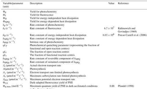
Appendix A: Leaf-level chlorophyll fluorescence model The leaf-level model for ChlF is based on work by Magnani and Dayyoub (2017). The definitions of the variables and pa-rameters and their possible numerical values and references are in Table A1.

Excitation energy that enters the leaf will be dissipated through photochemistry (subscript p), fluorescence (f), energy-independent (D) and energy-dependent heat dissipa-tion (NPQ) with the following yields (8)calculated with rate constantski:

8p= kp

kp+kf+kD+kNPQ

, (A1a)

8f= kf

kp+kf+kD+kNPQ

, (A1b)

8D=

kD

kp+kf+kD+kNPQ

, (A1c)

8NPQ=

kNPQ

kp+kf+kD+kNPQ. (A1d)

The rate constant of photochemistry (kp)can be expressed

as a function of the intrinsic rate of photochemistry (kPSII),

photochemical quenching parameter qLT (representing the fraction of functional and open reaction centres) consisting of qLr (the fraction of open reaction centres) and qLs (the

fraction of functional reaction centres, the sustained compo-nent of the photochemical quenching parameter):

kp=kPSII×qLT =kPSII×qLs×qLr. (A2) The rate constant for regulated thermal energy dissipation (kNPQ) consists of reversible component (NPQs) and sus-tained component (NPQr):

kNPQ=kNPQs+kNPQr. (A3)

The fluorescence and photochemistry yields can be ex-pressed by combining Eqs. (A1–A4):

8p=

kPSII×qLs×qLr

kPSII×qLs×qLr+kf+kD+kNPQr+kNPQs, (A4a) 8f=

kf

kPSII×qLs×qLr+kf+kD+kNPQr+kNPQs

, (A4b) and the ratio of these two gives

8p 8f

=kPSII

kf

×qLs×qLr. (A5)

The actual electron transportJais Ja=J (I )×

A Aj

, (A6)

where A is photosynthesis (minimum of the electron transport rate-limited photosynthesis Aj, and maximum

carboxylation rate-limited photosynthesis, Ac, in units µmol m−2_s−1_{),J is the electron transport shown in Eq. (2).}

TheJa is used in the calculation to describe the fraction of incoming quanta that is used for photosynthesis, i.e. the pho-tochemical quantum yield of photosystem II (PSII),8p

8p=Ja

I . (A7)

The rate of PSII reduction can be assumed to be proportional to the fraction of functional and closed reaction centres:

Ja=qLs×(1−qLr)×Jmax. (A8)

Therefore, the fraction of reaction centres that are functional and open is

qLs×qLr=qLs−I×8p

Jmax

. (A9)

By substituting Eqs. (A9) to (A5), the following expression for fluorescence yield is obtained:

8f,1=8p× kf kPSII

× 1

qLs− I×8p

Jmax

. (A10)

The rate constantkNPQis constant or close to zero in condi-tions of light-limited carboxylation (Walters et al., 1993), as energy-dependent heat dissipation is the result of pH build-up in the thylakoid lumen and xanthophyll de-epoxidation. From Eq. (A1b) and (A1d) the thermal energy dissipation in low light conditions is

8NPQ=8f× kNPQs

kf . (A11)

From Eq. (A1b) and (A1c) we obtain

8D=8f kD

kf. (A12)

Under these conditions a negative relationship between pho-tochemical and fluorescence yields is expected, since

8p=1−8f−8D−8NPQ

=1−8f−8f×kD

kf

−8fkNPQs kf

. (A13)

From this equation fluorescence yield at low light conditions can be derived to be

8f,2=(1−8p)×(

kf kf+kD+kNPQs

). (A14)

The fluorescence yield of PSII,8f, is taken as the minimum of8f,1and8f,2:

8f=min 8f,1, 8f,2

Table A1.Descriptions of the variables and parameters.

Variable/parameter Description Value Reference

(unit)

8p Yield for photochemistry

8f Yield for fluorescence

8D Yield for energy-independent heat dissipation

8NPQ Yield for energy-dependent heat dissipation

kp(s−1) Rate constant of photochemistry

kf(s−1) Rate constant of fluorescence 6.7×107 Rabinowich and

Govindjee (1969)

kD(s−1) Rate constant of energy-independent heat dissipation 6.03×108 Porcar-Castell et al. (2006)

kNPQ(s−1) Rate constant of energy-dependent heat dissipation

kPSII(s−1) Intrinsic rate of photochemistry

qLT Photochemical quenching parameter (representing the fraction of functional and open reaction centres)

qLr The fraction of open reaction centres qLs The fraction of functional reaction centres

kNPQr(s−1) Rate constant of reversible component ofkNPQ

kNPQs(s−1) Rate constant of sustained component ofkNPQ

Ja(µmol m−2s−1) Actual electron transport rate

A(µmol m−2s−1) Photosynthesis

Aj (µmol m−2s−1) Electron transport rate-limited photosynthesis

Ac(µmol m−2s−1) Maximum carboxylation rate-limited photosynthesis

Jmax(µmol m−2s−1) Maximum potential electron transport rate

8f,0 Dark-adapted fluorescence yield of PSII

8p,max(mol E−1) Maximum quantum yield of PSII in dark-acclimated conditions 0.88 Pfundel (1998)

in the absence of stress

The reference minimum fluorescence yield, obtained in dark-acclimated foliage in the absence of stress8f,0can be

the-oretically derived from the rate constant of fluorescencekf

(6.7×107s−1)(Rabinowich and Govindjee, 1969), the rate constant of thermal deactivationkD(6.03×108s−1_{)and the}

rate constant for photochemistry in open PSII reaction cen-treskPSIIas

8f,0=

kf kf+kPSII+kD

, (A16)

andkPSII(Genty et al., 1989) can be derived as kPSII=

(kD+kf)×8p,max (1−8p,max)

, (A17)

where8p,max(0.88 mol E−1) is the maximum quantum yield

of PSII in dark-acclimated conditions in the absence of stress obtained fluorometrically after correction for PSI fluores-cence (Pfundel, 1998).

To obtain the scaled fluorescence yield8f,s, the

fluores-cence yield8fis further divided by8f,0, 8f,s=

8f 8f,0

Appendix B: List of abbreviations

8f quantum yield of fluorescence (quanta emitted/quanta absorbed)

8f,s scaled quantum yield of fluorescence (quanta emitted/quanta absorbed)

8p quantum yield of photochemistry in PSII (electrons transported/quanta absorbed) ChlF chlorophyll fluorescence (general term)

ESM Earth System Model

EVI enhanced vegetation index

F0 prevailing fluorescence signal as measured with PAM fluorometry (relative units, e.g. sensor mV output)

fAPAR fraction of absorbed photosynthetic active radiation by vegetation FTS Fourier transform spectrometer; spectrometer on GOSAT satellite GOME-2 Global Ozone Monitoring Experiment-2; spectrometer on MetOp-A

(Meteorological Operational Satellites) satellite GOSAT Greenhouse Gases Observing Satellite GPP gross primary production

JSBACH Jena Scheme for Biosphere Atmosphere Coupling in Hamburg; the land surface model of the Max Planck Institute’s Earth System Model

LSM Land Surface Model

NDVI normalized difference vegetation index PAR photosynthetically active radiation

PSII photosystem II

SCIAMACHY SCanning Imaging Absorption SpectroMeter for Atmospheric CHartographY; spectrometer on ENVISAT (ENVIronmental SATellite) satellite

SCOPE Soil-Canopy Observation of Photosynthesis and Energy

The Supplement related to this article is available online at doi:10.5194/bg-14-1969-2017-supplement.

Author contributions. Tea Thum and S. Zaehle did the implementa-tion of the chlorophyll fluorescence model into the JSBACH model. Philipp Köhler and Luis Guanter provided remote sensing data. Mika Aurela and Tuomas Laurila provided the micrometeorolog-ical and meteorologmicrometeorolog-ical data for sites FI-Ken and FI-Sod. Annalea Lohila provided data for FI-Kns and Pasi Kolari for FI-Hyy. Fed-erico Magnani contributed the chlorophyll fluorescence model and Christiaan Van Der Tol the SCOPE model. Tiina Markkanen set up the regional model and prepared the meteorological forcing data for the model. Tea Thum did the simulations and analysed the data with help of the co-authors. Tea Thum prepared the manuscript with con-tributions from all co-authors.

Competing interests. Author Sönke Zaehle is a member of the edi-torial board of the journal.

Acknowledgements. Tea Thum acknowledges funding from the Academy of Finland (grant no. 266803). Sönke Zaehle was supported by the European Research Council (ERC) under the Eu-ropean Union’s Horizon 2020 research and innovation programme (QUINCY; grant no. 647204). We thank Thomas Kaminski for providing fAPAR data for all the regions and sites. Help from Leif Backman in acquisition of ERA-Interim data is acknowledged. We thank the Academy of Finland Centre of Excellence (grant nos. 1118615 and 272041). We thank Martin Jung for the use of the MPI-BGC GPP product. We are grateful to Albert Porcar-Castell for sharing his leaf-level ChlF data from Hyytiälä and for fruitful discussions. We thank Sophia Walther and Kristin Böttcher for their valuable comments on the manuscript. Two anonymous referees, whose comments greatly improved the manuscript, are gratefully acknowledged.

Edited by: G. Wohlfahrt

Reviewed by: two anonymous referees

References

Aurela M., Lohila A., Tuovinen J.-P., Hatakka J., Penttilä T., and Laurila, T.: Carbon dioxide and energy flux measurements in four northern-boreal ecosystems at Pallas, Boreal Env. Res., 20, 455– 473, 2015.

Baker, N. R.: Chlorophyll fluorescence: A probe of photosynthesis in vivo, Annu. Rev. Plant Biol., 59, 89–113, 2008.

Bergh, J., McMurtrie, R. E., and Linder, S.: Climatic factors control-ling the productivity of Norway spruce: a model-based analysis, Forest Ecol. Manag., 110, 127–139, 1998.

Bonan, G. B.: Forests and climate change: Forcings, feedbacks, and the climate benefits of forests, Science, 320, 1444–1449, 2008. Böttcher K., Aurela, M., Kervinen, M., Markkanen, T., Mattila,

O.-P., Kolari, O.-P., Metsämäki, S., Aalto, T., Arslan, A., and Pulliainen, J.: MODIS time-series-derived indicators for the beginning of

the growing season in boreal coniferous forest – A comparison with CO2flux measurements and phenological observations in

Finland, Remote Sens. Environ., 140, 625–638, 2014.

Collatz, G. J., Ribas-Carbo, M., and Berry, J. A.: Cou-pled photosynthesis-stomatal conductance model for leaves of C4 plants, Aust. J. Plant Physiol., 19, 519–538, doi:10.1071/PP9920519, 1992.

Dee, D. P., Uppala, S. M., Simmons, A. J., Berrisford, P., Poli, P., Kobayashi, S., Andrae, U., Balmaseda, M. A., Balsamo, G., Bauer, P., Bechtold, P., Beljaars, A. C. M., van de Berg, L., Bid-lot, J., Bormann, N., Delsol, C., Dragani, R., Fuentes, M., Geer, A. J., Haimberger, L., Healy, S. B., Hersbach, H., Hólm, E. V., Isaksen, L., Kållberg, P., Köhler, M., Matricardi, M., McNally, A. P., Monge-Sanz, B. M., Morcrette, J.-J., Park, B.-K., Peubey, C., de Rosnay, P., Tavolato, C., Thépaut, J.-N., and Vitart, F.: The ERA-Interim reanalysis: configuration and performance of the data assimilation system, Q. J. R. Meteorol. Soc., 137, 553–597, 2011.

Dickinson, R. E.: Land surface processes and climate-surface albe-dos and energy balance, Adv. Geophys., 25, 305–353, 1983. Farquhar G. D., von Caemmerer S., and Berry J. A.: A

biogeochem-ical model of photosynthesis in leaves of C3 species, Planta, 149, 78–90, 1980.

Frankenberg, C., Fisher, J. B., Worden, J., Badgley, G., Saatchi, S. S., Lee, J.-E., Toon, G. C., Butz, A., Jung, M., Kuze, A., and Yokota, T.: New global observations of the terrestrial car-bon cycle from GOSAT: Patterns of plant fluorescence with gross primary productivity, Geophys. Res. Lett., 38, L17706, doi:10.1029/2011GL048738, 2011.

Frankenberg, C., O’Dell, C., Berry, J., Guanter, L., Joiner, J., Köh-ler, P., Pollock, R., and Taylor, T. E.: Prospects for chloro-phyll fluorescence remote sensing from the Orbiting Carbon Observatory-2, Remote Sens. Environ., 147, 1–12, 2014. Giorgetta M. A., Jungclaus, J., Reick, C. H., Legutke, S., Bader,

J., Böttinger, M., Brovkin, V., Crueger, T., Esch, M., Fieg, K., Glushak, K., Gayler, V., Haak, H., Hollweg, H.-D., Ilyina, T., Kinne, S., Kornblueh, L., Matei, D., Mauritsen, T., Mikolajew-icz, U., Mueller, W., Notz, D., Pithan, F., Raddatz, T., Rast, S., Redler, R., Roeckner, E., Schmidt, H., Schnur, R., Segschnei-der, J., Six, K. D., Stockhause, M., Timmreck, C., Wegner, J., Widmann, H., Wieners, K.-H., Claussen, M., Marotzke, J., and Stevens, B.: Climate and carbon cycle changes from 1850 to 2100 in MPI-ESM simulations for the Coupled Model Intercom-parison Project phase 5, J. Adv. Model. Earth Syst., 5, 572–597, 2013.

Guanter, L., Frankenberg, C., Dudhia, A., Lewis, P. E., Gómez-Dans, J., Kuze, A., Suto, H., and Grainger, R. G.: Retrieval and global assessment of terrestrial chlorophyll fluorescence from GOSAT space measurements, Remote Sens. Environ., 121, 236– 251, doi:10.1016/j.rse.2012.02.006, 2012.

Guanter, L., Aben, I., Tol, P., Krijger, J. M., Hollstein, A., Köhler, P., Damm, A., Joiner, J., Frankenberg, C., and Landgraf, J.: Poten-tial of the TROPOspheric Monitoring Instrument (TROPOMI) onboard the Sentinel-5 Precursor for the monitoring of terrestrial chlorophyll fluorescence, Atmos. Meas. Tech., 8, 1337–1352, doi:10.5194/amt-8-1337-2015, 2015.

Jacob, D.: A note to the simulation of the annual and inter-annual variability of the water budget over the Baltic Sea drainage basin, Meteorol. Atmos. Phys., 77, 61–73, 2001.

Jacob, D. and Podzun, R.: Sensitivity studies with the regional cli-mate model REMO, Meteorol. Atmos. Phys., 63, 119–129, 1997. Jacob, D., Van den Hurk, B. J. J. M., Andrae, U., Elgered, G., Fortelius, C., Graham, L. P., Jackson, S. D., Karstens, U., Köp-ken, Chr., Lindau, R., Podzun, R., Rockel, B., Rubel, F., Sass, B. H., Smith, R. N. B., and Yang, X.: A comprehensive model inter-comparison study investigating the water budget during the BALTEX-PIDCAP period, Meteorol. Atmos. Phys., 77, 19–43, 2001.

Joiner, J., Guanter, L., Lindstrot, R., Voigt, M., Vasilkov, A. P., Middleton, E. M., Huemmrich, K. F., Yoshida, Y., and Franken-berg, C.: Global monitoring of terrestrial chlorophyll fluores-cence from moderate-spectral-resolution near-infrared satellite measurements: methodology, simulations, and application to GOME-2, Atmos. Meas. Tech., 6, 2803–2823, doi:10.5194/amt-6-2803-2013, 2013.

Joiner, J., Yoshida, Y., Vasilkov, A. P., Yoshida, Y., Corp, L. A., and Middleton, E. M.: First observations of global and seasonal terrestrial chlorophyll fluorescence from space, Biogeosciences, 8, 637–651, doi:10.5194/bg-8-637-2011, 2011.

Joiner, J., Yoshida, Y., Vasilkov, A. P., Middleton, E. M., Camp-bell, P. K. E., Yoshida, Y., Kuze, A., and Corp, L. A.: Filling-in of near-infrared solar lines by terrestrial fluorescence and other geo-physical effects: simulations and space-based observations from SCIAMACHY and GOSAT, Atmos. Meas. Tech., 5, 809–829, doi:10.5194/amt-5-809-2012, 2012.

Joiner, J., Yoshida, Y., Vasilkov, A. P., Schaefer, K., Jung, M., Guanter, L., Zhang, Y., Garrity, S., Middleton, E. M., Huemm-rich, K. F., Gu, L., and Belelli Marchesini, L.: The seasonal cycle of satellite chlorophyll fluorescence observations and its relationship to vegetation phenology and ecosystem atmo-sphere carbon exchange, Remote Sens. Environ., 152, 375–391, doi:10.1016/j.rse.2014.06.022, 2014.

Jung, M., Reichstein, M., and Bondeau, A.: Towards global em-pirical upscaling of FLUXNET eddy covariance observations: validation of a model tree ensemble approach using a biosphere model, Biogeosciences, 6, 2001–2013, doi:10.5194/bg-6-2001-2009, 2009.

Jung, M., Reichstein, M., Margolis, H. A., Cescatti, A., Richard-son, A. D., Arain, M. A., Arneth, A., Bernhofer, C., Bonal, D., Chen, J. Gianelle, D., Gobron, N., Kiely, G., Kutsch, W., Lass-lop, G., Law, B. E., Lindroth, A., Merbold, L., Montagnani, L., Moors, E. J., Papale, D., Sottocornola, M., Vaccari, F., and Williams, C.: Global patterns of land-atmosphere fluxes of car-bon dioxide, latent heat, and sensible heat derived from eddy co-variance, satellite, and meteorological observations, J. Geophys. Res., 116, G00J07, doi:10.1029/2010JG001566, 2011.

Koffi, E. N., Rayner, P. J., Norton, A. J., Frankenberg, C., and Scholze, M.: Investigating the usefulness of satellite derived flu-orescence data in inferring gross primary productivity within the carbon cycle data assimilation system, Biogeosciences 12, 4067– 4084, doi:10.5194/bg-12-4067-2015, 2015.

Köhler, P., Guanter, L., and Joiner, J.: A linear method for the re-trieval of sun-induced chlorophyll fluorescence from GOME-2 and SCIAMACHY data, Atmos. Meas. Tech., 8, 2589–2608, doi:10.5194/amt-8-2589-2015, 2015.

Kolari, P.: Meteorological and CO2flux data for FI-Hyy,

Univer-sity of Helsinki, http://avaa.tdata.fi/openida/dl.jsp?pid=urn:nbn: fi:csc-ida-2x201611242015017385197s last access: 14 January 2014.

Kolari, P., Kulmala, L., Pumpanen, J., Launiainen, S., Ilvesniemi, H., Hari, P., and Nikinmaa, E.: CO2 exchange and component

CO2fluxes of a boreal Scots pine forest, Boreal Environ. Res.,

14, 761–783, 2009.

Kolari, P., Chan, T., Porcar-Castell, A., Bäck, J., Nikinmaa, E., and Juurola, E.: Field and controlled environment measurements show strong seasonal acclimation in photosynthesis and respi-ration potential in boreal Scots pine, Front. Plant Sci., 5, 717, doi:10.3389/fpls.2014.00717, 2014.

Knorr, W.: Annual and interannual CO2exchanges of the terrestrial

biosphere: process-based simulations and uncertainties, Global Ecol. Biogeogr., 9, 225–252, 2000.

Krivosheeva, A., Tao, D. L., Ottander, C., Wingsle, G., Dube, S. L., and Öquist, G.: Cold acclimation and photoinhibition of photo-synthesis in Scots pine, Planta, 200, 296–305, 1996.

Lansø, A. S.: Mesoscale modelling of atmospheric CO2across

Den-mark, PhD thesis, Aarhus University, DenDen-mark, 2016.

Le Quéré, C., Andrew, R. M., Canadell, J. G., Sitch, S., Kors-bakken, J. I., Peters, G. P., Manning, A. C., Boden, T. A., Tans, P. P., Houghton, R. A., Keeling, R. F., Alin, S., Andrews, O. D., Anthoni, P., Barbero, L., Bopp, L., Chevallier, F., Chini, L. P., Ciais, P., Currie, K., Delire, C., Doney, S. C., Friedlingstein, P., Gkritzalis, T., Harris, I., Hauck, J., Haverd, V., Hoppema, M., Klein Goldewijk, K., Jain, A. K., Kato, E., Körtzinger, A., Land-schützer, P., Lefèvre, N., Lenton, A., Lienert, S., Lombardozzi, D., Melton, J. R., Metzl, N., Millero, F., Monteiro, P. M. S., Munro, D. R., Nabel, J. E. M. S., Nakaoka, S.-I., O’Brien, K., Olsen, A., Omar, A. M., Ono, T., Pierrot, D., Poulter, B., Röden-beck, C., Salisbury, J., Schuster, U., Schwinger, J., Séférian, R., Skjelvan, I., Stocker, B. D., Sutton, A. J., Takahashi, T., Tian, H., Tilbrook, B., van der Laan-Luijkx, I. T., van der Werf, G. R., Viovy, N., Walker, A. P., Wiltshire, A. J., and Zaehle, S.: Global Carbon Budget 2016, Earth Syst. Sci. Data, 8, 605–649, doi:10.5194/essd-8-605-2016, 2016.

Lee, J.-E., Berry, J. A., van der Tol, C., Yang, X., Guanter, L., Damm, A., Baker, I., and Frankenberg, C.: Simulations of chlorophyll fluorescence incorporated into the Community Land Model version 4, Glob. Change Biol., 21, 3469–3477, doi:10.1111/gcb.12948, 2015.

Lohila, A., Minkkinen, K., Aurela, M., Tuovinen, J.-P., Penttilä, T., Ojanen, P., and Laurila, T.: Greenhouse gas flux measurements in a forestry-drained peatland indicate a large carbon sink, Bio-geosciences, 8, 3203–3218, doi:10.5194/bg-8-3203-2011, 2011. Luo, Y. Q., Randerson, J. T., Abramowitz, G., Bacour, C., Blyth, E., Carvalhais, N., Ciais, P., Dalmonech, D., Fisher, J. B., Fisher, R., Friedlingstein, P., Hibbard, K., Hoffman, F., Huntzinger, D., Jones, C. D., Koven, C., Lawrence, D., Li, D. J., Mahecha, M., Niu, S. L., Norby, R., Piao, S. L., Qi, X., Peylin, P., Prentice, I. C., Riley, W., Reichstein, M., Schwalm, C., Wang, Y. P., Xia, J. Y., Zaehle, S., and Zhou, X. H.: A framework for benchmarking land models, Biogeosciences, 9, 3857–3874, doi:10.5194/bg-9-3857-2012, 2012.

chlorophyll fluorescence: Review of methods and applications, Remote Sens. Environ., 113, 2037–2051, 2009.

Magnani, F. and Dayyoub, A.: Modelling chlorophyll fluorescence under ambient conditions, in preparation, 2017.

Mammarella I., Launiainen S., Grönholm T., Keronen P., Pumpanen J., Rannik, Ü., and Vesala, T.: Relative humidity effect on the high frequency attenuation of water vapour flux measured by a closed-path eddy covariance system, J. Atmos. Ocean Tech., 26, 1856–1866, 2009.

Markkanen, T., Thum, T., Susiluoto, J., Aurela, M., Gao, Y., Laurila, T., Lehtonen, A., Liski, J., Lohila, A., Mammarella, I., ˇTupek, B., and Aalto, T.: Modelling carbon fluxes and pools in Finland and their trends in past decades, in preparation, 2017.

Maxwell, K. and Johnson, G. N.: Chlorophyll fluorescence – a prac-tical guide, J. Exp. Bot., 61, 659–668, 2000.

Munro, R., Eisinger, M. Anderson, C., Callies, J., Corpaccioli, E., Lang, R., Lefebvre, A., Livschitz, Y., and Perez Albinana, A.: GOME-2 on MetOp: from in-orbit verification routine to routine operations, in: Proceeding of EUMETSAT Meteorological Satel-lite Conference, Helsinki, Finland, 12–16 June 2006.

Murchie, E. H. and Lawson, T.: Chlorophyll fluorescence analysis: a guide to good practice and understanding some new applications, J. Exp. Bot., 64, 3983–3998, doi:10.1093/jxb/ert208, 2013. Norton, A. J., Rayner, P. J., Koffi, E. N., and Scholze, M.:

Assim-ilating solar-induced chlorophyll fluorescence into the terrestrial biosphere model BETHY-SCOPE: Model description and infor-mation content, Geosci. Model Dev. Discuss., doi:10.5194/gmd-2017-34, in review, 2017.

Parazoo, N. C., Bowman, K., Frankenberg, C., Lee, J.-E., Fisher, J. B., Worden, J., Jones, D. B. A., Berry, J., Collatz, G. J., Baker, I. T., Jung, M., Liu, J., Osterman, G., O’Dell, C., Sparks, A., Butz, A., Guerlet, S., Yoshida, Y., Chen, H., and Gerbig, C.: In-terpreting seasonal changes in the carbon balance of southern Amazonia using measurements of XCO2 and chlorophyll

flu-orescence from GOSAT, Geophys. Res. Lett., 40, 2829–2833, doi:10.1002/grl.50452, 2013.

Parazoo, N. C., Bowman, K., Fisher, J. B., Frankenberg, C., Jones, D. B. A., Cescatti, A., Pérez-Priego, Ó., Wohlfahrt, G., and Mon-tagnani, L.: Terrestrial gross primary production inferred from satellite fluorescence and vegetation models, Glob. Change Biol., 20, 3103–3121, doi:10.1111/gcb.12652, 2014.

Palmroth, S. and Hari, P.: Evaluation of the importance of acclima-tion of needle structure, photosynthesis, and respiraacclima-tion to avail-able photosynthetically active radiation in a Scots pine canopy, Can. J. For. Res., 31, 1235–1243, 2001.

Pinty, B., Clerici, M., Andredakis, I., Kaminski, T., Taberner, M., Verstraete, M. M., Gobron, N., Plummer, S., and Widlowski, J.-L.: Exploiting the MODIS albedos with the Two-stream In-version Package (JRC-TIP): 2. Fractions of transmitted and ab-sorbed fluxes in the vegetation and soil layers, J. Geophys. Res., 116, D09106, doi:10.1029/2010JD015373, 2011.

Porcar-Castell, A., Bäck, J., Juurola, E., and Hari, P.: Dynamics of the energy flow through photosystem II under changing light conditions: a model approach, Funct. Plant Biol., 33, 229–239, 2006.

Porcar-Castell, A., Pfündel, E., Korhonen, J. F. J., and Juurola, E.: A new monitoring PAM fluorometer (MONI-PAM) to study the short- and long-term acclimation of photosystem II in field con-ditions, Photosynth. Res., 96, 173–179, 2008.

Porcar-Castell, A.: A high resolution portrait of the annual accli-mation in photochemical and non-photochemical quenching in needles of Pinus sylvestris, Physiol. Plantarum, 143, 139–153, 2011.

Porcar-Castell, A., Tyystjärvi, E., Atherton, J., van der Tol, C., Flexas, J., Pfündel, E., Moreno, J., Frankenberg, C., and Berry, J. A.: Linking chlorophyll-a fluorescence to photosynthesis for re-mote sensing applications: mechanisms and challenges, J. Exp. Bot., 65, 4065–4095 doi:10.1093/jxb/eru191, 2014.

Rabinowich, E. and Govindjee: Photosynthesis, John Wiley and Sons, New York, 273 pp., 1969.

Rannik, Ü., Keronen, P., Hari, P., and Vesala, T.: Estimation of forest-atmosphere CO2exchange by eddy covariance and profile

techniques, Agr. Forest Meteorol., 126, 141–155, 2004. Rannik, Ü., Peltola, O., and Mammarella, I.: Random

uncertain-ties of flux measurements by the eddy covariance technique, At-mos. Meas. Tech., 9, 5163–5181, doi:10.5194/amt-9-5163-2016, 2016.

Reick, C. H., Raddatz, T., Brovkin, V., and Gayler, V.: Represen-tation of natural and anthropogenic land cover change in MPI-ESM, J. Adv. Model. Earth Syst., 5, 459–482, 2013.

Ruosteenoja, K., Raisanen, J., and Pirinen, P.: Projected changes in thermal seasons and the growing season in Finland, Int. J. Cli-matol., 31, 1473–1487, 2011.

Schaefer, K., Schwalm, C. R., Williams, C., Arain, M. A., Barr, A., Chen, J. M., Davis, K. J., Dimitrov, D., Hilton, T. W., Hollinger, D. Y., Humphreys, E., Poulter, B., Raczka, B. M., Richardson, A. D., Sahoo, A., Thornton, P., Vargas, R., Verbeeck, H., An-derson, R., Baker, I., Black, T. A., Bolstad, P., Chen, J., Cur-tis, P. S., Desai, A. R., Dietze, M., Dragoni, D., Gough, C., Grant, R. F., Gu, L., Jain, A., Kucharik, C., Law, B., Liu, S., Lokipitiya, E., Margolis, H. A., Matamala, R., McCaughey, J. H., Monson, R., Munger, J. W., Oechel, W., Peng, C., Price, D. T., Ricciuto, D., Riley, W. J., Roulet, N., Tian, H., Tonitto, C., Torn, M., Weng, E., and Zhou, X.: A model-data comparison of gross primary productivity: Results from the North American Carbon Program site synthesis, J. Geophys. Res., 117, G03010, doi:10.1029/2012JG001960, 2012.

Sellers, P. J.: Canopy reflectance, photosynthesis and transpiration, Int. J. Remote Sens., 6, 1335–1372, 1985.

Sitch, S., Friedlingstein, P., Gruber, N., Jones, S. D., Murray-Tortarolo, G., Ahlström, A., Doney, S. C., Graven, H., Heinze, C., Huntingford, C., Levis, S., Levy, P. E., Lomas, M., Poulter, B., Viovy, N., Zaehle, S., Zeng, N., Arneth, A., Bonan, G., Bopp, L., Canadell, J. G., Chevallier, F., Ciais, P., Ellis, R., Gloor, M., Peylin, P., Piao, S. L., Le Quéré, C., Smith, B., Zhu, Z., and Myneni, R.: Recent trends and drivers of regional sources and sinks of carbon dioxide, Biogeosciences, 12, 653– 679, doi:10.5194/bg-12-653-2015, 2015.

Thum, T., Aalto, T., Laurila, T., Aurela, M., Kolari, P., and Hari, P.: Parametrization of two photosynthesis models at the canopy scale in a northern boreal Scots pine forest, Tellus B, 59, 874– 890, 2007.

Thum, T., Aalto, T., Laurila, T., Aurela, M., Lindroth, A., and Vesala, T.: Assessing seasonality of biochemical CO2exchange