Translation of Extended Petri Net Model into Ladder
Diagram and Simulation with PLC
Tomaž Perme
DRP Perme Tomaž, s. p., Slovenia
University of Primorska, Faculty of Management Koper, Slovenia
Modelling and simulation can significantly help with the teaching and learning of PLC programming, training of the operators and maintaining personal, developing automated systems and diagnosis of the systems’ operation. The basic idea of the presented research and development was to use PLC programming tool for modelling a discrete mechatronic system and simulate its operation on industrial PLC or on emulation of PLC on the PC computer.
For the realization of the idea the extensions of the basic Petri net theory (EPN) and direct translation of the EPN model into the ladder diagram were elaborated, which enabled the use of the EPN model for simulation on PLC. Furthermore, the building blocks of EPN model were developed within the programme for discrete simulation, which enable building and verification of an EPN model of the observed system within the programme for discrete simulation before its implementation.
The primary test of the method and the usability verification of the basic idea show that the method is applicable for teaching and learning of PLC programming and can also be used for an advanced developing and testing of PLC programmes.
© 2009 Journal of Mechanical Engineering. All rights reserved.
Keywords: extended Petri net, ladder diagram, PLC, modelling, simulation, electro-pneumatic systems, discrete mechatronic systems
0 INTRODUCTION
The electro-pneumatic systems form a great portion of automation in bulk production and internal logistics. They are usually composed of mechanical construction, pneumatic or electrical drives, electrical sensors and programmable logical controllers (PLC). So the knowledge about the operation and programming of PLCs became essential for mechanical, electrical or mechatronic engineers that develop, design, control, maintain, modernize or only operate automated production systems. That is why modern curriculum on automation and mechatronics has to include practical courses of PLC programming, where students have to aquire as much practical experience as possible. The best experience can be obtained with hands-on real industrial equipment. But experience from practical courses shows that the equipment in laboratories and classrooms is always in some way a bottleneck. Therefore, new modern techniques like simulation have to be implemented and used complementary to and in cooperation with the real industrial equipment. That was the first issue in the realisation of the
idea about using industrial PLC and PC emulation of industrial PLC for simulation.
control programme regarding the requirements of the system’s operation. The variables can be changed by a simulation part of the PLC programme that represents the dynamic model of the controlled system.
This was the background for developing the concept of simulation of electro-pneumatic systems with the industrial PLC controller. New to the concept is the idea of successive execution of the control and simulation part of the PLC programme on a real or virtual PLC controller. Students and engineers can write the control programme for the PLC controller with an industrial PLC programming tool and verify its correctness and functionality in a completely industrial environment.
Although the idea of using a part of the PLC programme for a simulation model is very simple, the realisation encountered a significant challenge. The usefulness of the idea completely depends on accuracy of the simulation model, i.e. simulation part of PLC programme. First attempts to translate a formal model of double-acting pneumatic cylinder controlled by a 4/2-way valve into a ladder diagram pointed out the difficulty of accurate modelling as well as the verification and validation of the simulation model within the tool for PLC programming. PLC programme is primarily intended to control the system in the space of desired states according to the specified algorithm. On the contrary, the simulation model has to include all possible or reachable states of the system. In an advanced simulation model also unexpected states of the system like failures have to be considered as a part of the possible state space of the system.
The paper presents the realisation of the idea that is the result of the author’s research and development on virtual environment [6] and remote laboratory [7] for education and training [8] as well as the implementation of Petri net for modelling and simulation as support for planning of production systems [9] to [11]. For the realization of the idea the basic theory of Petri net was extended in a way that the operation and control of electro-pneumatic systems can be modelled. The EPN model is then translated according to the elaborated rules into the ladder diagram. The translation enables using the EPN model of the system with the control algorithm for simulation on PLC or emulation of PLC.
1 SIMULATION USING PROGRAMMABLE LOGICAL CONTROLLER
A model of the system can be used for several purposes. The model is most of all needed in the design stage of a new system or for a re-design of an existent system [9] or a system component [12] for obtaining its structure and dynamic behaviour. The model is also used for planning [13] or control and diagnostic purposes [3]. The model can also be used as a platform for education and training [6]. In all these cases the model has to be a reliable and consistent representation of the real system. The transformation of the elements of the observed system and the relations between them into the data space has to be comprehensible to the engineer as well as to the machine. The engineer needs to define their requirements and requests in a form of instructions, on the basis of which the machine can operate and fulfil the required functionality.
1.1 The Concept of Simulation with the PLC Programme
Simulation is a method and a tool for obtaining the structure and dynamic behaviour of the observed system, which cannot be obtained with other methods and tools in an economical way or in acceptable time frame. Usually the development of PLC programmes does not include simulation, so the PLC programme is tested only after the system is installed.
Already at the design stage of the system most data for the modelling and simulation are available including a required operation of the system and the functionality of the control programme, But the simulation is still not used to help to develop error-free PLC programme. Because the users do not expect the simulation support from the programming tools, most PLC providers have not included simulation in their programming tools, at least not directly.
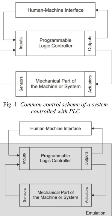
PLC reads the state of the inputs cyclically, so the response from the real system has to be permanent. This can be achieved with the two parts of the PLC programme that is running on the real PLC or in the emulation of PLC on a PC. First part is the control programme that controls the machine or system. The second part of the PLC programme reads the inputs, simulates the behaviour of controlled machine or system and writes the outputs. This means that the simulation part of the programme changes the state of the inputs to the control programme on the basis of the set outputs: This is done in the same way and the real system does that by means of the sensors and actuators (Fig. 2).
Fig. 1. Common control scheme of a system controlled with PLC
Fig. 2. Control scheme of a simulation with PLC
Simulation with the PLC has some advantages, but also some limitations. The main
advantage is that the control part of the PLC programme is the same as the PLC programme that will control the real system. The limitations are mostly related to the characteristics of PLC controllers like limited internal memory and so the size of the simulation model, speed of the processor and so the time for execution of the simulation, and specificity of the PLC programming languages.
The first two limitations can be solved with a more powerful PLC, programmable automation controllers (PAC) or with the emulation of PLC on PCs. Emulation refers to the ability of a computer program or electronic device to imitate another program or device. An emulator duplicates the functions of one system using a different system, so that the second system behaves like the first system. This means that the PLC programme developed for a particular type or a particular PLC controller can also run on the PC. If the PLC programme also includes the simulation part, the control part of the PLC programme can be tested and so errors can be identified and removed.
1.2 PLC Programming Languages
The PLC programming languages are also the encountered modelling limitation. There are five programming languages for PLCs defined in the IEC 61131 standard. The instruction list (IL) is the first textual and ladder diagram (LD), the first graphical PLC programming language. LD is still most frequently used in all kinds of PLC devices. Both languages are based on the logic of relay control, which is still the basic logic of PLC devices. The next graphical programming language are function block diagram (FBD) and sequential function chart (SFC), which are used for higher level programming. Advanced textual PLC programming language is structured text (ST), which is very similar to the programming language Pascal. The advantage of graphical languages in comparison to textual is mostly the graphical interface that allows a visualisation of PLC programme execution and is more user friendly for programming [1] and [3].
- is the most frequently used PLC programming language and is available in practically all PLCs,
- offers a comprehensible and understandable description of operation that is based on relay logic and bool algebra,
- is very convenient for sequential algorithms on low operation level,
- comprehends graphical way of programming
and
- enables a visualisation of programme
execution.
More complicated than just selecting an appropriate programming language was solving the specificity and adequacy of the PLC programming language including the ladder diagram for building the simulation model. The fact is that the programming languages are aimed for the building of the control programmes and not for the modelling of the processes and systems under control.
The described modelling problem can be solved with an appropriate modelling tool that also enables the translation of the model into the PLC programme. Many PN-based methods and tools have already proved the PN capability and competence for the modelling and control design of discrete-event systems as well as a translation of PN-based control sequence into ladder diagram or sequential function chart (IEC 61131-3) [14] to [17]. The PN also has good mathematical background [18] and [19] and an inherited graphic presentation that features great modelling, analysing and simulation capabilities [20].
2 PETRI NET AND LADDER DIAGRAM
The electro-pneumatic components for automated assembly and handling devices are typical systems where properties are changed in discrete points in time. Such systems are described as discrete-event systems and can be modelled with Petri nets. But for different applications there are also different modelling requirements.
2.1 Requirements on Petri Net Extensions
For the control of a discrete system we have to know the state of the system and the way how to move the system in certain time into next required state. For example, the pneumatic 2-axes
handling device has four end positions that form the state space of the system. The movement of the pneumatic cylinders changes these states according to the control sequence written in the control programme that makes the controller send signals to the solenoid valve of the pneumatic cylinder. In normal operation conditions and with an error free control programme the states of the valves that directly control the movement of the pneumatic cylinders is not important to know. But for the simulation, the consistent model of the valve-cylinder system is fundamental. There are also several internal states in the valve-cylinder system and the duration of the activities that have to be put into a model, and that with the basic theory of Petri net cannot be accurately modelled. Another reason for PN extensions is the adequate translation of PN model to the PLC programme written in the ladder diagram. The ladder diagram consists of elements and relations between them. The basic elements are input, output and internal variables, timers and counters. The main relations between these elements are AND, OR and NOT operand of Boolean algebra. The combination of elements and relations forms the statements that have not always an adequate representation within the basic theory of Petri net. Besides the negation there is also a lack of proper interpretation of input variables of LD in the PN model. In the ladder diagram the input variable does not change the state when the programme is executed. In PN model, however, the execution of enabled transition takes a corresponding number of tokens from input places and so it changes the state of the input places.
These requirements define the extensions of Petri net, which are negation of condition, signal connection and time transition.
2.2 Theoretical Background of Petri Nets Extensions
The formal definition of a Petri net [18] and [19] with the finite capacity (place/transition net) [20] extended with negation, signal connection and time is given by as an 6-tuple C = (P, T, F, W, M, Z) where:
P = { p1, p2, ...pm} is a finite set of places, T = {t1, t2, ...tn} is a finite set of transitions,
P∩T = 0 in P∪T≠ 0
F = Fs∪Fiin Fs∩Fi = 0
W: F→ {-1, 1} is a weight function,
M0: P→ {0, 1} is the initial marking,
Z: T → {0,1,2,3,..} defines the time for each transition.
The rule for transition enabling and firing is an execution rule, which can be described for an EPN in the:
• ts := {p | (p,t) ∈Fs} is a set of input places with
normal connections to the transition t,
ts•:= {p | (t,p) ∈Fs} is a set of output places with
normal connections to the transition t,
• ti: = {p | (p,t) ∈Fi} is a set of input places with
signal connections to the transition t,
ti•: = {p | (t,p) ∈Fi} is a set of output places with
signal connections to the transition t,
• t = • ts∪• ti is a set of input places of transition t
and
t•:= ts•∪ti• is a set of output places of transition t.
A transition t is enabled under marking M, if:
( ) 1 ( , ) 1 :
( ) 0 ( , ) 1 ,
M p W p t
p t
M p W p t
⎧ = ∀ =
⎪⎪ ∀ ∈ • ⎨⎪
= ∀ = −
⎪⎩ (1)
( ) 0 ( , ) 1 :
( ) 1 ( , ) 1 .
M p W t p
p t
M p W t p
⎧ = ∀ =
⎪⎪ ∀ ∈ • ⎨⎪
= ∀ = −
⎪⎩ (2)
Eq. (1) means that each input place to the transition t should be marked or not marked, if
w(p, t) is 1 and 0 respectively. Eq. (2) means that the output places of the transition t should not be marked, if w(p, t) is 1, or should be marked, if
w(p, t) is -1. Negative weight actually means negation. EPN does not solve nor envisage conflict situations and mutual exclusions which remain the subject of modelling.
Subset of transitions T’ ⊆ T is enabled under marking M, if ∀t∈T’ is enabled under the marking M.
If a transition is enabled and its time is null, it can fire. An enabled transition can fire depending on the duration of the transition in two ways. Zero-time transitions (z(t) = 0) fire completely at once and change the state according to
( ) ( , ) \ ,
( ) ( , ) \ ,
'( ) .
( ) ( , ) ( , ) ,
( ) else.
s s
s s
s s
M p W p t p t t
M p W t p p t t
M p
M p W p t W t p p t t
M p
⎧ − ∀ ∈• •
⎪⎪
⎪⎪ + ∀ ∈ • •
⎪⎪ =⎨⎪
− + ∀ ∈ •∩• ⎪⎪
⎪⎪⎪⎩ (3)
A firing of an enabled transition t removes one token from each input place p of transition t,
and adds one token to each output place p of transition t. This is true for each place p that is connected to the transition t with the normal
connection. For places p connected to the
transition t with signal connection, nothing is changed during the firing of transition t.
Nonzero-time transitions (z(t) > 0) fire in two steps. In the first step enabled transition t is added to the T-, where T- is a set of enabled
nonzero-time transitions {(t1, d1) (t2, d2)....(tn, dn)}
with elements (tk, dk), tk∈ T in dk∈ {1,2,3...},
where tk are enabled but not jet fired nonzero-time
transitions and dk their remaining times to firing.
In the second step the nonzero-time transition fires to the end. Firing to the end of nonzero-time transition tk happens when the
remaining time dk = 0 and the conditions (1) and
(2) are fulfilled (transition t is still enabled). Practically fires of the transition with the smallest remaining time dk:
∀(t,d)∈T- | t
k≠t : dk≤d. (4)
Firing to the end of enabled (1) (2) nonzero-time transition t from T- under M is
executed in the same way as firing of the normal transitions (3), where:
t = tk| (tk, dk) ∈T-. (5)
T-’ = T-\{(t
k, dk)} (6)
(t,d)’ = (t, d - dk)for∀(t,d) ∈T-’. (7)
Firing to the end of nonzero-time transition t means removing tokens from input places and adding tokens to the output places of transition t (3), removing elements (tk, dk) from T
-(6) and subtracting dk from d of all elements in T-
(7). Removing the element (tk, dk) from T-(6) is
executed also for the transition t (5) when they are not enabled any more. Nonzero-time transition can be in the same moment only in one element (tk, dk).
2.3 Gaphical Representation and Explanations of PN Extensions
place is the input or output place of a transition. If the arc between a place and a transition is bi-directed, the place is input and also output to that transition.
An arc directed from a place to a transition practically means a condition that has to be fulfilled for the transition to fire. The fulfilled condition is represented by a token in the place that represents the condition. In a graphical representation the tokens are represented by dots. An arc directed from a transition to a place means the consequence of the transition execution. When a transition fires, one token is removed from each input place and one token is put to each output place. All nodes are usually named, so the graph as well as the model is more comprehensible.
The negation of the condition defined by negative weighted function is graphically represented by an arc directed from a place to a transition and with a circle instead of an arrow at its end. The negation means that the transition is enabled if the condition is not fulfilled and the input place has no tokens. This corresponds to the negation in the ladder diagram.
The informational arc is graphically represented by a dashed line. The only difference between an informational and normal arc is that the informational arc leaves tokens in the connected input places when the corresponding transition fires. So the tokens remain in the places and the condition is still fulfilled. This is the case of the input signals on the PLC. The informational arc directed from a transition to a place has no practical meaning.
In real systems activities and processes need some time for execution and cannot be properly modelled by a transition that fires instantaneously. It is for this reason that time transition which does not fire instantaneously is introduced. Time transition actually fires in two steps. In the first step, only the condition fulfilment is verified. If the transition is still enabled after the elapsed time, it fires to the end like an ordinary transition. So the EPN model comprises of ordinary and time transitions. Time transition is usually represented by a larger rectangle, but in the continuation the ordinary and time transitions will have the same representation. We will distinguish between them only when we translate the EPN model to the ladder diagram.
2.4 Translation Rules of Extended Petri Net Model into the Ladder Diagram
EPN model is translated into the ladder diagram according to the developed rules. These rules define the interpretation of EPN definition in LD syntax:
- Each place in the EPN model has an internal or external one-bit (Boolean) variable in the LD. An EPN place that represents a control signal for the actuator or the signal from the sensor is translated into an external one-bit variable. External variables on real PLC are mapped to the physical output or input. Other EPN places are represented in LD by internal variables.
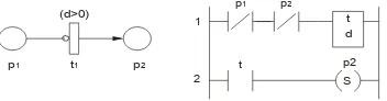
- Each EPN transition denotes one or two
statements i.e. rungs in the ladder diagram. Nonzero-time transition (time d is greater than zero) has two rungs in LD. The first rung contains a translation of enabling conditions and a timer with the switching time d. The second rung comprises the output variable from the timer and translation of firing i.e execution of the transition. Translation of a transition with instant firing is a special case of the translation of nonzero-time transition where the timer is eliminated and both rungs are merged in one rung.
- Each input or output place of a transition in EPN is translated into input and a negation of an input in the first rung of LD respectively. Each input place of a transition, connected to the transition with negated connection, is translated into negated input in the firs rung of LD.
- Firing of a transition in EPN (3), i.e. adding and removing of tokens to and from places, is translated into setting or resetting of one-bit variable (set on 1 or 0 respectively) in the second rung.
- A sequence of rungs in LD defines the priority of firing of EPN transitions. Rung with translation of firing of the transition with higher priority has to be written in LD before rungs for other concurrent transitions. Rungs of translated nonzero-time transition have to be written together in a set order.
- An input place connected with an
- Initial marking M of EPN model is translated into one rung of LD, which is executed just once in the first cycle of the PLC programme and before other statements.
2.5 Explanation of Translation Rules
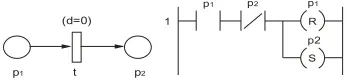
A transition in the EPN model defines the connections between input and output variables in the ladder diagram according to the enabling conditions (1), (2) and firing execution (3). Each input place of a transition in EPN is an enabling condition of that transition (1), therefore input place p1 of the transition t (Fig. 3) is translated
into input in the rung 1 of LD. Each output place of a transition in EPN model is also a condition (2), therefore, output place p2 of the transition t is
translated into a negation of an input in rung 1. This is shown with negated input p2 in rung 1 on Fig. 3. Rung 1 contains also a timer that represents a delay d of the transition t.
t
p1 p2
(d 0)> 1
2
p1 p2
t p1
R p2 S
t d
Fig. 3. Translation of nonzero-time transition from EPN into LD
Firing of a transition in EPN means removing one token from each input place and adding one token to each output place which are connected to the transition with standard connection (3). Token adding and removing is translated in LD as setting of one-bit variable on 1 or 0 respectively. This is presented with a statement in rung 2 in Fig. 3. The variable of timer t (t is set to 1 after the delay d and remains 1 as long as timer is enabled) is a condition in the rung 2 that sets s variable p2 on 1 and p1 on 0.
In this way each nonzero-time transition in EPN has two rungs in LD, the first one for verifying the enabling conditions and the second one for firing execution. Both statements (rungs) could be written in one rung with the timer in the centre, but not all PLC controllers support this kind of programming. Certainly we do this with one rung in the case of zero-time transition which fires instantaneously and does not need a timer. Without a timer both statements are written in one rung as it is shown in Fig. 4. The same applies to
a translation of a transition with n input places and m output places into LD (Figs. 5 and 6).
t
p1 p2
(d=0) 1
p1 p2 p1
R p2 S
Fig. 4. Translation of zero-time transition from EPN into LD
t
pn
p'1 (d 0)> p1
p'm 1
2
p1 p'1
t p1
R
S
pn p'm
pn
R
p'1
p'm
S t d
Fig. 5. Translation of nonzero-time transition with n input places and m output places from
EPN into LD
t
pn
p'1 (d=0) p1
p'm 1
p1 p'1 p1
R
S
pn p'm
pn
R
p'1
p'm
S
Fig. 6. Translation of zero-time transition with n
input places and m output places from EPN into LD
A sequence of statements is also important because it defines the priority of transitions that compete between themselves. The right sequence is significant in case of transitions with at least one common input (Fig. 7) or output place (Fig. 8) since it holds that the statement written in LD before other statements is also executed before others. Therefore, the problem of mutual exclusion still remains on the modelling stage.
pn
p' (d1... n=d 0) p1
tn
t1
p1 p'
2
p1
R
S p' t1
t1
d
pn p'
2n-1
pn
R
S p' tn
tn
d
1
2n
Fig. 7. Translation of n non-zero time transitions with same output place
t1
p'm
p
(d1...dm>0) p'1
tm
p p'1
2
p R
S p'1
t1
t1
d
p p'm
2n-1
p R
S p'm
tm
tm
d 1
2n
Fig. 8. Translation of n non-zero time transitions with same input place
The above rules are true for the standard connections between places and transitions. For the translation of informational connections have the same enabling conditions (1) and (2). The only difference is that the state of the places connected to the transition t with an informational connection stays unchanged after the firing of transition t (Fig. 10).
t1
p1 p2
(d 0)>
1
2
p1 p2
t p2
S
t d
Fig. 9. Translation of nonzero-time transition with negated input place
The above described rules for the standard connections between places and transitions. For
the translation of informational connections hold the same enabling conditions (1) and (2). The only difference is that the state of the places connected to the transition t with informational connection stays unchanged after firing of transition t (Fig. 10).
t1
p1 p2
(d 0)>
1
2
p1 p2
t p2
S
t d
Fig. 10. Translation of nonzero-time transition with informational connection of input place
3 TEST CASE
The modelling with PN extensions, translation of EPN model into LD programme and simulation with PLC were initially tested on a control example of a electropneumatic system composed of a double acting pneumatic cylinder
A with two end-switches (a0 in a1), 4/2-way valve
KA and programmable logical controller with start and stop buttons (Fig. 11).
Fig. 11. Electro-pneumatic system and state diagram for extend and retract stroke
3.1 Formal Description of Operation
The diagram in Fig. 11 describes the forward and backward movements of the cylinder
A and the states of the end switches. When switch
a0 or a1is on, the cylinder (actually a piston-rod
of the cylinder) is in retracted (home position) and extended position (out position) respectively. If both switches are off, the cylinder is in movement. Retracting and extension strokes are controlled by signals S2 and S1 that switch the
pressure or exhausted. For the extension stroke (fort movement) the air pipe P1 needs to be under
pressure and P2 exhausted, and in the other way
for the retraction stroke (back movement).
The time scale of a stoke shows that the stroke has two parts: the switching part and the stroke itself. The switching part starts when the signal for a stroke is given, and last to the moment when the piston starts moving. The stroke itself starts at the beginning of the motion of the piston and lasts until the piston stops in new position. In Fig. 11 the time for switching part is denoted with tv1 and tv2, and the duration of
the stroke with th1 and th2 for fort and back
movement respectively. During the switching time tv1 and tv2end switches are turned on (signals a0 and a1 are 1).
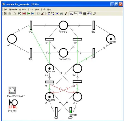
3.2 EPN Model of Double Acting Pneumatic Cylinder
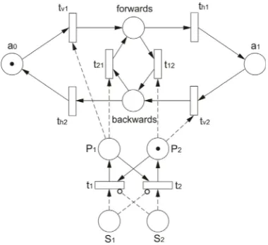
On the basis of the formal description of operation of double acting pneumatic cylinder and 4/2-way valve an EPN model was built (Fig. 12). The places in the graph represent states of the cylinder (a0, a1, fort, back), the valve (P1 and P2)
and of the input signals (S1 in S2). Transitions (t1, t2, tv1, th1, tv2, th2, t12 in t21) represent actions or
events that change the state of the system. Regarding the control signals S1 and S2,
the 4/2-way valve is in one of two states denoted by P1 or P2. States P1 and P2 indicate which
output port of the valve is under pressure or exhausted (port 2 or 4). A regular operation of double acting pneumatic valve consistently appoints that just one of the air ports should be under pressure and the other one has to be exhausted. Operation of the valve is modelled by transitions t1 and t2, which according to the state
of the signals S1 and S2 remove and add a token
from and to the place P1 or P2. If the signal is on
both solenoids, the valve does not change the state and so the negations of the signals S1 in S2
are added to the transitions t1 and t2. The signals S1 and S2 do not change the state when the valve
is switching, so the connections from places S1
and S2 to the transitions t1 and t2 are informational
and represented in the graph by a dashed line (Fig. 12).
The states of the cylinder are modelled by the places a0, forward, a1 and backward. The
transitions between places tv1, th1, tv2 and th2
model switching part of forward and backward movement, and forward and backward strokes. The transitions t12 and t21 model a change of a
stroke direction during the piston movement. States of the places P1 and P2 are changed just by
transitions t1 and t2, so the connections from P1
and P2 to transitions tv1, tv2, t12 are t21 are
informational.
Fig. 12. EPN graph of a model of a double acting pneumatic cylinder controlled by 4/2-way valve
3.3 Test of the EPN Model
With analytical methods using matrix equations or with the reachability tree the EPN model can be analyzed against boundedness, reachability and liveness. The duration of nonzero-time transitions has no influence on these characteristic. However, due to mutual exclusion and concurrency, the delays of nonzero-time transitions have a significant influence on a firing sequence of these transitions and, therefore, also on reaching the required state. Thus, the verification of the model that will prove if the model corresponds to the operation of real system is needed. This can be accomplished by executing (playing) the graph i.e. firing the enabled transitions and changing the marking of the places (moving tokens between places). The graph can be played manually (that is also for the simplest model very time consuming) or by computer simulation.
or just support modelling and playing the PN graph. But the elaborated extensions of a basic theory of Petri net are distinctive and require dedicated modelling and simulation programme. The alternatives were to build a new simulation programme for elaborated EPN or to build EPN building blocks with embedded firing logic within an existing simulation programme. The second alternative was more practical and so the discrete
simulation programme Tecnomatix Plant
Simulation has been chosen for the development platform.
On the basis of standard building blocks of
Tecnomatix Plant Simulation and the ability of programming their behaviour, new customized building blocks for places, transitions and connections were developed. There is one type of building blocks for places, one type for transitions and three types for connections: standard connection (black line), informational connection (green line) and negated connection (red line). With these building blocks an accurate and consistent EPN model can be built and the execution of the graph according to the enabling and firing rules of elaborated EPN can be performed.
A simulation of the EPN model within a programme for discrete simulation enables the delays of transitions to be arbitrarily altered during the simulation. This is especially important for the verification of the model in the case of switching the direction during the stroke. The calculation of the time of transition th1 and th2
that depends on the distance of the piston from the end position and its velocity can be easily added to the behaviour of the building block of these two transitions.
For the analysis of the EPN model of the double acting pneumatic cylinder and the 4/2-way valve two additional transitions fwd and bwd were placed into the model (Fig. 13). The transitions
fwd and bwd actually randomly and automatically change the states of the signals S1 and S2, and so
enable a continual execution of the model for the analysis.
During the test the model was never blocked and the required state was always reached. The result of this analysis proves that the EPN model is an accurate model of the operation of the observed system.
Fig. 13. Analysis of the EPN model within the programme for discrete simulation
3.4 Translation of EPN Model into Ladder Diagram
The EPN model of double acting pneumatic cylinder with the 4/2-way valve (Fig. 12. ) was translated into ladder diagram (Fig. 14) according to the elaborated translation rules. Each transition with instantaneous firing (t1, t2, t12 and
t21) is translated in the ladder diagram into one
rung (rungs 2, 3, 12 and 13 on Fig. 14) and nonzero-time transitions (tv1, th1, tv2 in th2) into
two rungs (rungs form 4 to 11 on Fig. 14). To the transitions t12 and t21 the function that calculates
the delay (duration) of the transitions th1, and th2
(last line in rungs 12 and 3 on Fig.14) was added. The function calculates the duration by subtracting the remaining time of the previous stroke from the whole stroke in a new direction and multiply that by the ratio between the duration of the previous stroke and the duration of the stoke in new direction. The statement in the first rung of ladder diagram sets the initial state of the model according to the initial marking of the places M0 and is executed in the first cycle after
the PLC programme is started.
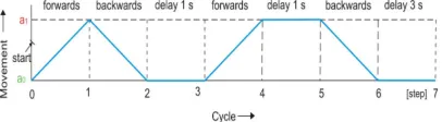
3.5 Testing Example
translated ladder diagram of the EPN model of the cylinder-valve system (Fig. 14) and the control part with the test sequence (Fig. 15). The control part of the PLC programme was also modelled with the EPN and translated into LD. The EPN model of the control algorithm for the test sequence was added to the EPN model of the tested system and verified within the programme for discrete simulation (Fig. 16).
12 R
S
npr_fwd P2 npr_fwd
nz _bwdj tv2
dv2
8
a1 P2
nzj_bwd
9 R
S
tv2 a1
th2
dh2
10 nzj_ wdb
a0
11 R
S
th2 n _ wdzj b
3 R S S1 tv1 dv1
S2 P1 P2 P2
P1
R S S1
S2 P2 P1
P2
P1
4
a0 P1
npr_fwd
5 R
S
tv1 a0
th1 dh1 6 npr_fwd a1 7 R S
th1 npr_fwd
2
= dh1
13 R
S
nzj_bwd P1 n _ wdzj b
npr f_ wd
= dh2
(t )2
(t )1
(t )v1
(t )v1
(t )h1
(t )h1
(t )v2
(t )21
(t )12
(t )h2
(t )h2
(t )v1
P2
1
S M0
(M0)
S
S a0
M0
Fig. 14. Simulation part of PLC programme
Fig. 15. Test sequence of strokes
The algorithm for the control sequence uses the step function methodology. Each step in the sequence has a corresponding transition and place in the EPN model. If the conditions (marking of the places) for the next step are fulfilled than the corresponding transition fires and marks the next step place. Input places to these transitions (from step_1 to step_7 in the EPN model in Fig. 16) are places that represent step succession of control algorithm (step1 to
step7) and the places that define the state of the cylinder-valve system (a0 and a1). Output places
of these transitions are places for the succession of control algorithm and places that represent control signals to the valve (S1 and S2). All
connections from and to the control transitions except from the places a0 and a1 (sensors) are
standard connections. Connections from the places a0 and a1 are informational connections.
Place start represents state of the start button and is set or reset manually. In real PLC this corresponds to the input variable of the start button.
Fig. 16. Testing the simulation and control part of the PLC programme within a programme for
discrete simulation
After the validation of the control part of the PLC programme with EPN model in the programme for discrete simulation (Fig. 16), also the EPN model of the control part of the PLC programme was translated into the ladder diagram (Fig. 17). T1 R S S1 5 R S step2 step3 S2 R S a0 T1 1 s
step7 S2
S1
4
step2 a0
2 start R S step7 step1 R S a1
step1 S1
S2 3 R S step1 step2 T3 3 s 10
step2 a0
T3 R S 11 step6 step7 S S S2 step7 M0 1
Fig. 17. Ladder diagram of the control part of the PLC programme
represent instantaneous transitions that switch the next step in the control sequence.
3.6 Test of the Simulation With the PLC Emulation
The simulation with PLC emulation was tested on two PLC programming platforms ( CX-Programmer with CX-Simulator from Omron and
STEP 7 with 7S PLCSIM from Siemens) that comprehend also simulation i.e. emulation of PLC on a PC computer. The control (Fig. 17) and simulation part (Fig. 14) of the PLC programme were put into the PLC programme in the usual way of PLC programming. The PLC programme can be written for virtual or real PLC. In both cases the input and output variables have the same format.
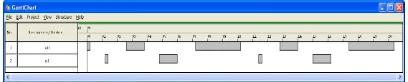
After the PLC programme had been transferred to the emulated PLC (in the same way the PLC programme is transferred to the real PLC), the PLC programme ran and simulated the operation of the controlled system. The simulation of the system operation was observed using a graphical presentation of PLC programme execution which programmers usually use in their
everyday work. A tracking function (
CX-Simulator) that captures and presents the states of the variables in time chart (Fig. 18) was also very useful. This is very convenient for detecting and eliminating the errors in the PLC programme.
Fig. 18. Time chart of the states of the end switches a0 and a1 tracked during the simulation
with PLC emulation (CX-Simulator)
Fig. 19. Time chart of the states of the end switches a0 and a1 tracked during the simulation
of the EPN model in Tecnomatix Plant Simulation
Visual comparison of graphical presentation of PLC execution showed that the control and simulation part of the PLC
programme as well as the concept of simulation with real or emulated PLC fulfilled the expectations. A confirmation for that is also the comparison of the time charts of states a0 and a1
obtained by the simulation of EPN model in
Tecnomatix Plant Simulation (Fig. 19) and by the PLC emulation with CX-Simulator (Fig. 18).
4 APPLICATION CASE AND THE PERSPECTIVES
The elaborated method was used for modelling of an automated assembly station which was used in practical lectures for learning about the operation and control of automated components, and programming of PLCs. The assembly station consists of electro-mechanic dividing table, 2-axes pneumatic manipulator with a gripper, two screw drivers and control device [7]. All axes and drives of all the components in the assembly station can be regarded as discrete, stand-alone and two-position (initial and end position) systems, so their operation can be modelled in the same way as the operation of the cylinder-valve system on Fig. 11. Each of the axes and drives is also autonomous, so the EPN model of the assembly station consists of 8 sub-models (2 for 2-axes manipulator, one for gripper, 2 for each screw drive and one for dividing table).
Experiences with simulation based on emulated PLC in a practical course have shown that this is a very useful learning tool for the curriculum in the field of assembly and handling automation. There are two particularly important benefits to mention:
- The operation and programming of the PLC
can be described and explained without using a real system. This can be done in a lecture room or in a computer room where each student can programme and test the PLC programme on the PC computer.
- Students can use the PLC programming tool
with PLC emulation on PC computers at home and can in this way do more exercises and complete the assigned practical work. In addition, they can test the already verified PLC programme on real PLC in laboratory or even with remote access from home in a so called remote laboratory [7].
industrial PLC programming tools, SCADA based graphical user interface and LabVIEW remote panel for remote laboratory is the direction of modern tools for learning and training of automation and mechatronics.
5 CONCLUSION
A control of modern automated machines and devices in process and bulk production industry is nowadays generally accomplished by programmable logical controllers (PLC). Knowledge about PLC programming is the basis for practical work of mechanical, electrical and mechatronic engineers along the entire lifecycle of machines or plants – from engineering to operation, maintenance and modernization. The modelling and simulation can significantly help the teaching and learning of PLC programming, training of the operators and maintaining personal, developing automated systems and diagnosis of the systems’ operation.
The challenge for the presented work was to develop a way of building a model and running a simulation by the tools commonly used in the industrial environment. The basic idea was to use the PLC programming tool for modelling a discrete mechatronic system and simulate its operation on industrial PLC or on emulation of PLC on the PC computer. The main issue was to build an accurate and valid simulation model with a tool designed for writing the control programmes.
For the realization of the idea the extensions of the basic Petri net theory (EPN) were elaborated, which enabled a building of an accurate model of a discrete system including a related control programme. Unified, direct translation of the EPN model into the ladder diagram was developed, which enabled the use of the EPN model for simulation on PLC or emulation of PLC. Furthermore, the building blocks of the EPN model were developed within the programme for discrete simulation, which enabled the building and verification of an EPN model within the programme for discrete simulation.
The elaborated extensions and developed tools were primarily tested on a case of operation of double acting pneumatic cylinder with a 4/2-way valve. The results of the verification of the EPN model with discrete simulation and the
simulation of the cylinder-valve system on the emulated PLC show that the elaborated extensions of Petri net and the developed translation of EPN model into the ladder diagram completely fulfil the settled requirements and can be used in practice. The usability of the basic idea was verified during the practical course on assembly automation. The simulation on emulated PLC was used for explaining the basics of PLC programming and for developing the control programme for a real automated assembly station. The results show that the method is applicable for teaching and learning of PLC programming as well as for advanced developing and testing of PLC programmes. The future of the method in industry is in the field of training and introducing of operators and maintainers before system installation, and for model based diagnostic of automated system.
6 REFERENCES
[1] Frey, G., Lothar, L. Formal methods in PLC
programming, Proceedings of the IEEE
Conference on Systems Man and Cybernetics SMC 2000, Nashville, Oct. 8 - 11, 2000. [2] Bogdan, S., Smolić-Ročak, N., Kovačić, Z.
A testbed for analysis of PLC-controlled manufacturing systems. Proceedings of the 10th Mediterranean Conference on Control and Automation - MED2002, Lisbon, Portugal, July, 9 - 12, 2002.
[3] Polič, A., Jezernik, K. Closed-loop matrix based model of discrete event systems for
machine logic control design. IEEE
transactions on industrial informatics, February 2005, vol. 1, no. 1, p. 39-46. [4] Iversen, W. Digital manufacturing: Chasing
the vision, AutomationWorld, April 2008. [5] Waurzyniak, P. (2007) Enter the virtual
world: A new generation of digital manufacturing software tools offer manufacturers a better virtual factory,
Manufacturing Engineering, vol. 139, no. 4. [6] Perme, T., Noe, D. A "Low-cost" solution of
virtual manufacturing systems. Preprints of the 13th world congress International
[7] Perme, T., Drev, V., Noe, D. Remote assembly system for education. International Symposium on Remote Engineering and Virtual Instrumentation 2006, June, 29 - 30, 2006, Maribor.
[8] Perme, T., Noe, D. E-training remote
assembly systems. IFAC Multitrack
Conference on Advanced Control Strategies for Social and Economic Systems, Vienna, September, 2 - 4, 2004.
[9] Kopacek, P., Kronreif, G., Perme, T. Simulation within CAD-environment. In: Brandimarte, P. (editor), Villa, A. (editor).
Modeling manufacturing systems: from aggregate planning to real-time control.
Berlin [etc.]: Springer, 1999, p. 116–137. [10] Perme, T., Noe, D. Erweiterte Petrinetze zur
intelligenten Planung von Produktionssystemen. Int. j. autom. Austria,
2002, vol. 10, no. 2, p. 111-124.
[11] Perme, T., Noe, D. Simulation mit
Erweiterten Petri-Netzen zur Planung von Montagesystemen. Int. j. autom. Austria, 2004, vol. 12, no. 1, p. 1-16.
[12] Kunc, M. A., Kunc, V., Diaci, J., Karba, R. (2008), Modelling and analysis of a combined electronic and micro-mechanical system, Strojniški vestnik - Journal of Mechanical Engineering, vol. 54, no. 7-8, p. 539-546.
[13] Matta, A., Semeraro, Q., (editors) Design of Advanced manufacturing Systems: Models for Cpacity Planing in Advanced Manufacturing Systems, Springer 2005.
[14] Mušič, G, Gradišar, D. Matko, D. IEC
61131-3 Compliant Control Code Generation from Discrete Event Models,
Proceedings of the 13th Mediterranean
Conference on Control and Automation, Limassol, June, 27 - 29, 2005, p. 346 – 351. [15] Peng, S., S., Zhou, M., C. Ladder Diagram
and Petri-Net based Discrete-Event Control
Design Methods, IEEE Transactions on
System, Man, and Cybernetics, vol. 34, no. 4, November 2004.
[16] Peng, S., Zhou, M.C. Sensor-based Petri net modeling for PLC stage programming of discrete-event control design, Proceedings of the 2002 IEEE International Conference on Robotics and Automation, Washington DC, May 2002.
[17] Latha, K., Umamaheswari, B. Supervisory control of an automated system with ladde logic programming and analysis using Petri nets. In: Proceedings of the second IEEE International Conference on Systems, Man and Cybernetics (SMC'02), October, 6 - 9, 2002, Hammamet, vol. 3, IEEE Computer Society Press, October 2002.
[18] Peterson L.J. 1981, Petri net theory and modeling of systems. Prentice-Hall International.
[19] Reisig, W. Petrinetze; Eine Einführung, Springer-Verlag, 1991.
[20] Murata, T. (1989), Petri nets: properties, analysis and applications, Proceedings of the IEEE, vol. 77, no. 4, p. 541-580.