0 INTRODUCTION
Robustness is a key factor of product design under uncertainty from material properties, manufacturing operations and practical environment. Actually, from designer’s brain to users’ hands, the product must pass through many stages of its life cycle. The variability generated at each stage obviously has an influence on the performances of the product. It can be the cause of the designed product not fully meeting the requirements of the customers and users.
Each part of making up the product is manufactured from raw material in the manufacturing stage using processes such as forging, cutting or grinding. Geometrical deviations are generated and accumulated on each part over the successive set-up of the manufacturing process due to inherent imperfections of raw material, tooling and machine. Then, the parts with deviations are assembled at the assembly stage. The deviations of the surfaces of the assembled parts generated at manufacturing stage affect the assemblability and the final geometry of the product. The geometry of the final product is, therefore, different from the nominal one at the end of these two production stages. On the other hand, the current product modelling technology is not capable of taking into account these deviations. Most of the simulations performed to predict the behaviour and the performance of a product (kinematics, dynamics, aerodynamics, etc.) are based on the nominal model of the product. Since this model cannot deal with geometrical deviations generated throughout the product life cycle, the variation of product behaviour and performance cannot be predicted. Thus, the “real” performance of the product, which is different from the designed one (nominal performance), cannot be
verified. The risk is then that the designed product fails to fully meet customers’ and users’ requirements in which situation, the product-process design has to be considered as not good or at least not robust.
Many methods and tools are proposed in the academic research in order to manage the effects of geometrical variability on a product design. However, only mentioned manufacturing or assembly stage of the product life cycle is mentioned. In [1], the authors addressed the impact of the manufacturing errors on the performance of the product. They defined the Manufacturing Variation Pattern (MVP) to represent the manufacturing characteristics and investigated its effects on the performance of the product. In [2], the authors presented the theory that offers an analytical and geometrical description of the performance sensitivity distribution of a product in the variation space. The theory can be applied to find the robust design less sensitive to the dimensional variation due to manufacturing errors or product wear. The authors in [3] proposed a new Probabilistic Sensitivity Analysis (PSA) approach for the design under uncertainty based on the concept of relative entropy. This approach allows providing the valuable information about the impact of the design variables on the performance of the product and the whole range or a partial range of the performance distribution. In [4], the authors proposed a statistical approach in order to evaluate the impact of geometrical variations on the angular rotational velocity between two bevel gears. The Monte-Carlo simulation method is used to consider the geometrical behaviour simulation and tooth contact analysis. The authors in [5] proposed a methodology for quantifying the kinematic position errors due to manufacturing and assembly tolerances.
A Method to Determine the Impact of Geometrical Deviations on
Product Performance
Vignat, F. – Nguyen, D.S. – Brissaud, D. Frédéric Vignat1 – Dinh Son Nguyen2 – Daniel Brissaud1
1 University of Grenoble, G-SCOP Laboratory, France
2 Danang University of Technology, The University of Danang, Vietnam
Robustness is the key to successful product design when many variation sources exist throughout the product lifecycle. Variations are of many sources such as material defects, machining errors, and use conditions of the product. Most of product performance simulations are traditionally carried out using the numerical model created in the CAD system. This model only represents the nominal information about the product. Thus, it is difficult to take these variations into account in product performance prediction. A method is proposed in this paper to allow integrating the effect of these variation sources into the product performance simulation. This method is based on a random design of experiment method. As a result, an image of the “real” performance of the product is determined.
Based on this method, a kinematic amplitude variation for bodies’ position is calculated.
In [6], the authors proposed to integrate material and manufacturing process uncertainties in the design in order to consider their impacts on the performance of the product. They developed a procedure for uncertainty propagation from the material random field to the end product performance based on the product finite-element mesh. In mechanical assembly, there are several statistical approaches to determine the effect of geometrical deviation introduced in [7]. The authors in [8] proposed a tolerancing model, called Proportioned Assembly Clearance Volume (PACV), based on the Small Displacements Torsor (SDT) concept. This model aims to determine the effect of geometrical deviation of surfaces on an assembly. In [9], the authors proposed a new calculation method to analyse the geometrical deviations stack-up in the assembly line (parallel and serial assembly line) on the product designed. The authors in [10] introduced a model of geometrical product specifications for product life cycle. This model allows the communication of geometrical information which can come from design, manufacturing or inspection.
These studies examine the impact of geometrical variations in manufacturing or assembly stage on the designed product. However, the effects of the variation sources during the product life cycle on the performance of the product are not mentioned. Especially, the mathematical relationship between the performance of the product and the parameters of variation sources is unknown. In many cases, this relationship is not established and numerical resolutions using tools such as finite elements used to determine the performance for one specific set of values of the product parameters. One numerical solution thus determines one point on the response surface of the relationship between the performance of the product and the product parameters. In order to establish an approximation of the required relationship, this paper proposes to use a set of numerical solution combined with a design of experiment.
In order to study the effect of geometrical variability on product performance, there are important issues that have to be considered:
• How to establish the relationship between the
performance and the geometrical deviations of the product?
• How to manage the causes and consequences of
these deviations at design stage?
This paper proposes, as an answer to the first question, a method that allows establishing the relationship between performance and geometrical
deviations. The geometrical deviations generated and accumulated are modelled by the geometrical deviation model presented in [11] and reminded at the beginning of Section 3. A partial answer to the second question has been proposed in [12] for identification and classification of the influence of the deviation parameters.
1 INCLUDING GEOMETRICAL DEVIATIONS IN PRODUCT PERFORMANCE SIMULATION
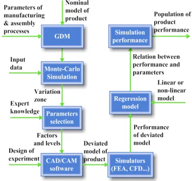
There are many kinds of disturbances, during the product lifecycle, which may influence product quality and functionality [13]. In order to investigate their effect on the product performance, a method that allows taking them into account in the product performance simulation is proposed in this section. The overview of the proposed method is shown in Fig. 1.
Fig. 1. Performance simulation of the product with geometrical deviations
This relationship is used to generate an image of the product population performance from the “real” product population with geometrical deviations.
1.1 Geometrical Deviation Model
As presented above, the nominal model of a product created in CAD/CAM systems can only represent nominal product information and cannot handle geometrical deviations generated and accumulated during the product life cycle and especially at manufacturing and assembly stage. The GDM, as presented in [11], can model them based on small displacement torsor. A small displacement torsor T at a point O in the Cartesian coordinate system (O, X, Y, Z) is described by rotational vector R and translational vector D as shown in equation as follows:
T =
{
R D,}
{O X Y Z, , , }.A surface deviation torsor is a small displacement torsor describing the deviation between an associated surface and a nominal surface. The associated surface is an ideal surface associated with the real surface using a minimum distance criterion such as the least square. For example, the deviation torsor of the associated plane relative to its nominal position is described by the SDT TSurface at a point O in the local
coordinate system (O, X, Y, Z), as shown in equation
as follows:
T
rx ry tz
Surface
O X Y Z
=
{ }
0 0 0
, , ,
,
where rx, ry are rotational and tz translational
components regarding X, Y, Z axis, respectively. The
plan, in this case, has three degrees of freedom, so three positioning deviations of the plan are invariant (i.e. cannot be measured due to the surface class) relative to their nominal position and their values are arbitrarily fixed. Thus, the 0 value is chosen in order to hide the notion of invariance.
The GDM model, for the manufacturing stage, is based on the model of the manufactured part (MMP) proposed by [14]. The geometrical deviations generated by a manufacturing process are considered to be the result of two independent phenomena: positioning and machining, and are accumulated over the successive set-ups. The manufactured deviations of the part surfaces are expressed relative to their nominal position by a SDT TP Pi
j i
, .
TP Pi TSj P TSj P
j
i i
j i
, = − , + , , (1)
where TSj P, i models the positioning deviation of
workpiece in set-up Sj. This deviation is a function of the MMP surfaces deviation generated by the previous set-ups, the part-holder surfaces deviations and the links part-holder/part surfaces.
TSj P
j i
, models the deviation of the machined
surface j realised in set-up Sj. This deviation is
expressed relatively to the nominal machine. This torsor merges deviations of the surface swept by the tool and cutting local deformations.
A product is made up of parts assembled by the way of connections. Each part has already passed through the manufacturing stage where geometrical deviations were generated. Then, the product passes through assembly stage of its life cycle. The assembly stage brings its share of deviations to the product. The GDM for the assembly stage is based on the model of the assembled part (MAP). The positioning deviations of each part relative to its nominal position in the global coordinate system of the product are modelled by a SDT TP P, i.
TP Pi TP Pk TP Pk TP P TP P
nk nk mi i mi
, = , + , + , + , , (2)
where TP P
nk, mi is the link torsor between surface m of
MMP i (part i) and surface n of MMP k (part k). TP P, k
is the positioning deviation torsor of part k, it models the positioning deviation of the part k (a subassembled part coming from the previous set-up of the assembly process) relative to their nominal position in the global frame of the product.
The GDM establishes the mathematical relation between the deviation sources from the manufacturing and assembly stage and product surfaces deviations. A Monte-Carlo simulation method is then used to create a set of M products with geometrical deviations
(M generally chosen between 10,000 and 1 million).
As a result, the product designers can be aware of the distribution of the product surfaces deviation [15].
1.2 Design of Experiment
as finite element, computing fluid dynamics, etc. For a complex product system, it is, however, difficult
to create M models of the product with geometrical
deviations and to calculate the performance of M
products because performance simulations can be time consuming (several hours for one simulation). Thus, it is not possible to perform simulation for the M
products. In order to overcome this limitation, a DOE approach is proposed to determine an approximated mathematical relationship between the performance of the product and the product parameters deviation. Then, it is possible to determine the performance of the M products by using this relationship.
Considering that each simulation is CPU time intensive, it is necessary to limit the number of simulations to be performed. The number of simulations increases with the number of factors taken into account for the design of experiment. It is thus necessary to limit this number of factors. These factors are geometrical deviation parameters and are defined based on expert knowledge. These key parameters are measured on the virtual product and are functions of the elementary deviation parameters. The value of these factors can be calculated by using the result of
Monte-Carlo simulation of the M products.
The design of the experiment requires a defining level for these factors. The number of levels for these factors is chosen based on a compromise between the desired precision and the calculation time. The values of the factor levels are then calculated according to the factor range of variation. Depending on the number of factors n, the number of levels k and the
chosen strategy, the number of deviated products N
are determined. The corresponding N values of the
n factors are gathered in a matrix P named design
matrix, as shown in Eq. 3.
P
p p p
p p p
p p p
n n
N N nN
=
11 21 1
12 22 2
1 2
... ... ... ... ... ...
...
. (3)
Next, simulation tools as FEA, CFD, etc., are
used to calculate the performance of the N products.
A set of N deviated models of the product has to be
created in the CAD system. Each deviated model of the product j is modelled according to the value pij of the factors. The performance of each product is then calculated and finally, the performance of the
N products is gathered in a vector R called response vector as expressed in Eq. (4).
R r r
rN
=
1
2
... . (4)
The relationship between the performance of the product and the selected factors {p1, p2, p3, ..., pn}
is established using a regression model and can be expressed by Eq. (5).
Performance = f (p1, p2, p3, ..., pn). (5) For example, the linear least square fit model [16] can be used to establish the relationship in the case of n
factors and 2 levels. From the result of 2n simulations, the relationship is expressed by a function as given in Eq. (6).
f = ⋅ +β� p ε, (6)
where ε is the residual vector, p = {p1, p2, p3, ..., pn}T is a vector gathering the n factors, β� is a coefficient vector of the model. It is calculated by Eq. (7).
β
� =(P PT⋅ )−1⋅P RT⋅ , (7)
where R = {r1, r2, r3, ..., rN}T is a response vector including N simulation responses.
The performance for the population of M products is then calculated by replacing the value of the selected factors {p1, p2, p3, ..., pn} with the collected data from the Monte-Carlo simulation into Eq. (5).
1.2.1 Factorial Design
As mentioned before, the number of simulations to be performed depends on the number of factors, the number of levels and the chosen strategies. In this paper, three strategies are proposed and can be chosen depending on the required precision, expert knowledge, the number of factors and calculation time. Two strategies, full factorial and Taguchi design, are commonly used while the last one, while random design is original.
virtual product and are functions of the elementary deviation parameters. The variation range of these factors can be determined based on the M results from the Monte-Carlo simulation. The value assigned to the levels of these factors is determined according to these ranges of variation. The kn values of the n
parameters are then gathered in the design matrix P.
An extended description of the use of full factorial design of experiment has been presented in [18]. With full factorial design of the experiment, the number of numerical simulations increases dramatically with the numbers of selected factors and levels. For example,
23=8 simulations are necessary in the case of three
factors and two levels (see Fig. 2). It is then necessary to find some alternatives to this method.
Fig. 2. Full factorial design with three factors, two levels
1.2.2 Taguchi Design
One alternative method is Taguchi’s orthogonal arrays. This method has been designed in order to reduce the number of simulations to be performed.
Table 1. Table of Taguchi design
Number of levels (
k
) Number of factors (n)
2 3 4 5 6 7 8 9 10 11 12
2 L4 L4 L8 L8 L8 L8 L12 L12 L12 L12 L16
3 L9 L9 L9 L18 L18 L18 L18 L27 L27 L27 L27
4 L16 L16 L16 L16 L32 L32 L32 L32 L32 5 L25 L25 L25 L25 L25 L50 L50 L50 L50 L50 L50
Taguchi’s orthogonal arrays are highly fractional orthogonal designs proposed by Taguchi. They are used to estimate the main effects with only a few experiments. This approach is also suitable to apply for certain mixed level experiments where the factors included do not have the same number of levels.
The number of factors is selected from expert knowledge in order to eliminate the factors that have few effects on the performance of the product. The value associated with the levels of each factor is also
defined from the results of the geometrical deviation Monte-Carlo simulation. Then, the number of experimental to run is selected based on the Taguchi’s
orthogonal arrays, as shown in Table 1.In the case of
n factors and k levels, there are Ln experimental runs that must be realized according to Taguchi table. For example, it is necessary to create 4 deviated models of the product for the performance simulation in the case of 3 factors and 2 levels. The design matrix P in this case is different from the one from factorial design. It is defined according to Taguchi table for each factor and level, as given in Eq. (8).
P= + + − −
+ − + −
− + + −
1 1 1 1
1 1 1 1
1 1 1 1
. (8)
An extended description of the use of Taguchi’s orthogonal arrays has been presented in [17] and [18].
1.2.3 Random Design
In case of increasing complexity alongside with the number of factors, the number of necessary simulations to determine the relationship between performance and deviations can become too large and thus time consuming even when using Taguchi design. Moreover, the use of expert knowledge to determine key factors filters the deviation sources and can reach the list of some influential factors. Factorial design and Taguchi’s orthogonal arrays are not effective in this case. Thus, a random design of the experiment method is proposed in order to address these issues. All product geometrical deviations parameters, called factors {pi} (i = 1, ..., n)that have small effects on the performance of the product are taken into account.
The random design approach is realized in four steps (see Fig. 3):
Fig. 3. Algorithm diagram of random design
• Step 1. Draw randomly a product with geometrical
A kth product with geometrical deviations is randomly drawn in a set of M products collected from results of geometrical deviation simulation. The value of each factor
{ }
p ii ( 1,.., )= n is calculated based on the drawnproduct deviation parameters values. The set of values of the factors {pi} (i = 1, ..., n) is added into the kth row of the design matrix P.
• Step 2. Create the deviated CAD model.
The deviated model of kth product will be created
in the CAD software corresponding to the value
of each geometrical deviation parameters {pi}
(i = 1, ..., n).
• Step 3. Simulate the performance of the product.
The deviated model created in Step 2 is used to simulate the performance of the product in order to determine the performance of the representative product. The result is appended into the response vector R.
• Step 4. Eliminate the drawn product in the set of
M products.
Repeat from Step 1 until the number of the drawn product reach the desired number N.
The main limitation of this method is the
definition of the number N of simulations to be
run. The number N of products drawn is defined
considering the balance between the required precision and the expected calculation time. However, the problem is similar to that of every stochastic method were the size of the sample is a key parameter.
2 A CASE STUDY
The DOE method to integrate geometrical deviation in product performance simulation has already been applied to the complex example of a centrifugal pump [19]. In this application Factorial and Taguchi strategies have been used. In the present paper, the three strategies are applied to the same case for the purpose of comparison and evaluation. Thus, a simple example, a harmonic oscillator, is proposed in order to save calculation time (less than 1 ms per simulation) and to compare the three strategies to the analytical result which is known in the present case.
2.1 A harmonic Oscillator
The harmonic oscillator system includes a spring and a mass (see Fig. 4). The performance considered in this case is the natural frequency of the oscillator. The natural frequency of the oscillator is expressed by Eq. (9).
f k
m
= 1 ⋅
2π , (9)
where m is the mass of the load which depends on its
density ρ and its volume. Thus, the load mass deviation depends on the geometrical deviations of the load surfaces. For example, the deviations of the cylinder radius and of the position of the two boundary planes (rotation and translation) affect the mass m. The mass is calculated by Eq. (10).
m = ρ · V, (10)
k is the spring constant or spring stiffness and it is calculated by Eq. (11).
k Gd
nD
= 43
8 , (11)
G= E
+
2 1( υ), (12)
where E is Young’s modulus, d spring wire diameter,
D spring mean diameter, n number of active windings
and n a Poisson ratio.
From Eqs. (10) to (12), the variation of the frequency is obviously affected by geometrical deviations of the surfaces of the mass and the spring. Deviation torsor parameters of each surface, given in Table 2, influence the natural frequency of the mass-spring system.
Table 2. Geometrical deviation paramaters
Component Geometry Deviation
parameters Description
Mass
Plan 1 Rx1, Ry1, Tz1 Parameters of deviation torsor of plan P1
Cylinder 2
Rx2, Ry2 Tx2, Ty2 Parameters of deviation torsor of cylinder C2
dr Radius deviation
of cylinder C2
Plan 3 Rx3, Ry3, Tz3 Parameters of deviation torsor of plan P3
Spring Spire ∆, δ Deviation of spring outer and wire diameter
The geometrical deviations of each surface of the mass-spring system are modeled by a GDM as presented in Section 1 and the Monte-Carlo simulation method is then used to give an image of the “real” production of the mass-spring systems.
For example, the distributions of the cylinder’s
deviations of 100,000 virtually produced loads are
deviation (Tx2, Ty2) of cylinder C2 relative to X and
Y axis are shown in Figs. 6a and b. These deviations
can be included in the volume V calculation and by
using Eq. (10) the mass deviation can be determined as shown in Fig. 6c.
Fig. 4. Mass-spring system
From the expert knowledge presented above, the relationship between the frequency of the spring system and its geometrical deviations can be determined and expressed by Eq. (13).
f G d
n D h R h dr R
R h Tz R h Tz
= +
+ − + + +
+ + + +
1
4 2 2
4
3 2 2
2
1 2
π
δ
ρ π π
π π
( )
( ) ( )
( ) (
∆
33)
,
(13)
where h, R and r are respectively nominal height,
radius and density of cylinder C2 of the load.
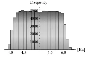
In fact, the frequency simulation of this system can be realized using the Eq. (13) directly. A population of 100,000 frequencies is generated from the results of the Monte-Carlo simulation mentioned in [15]. The histogram of the 100,000 frequencies calculated is shown in Fig. 6. An approximated relationship between the frequency and the geometrical deviation parameters is then established
Fig. 5. Monte-Carlo simulation results
using a linear regression model with the 100,000 frequencies data. This equation given in Eq. (14) is the most precise possible linear regression approximation. It will be used for the purpose of comparison with the other approximations.
Fig. 6. The distribution of frequency f = 4.79048 ‒ 0.0547296Tz1 ‒ 0.155346dr ‒
‒ 0.0545993Tz3 + 2.48972δ ‒ 0.149673∆. (14)
The three other DOE strategies will then be applied to this simple example to compare accuracy among them. The results will also be compared to this first approach that will be used as a benchmark.
2.1.1 Factorial Design
From expert knowledge as given in Eq. (13), geometrical deviation parameters of the load and the spring that have a strong influence on the natural frequency of the oscillator are defined as factors. These factors are selected as follows for the factorial design study:
• Tz1, Tz3: translational deviation of the two planes
of the load P1, P3,
• D,d: deviation of the spring mean and wire
diameter,
The number of levels for the five factors is chosen as two and the number of runs is thus 32. The levels for the factors are calculated from the results of the Monte-Carlo simulation. The low and high levels are respectively selected at ‒3s and +3s of each factor distribution. The relationship between the frequency and selected factors is established by using a linear regression model from the 32 runs results. This function is expressed by Eq. (15).
f = 4.82605 ‒ 0.0560401Tz1‒ 0.16062dr ‒
‒ 0.0560471Tz3 + 2.51307d ‒ 0.152286D . (15)
Fig. 7. The distribution of frequency by Factorial Design
The population of the frequency is generated from the results of Monte-Carlo simulation and Eq. (15). The distribution of the frequency is shown in Fig. 7.
2.1.2 Taguchi Design
The selected factors include all parameters of geometrical deviations of the spring system. There are thus 15 parameters as follows:
• 6 parameters of deviation torsor of two plans of
the load,
• 4 parameters of deviation torsor of the load’s
cylinder,
• 2 parameters of deviation of the spring’s wire and
mean diameter,
• 3 parameters of dimensional deviation of the base
plate (obviously not to influence the frequency). The number of levels is chosen as two and, as indicated in the table of Taguchi’s orthogonal arrays, it is necessary to make 16 runs in this case. The relationship between the frequency and selected factors is similarly established by using the linear regression model from 32 runs results. The mathematical relationship is described by Eq. (16).
f = 4.91592 ‒ 0.0387945Tz1 ‒ 0.201746dr ‒
‒ 0.0448108Tz3+ 2.53885δ ‒ 0.1232∆ . (16)
A population of 100,000 frequencies is generated by the collected data in the Monte-Carlo simulation and the Eq. (16). The histogram of the population is represented in Fig. 8.
Fig. 8. The distribution of frequency by Taguchi Design
2.1.3 Random Design
This method is realized by the four steps as presented in Section 2. Ten oscillators are randomly drawn from the 100,000 virtually produced oscillators. Then, the relationship between the frequency and the geometrical deviation parameters is established from 10 runs results. This relationship is expressed by Eq. (17).
f = 4.91592 ‒ 0.0387945Tz1 ‒ 0.201746dr ‒ ‒ 0.0448108Tz3 + 2.53885δ ‒ 0.1232∆ . (17)
Similarly, a population of 100000 frequencies
is produced by using the result of the Monte-Carlo simulation and Eq. (17). The histogram of the population is shown in Fig. 9.
Fig. 9. The distribution of frequency by Random Design
2.1.4 Comparison
considered. The error distribution for each approach (factorial, Taguchi, random design) is shown in Fig. 10. The three strategies are precise and the maximum error is equal to 0.16 to be compared with the mean natural frequency which is equal to 4.79. Among the three strategies, the random design approach is the less accurate. However, the number of runs is minimal for this strategy and the number of factors is maximal. Random design approach is the most effective when the product system is complex and not well known and when the performance calculation is time-consuming. On the other hand, Factorial design is the most accurate approach but supposes a good expertise about the system behavior.
The second point of view, the main statistics descriptors of the natural frequency distribution obtained from the three proposed approaches are compared as shown in Table 3. The results for the three strategies and the first approach are very similar. The three approaches are then accurate and similar in terms of statistical results.
Table 3. Summary of the proposed methods
Factorial
design Taguchi design Random Design modelExact
Mean of frequency 5.03582 5.0719 5.00409 4.99506
Standard deviation
of frequency 0.594517 0.59592 0.61488 0.589002
Deviation
parameters 5 All All All
Number of runs 32 32 10 100,000
The third point of view, the coefficient of the relationship between the natural frequency and the geometrical deviation parameters approximated by factorial, Taguchi and random design and the first approach are compared. These coefficients are given in Table 4. There is not much difference between factorial, Taguchi and random design approach and the first approach regarding these coefficients except
for Tz1 coefficient of Random Design. The three
strategies are then accurate for the determination
of an approximate relationship between deviation parameters and performance except for the low influence coefficient in the case of random design.
Table 4. Coefficient comparison among proposed methods
Variables Factorialdesign Taguchidesign RandomDesign modelExact
Constant 4.82605 4.91592 4.82709 4.79048
Tz1 -0.05604 -0.03879 0.02266 -0.05473
dr -0.16062 -0.20174 -0.18498 -0.15535
Tz3 -0.05605 -0.04481 -0.11745 -0.05459
δ 2.51307 2.53885 2.61698 2.48972
∆ -0.152286 -0.1232 -0.09892 -0.14967
The selection among the three approaches to establish the relationship between the performance and the geometrical deviations of a product depends on the requirements concerning accuracy, time and cost. The factorial and Taguchi design are chosen when the expert knowledge is effective and the number of factors is not too large. The random design is chosen when it is difficult to determine the factors that have a strong influence on the product performance, and the number of factors is then considerably large and when performance calculation is complex and time consuming. Thus, random design is a new approach for performance simulation of complex product system, taking into account geometrical deviations generated during its lifecycle that can be used as the first approach to increase designer’s knowledge about the designed product behavior ad robustness. The three strategies are better than the first (full) approach in terms of time and cost and are necessary when the calculation time per simulation becomes long.
3 CONCLUSION
In this paper, a design of the experiment method is proposed to take into account the effects of geometrical deviations generated throughout the product lifecycle into product performance simulation. Three different
Factorial design Taguchi design Random design
strategies: factorial, Taguchi and random design, are proposed for use depending on the complexity of the product considered. Factorial and Taguchi design of experiment are already well known but a novel strategy is proposed based on random choice of the design sample. This random design strategy is effective when the number of factors and levels and the time needed for performance simulation are becoming high.
The relationship between the performance of the product and the geometrical deviation parameters is established by using one of the three different strategies. An image of the population of the manufactured product is calculated by the Monte-Carlo simulation method, from a GDM. From the result of the Monte Carlo simulation, using the established relationship, an image of the performance of the population of products virtually manufactured is calculated. Then, the product designer can identify and classify the effect of each parameter of variation source on the product performance based on the result of the Monte-Carlo simulation and the corresponding performance for each virtual product.
In future work, the variance of product performance relative to variation of the deviation parameters can be determined. As a result, a robust design can then be found by minimizing the variance of the performance variation.
4 REFERENCES
[1] Yu, J.-C., Ishii, K. (1998). Design for robustness based on manufacturing variation patterns. Journal of Mechanical Design, vol. 120, no. 2, p. 196-202, DOI:10.1115/1.2826959.
[2] Zhu, J., Ting, K. (2001). Performance distribution analysis and robust design. Journal of Mechanical Design, vol. 123, no. 1, p. 11-17, DOI:10.1115/1.2826959.
[3] Liu, H., Chen, W. (2006). Relative entropy based method for probabilistic sensitivity analysis in engineering design. Journal of Mechanical Design, vol. 128, no. 2, p. 326-337, DOI:10.1115/1.2159025. [4] Bruyère, J., Dantan, J.-Y., Bigot, R., Martin, P.
(2007). Statistical tolerance analysis of bevel gear by tooth contact analysis and Monte Carlo simulation. Mechanism and Machine Theory, vol. 42, p. 1326-1351, DOI:10.1016/j.mechmachtheory.2006.11.003. [5] Flores, P. (2011). A methodology for quantifying the
kinematic position errors due to manufacturing and assembly tolerances. Strojniški vestnik - Journal of Mechanical Engineering, vol. 57, no. 6, p. 457-467, DOI:10.5545/sv-jme.2009.159.
[6] Yin, X., Lee, S., Chen, W., Liu, W.K., Horstemeyer, M.F. (2009). Efficient random field uncertainty
propagation in design using multiscale analysis. Journal of Mechanical Design, vol. 131, no. 2, p. 021006-021010, DOI:10.1115/1.3042159.
[7] Nigam, S.D., Turner, J.U. (1995). Review of statistical approaches to tolerance analysis. Computer-Aided Design, vol. 27, no. 1, p. 6-15, DOI:10.1016/0010-4485(95)90748-5.
[8] Teissandier, D., Couétard, Y., Gérard, A. (1999). A computer aided tolerancing model: proportioned assembly clearance volume. Computer-Aided Design, vol. 31, p. 805-817, DOI:10.1016/S0010-4485(99)00055-X.
[9] Mansuy, M., Giordano, M., Hernandez, P. (2011). A new calculation method for the worst case tolerance analysis and synthesis in stack-type assemblies. Computer-Aided Design, vol. 43, no. 9, p. 1118-1125, DOI:10.1016/j.cad.2011.04.010.
[10] Dantan, J.-Y., Ballu, A., Mathieu, L. (2008). Geometrical product specifications – model for product life cycle. Computer-Aided Design, vol. 40, p. 493-501, DOI:10.1016/j.cad.2008.01.004.
[11] Nguyen, D.S., Vignat, F., Brissaud, D. (2011). Geometrical Deviation Model of product throughout its life cycle. International Journal of Manufacturing Research, vol. 6, no. 3, p. 236-255, DOI:10.1504/ IJMR.2011.041128.
[12] Nguyen, D.S., Vignat, F., Brissaud, D. (2010). Integration of multiphysical phenomena in robust design methodology. Proceedings of the 20th CIRP International Conference on Design, Springer, Berlin, p. 167-182.
[13] Kimura, F.. Matoba, Y.. Mitsui, K. (2007). Designing product reliability based on total product lifecycle modelling. Annals of the CIRP, vol. 56, p. 163-166, DOI:10.1016/j.cirp.2007.05.039.
[14] Vignat, F., Villeneuve, F. (2007). Simulation of the manufacturing process, generation of a model of the manufactured parts. Digital Enterprise Technology, Springer, p. 545-552.
[15] Nguyen, D.S., Vignat, F. , Brissaud, D. (2009). Applying Monte-Carlo methods to geometric deviations simulation within product life cycle. Proceedings of the 11th CIRP International Conference on Computer-Aided Tolerancing, Annecy, p. 1-10.
[16] Rao, C. R.; Toutenburg, H (1995). Linear Models: Least squares and Alternatives. Springer, New York. [17] Korkut, I. Kucuk, Y. (2010). Experimental analysis of
the deviation from circularity of bored hole based on the Taguchi method. Strojniški vestnik - Journal of Mechanical Engineering, vol 56, no. 5, p. 340-346. [18] Nguyen, D.S., Vignat, F., Brissaud, D. (2010).
Integration of geometrical deviations thougout product lifecycle into performance simulation. Proceedings of the 10th Global Congres on Manufacturing and Management, Bangkok, p. 624-631.