Creation, Verification, and Validation of a Panel Code for the Analysis of Ship Propellers in a Steady, Uniform Wake

(1)

University of New Orleans University of New Orleans

ScholarWorks@UNO

University of New Orleans Theses and

Dissertations Dissertations and Theses

8-5-2010

Creation, Verification, and Validation of a Panel Code for the

Analysis of Ship Propellers in a Steady, Uniform Wake

Stephen Gregory Jennings

University of New Orleans

Follow this and additional works at: https://scholarworks.uno.edu/td

Recommended Citation Recommended Citation

Jennings, Stephen Gregory, "Creation, Verification, and Validation of a Panel Code for the Analysis of Ship Propellers in a Steady, Uniform Wake" (2010). University of New Orleans Theses and Dissertations. 1209.

https://scholarworks.uno.edu/td/1209

This Thesis is protected by copyright and/or related rights. It has been brought to you by ScholarWorks@UNO with permission from the rights-holder(s). You are free to use this Thesis in any way that is permitted by the copyright and related rights legislation that applies to your use. For other uses you need to obtain permission from the rights-holder(s) directly, unless additional rights are indicated by a Creative Commons license in the record and/or on the work itself.

(2)

Creation, Verification, and Validation of a Panel Code for the Analysis of Ship Propellers in a Steady, Uniform Wake

A Thesis

Submitted to the Graduate Faculty of the University of New Orleans

in partial fulfillment of the requirements for the degree of

Master of Science in

Engineering

Naval Architecture and Marine Engineering

by

Stephen Gregory Jennings B.S., University of New Orleans, 2006

(3)

(4)

Acknowledgments

First, I would like to thank my wife Katie for her unwaivering support during my long nights at the computer.

I would also like to thank Dr. Lothar Birk, who’s guidance in research and writing was always helpful and supportive.

(5)

List of Figures

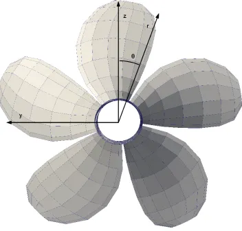
2.1 Propeller Cartesian and cylindrical coordinate systems (looking downstream) 3

3.1 Flow chart of numerical solution method . . . 8

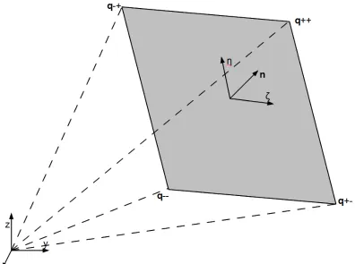
3.2 Hyperboloidal quadrilateral panel . . . 9

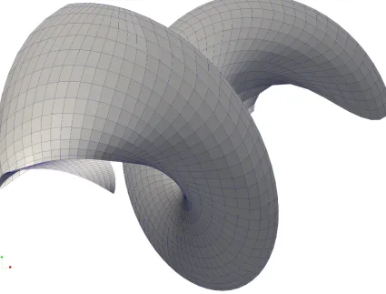
3.3 Panels on the blade, hub, and wake for the key blade . . . 10

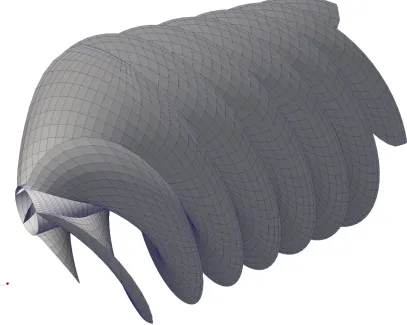
3.4 Panels on the blade, hub, and wake for the propeller . . . 11

3.5 Sketch of method used in numerical diﬀerentiation of the perturbation potential 17 3.6 Local panel coordinate systems . . . 17

4.1 Panels on Surface of a Sphere, 𝑁𝐶 =𝑁𝑆 = 9 . . . 22

4.2 Diﬀerence between the exact velocity potential and the numerical value . . . 23

4.3 𝑉𝛼 on surface of sphere, 𝑅𝑠𝑝ℎ𝑒𝑟𝑒 = 1, 𝑈∞ = 1 . . . 24

4.4 𝐶𝑃 on surface of sphere, 𝑅𝑠𝑝ℎ𝑒𝑟𝑒 = 1, 𝑈∞ = 1 . . . 25

4.5 Body and wake panels for medium numerical simulation, angle of attack zero 26 4.6 Velocity Magnitude on surface of foil for coarse, medium and ﬁne simulations 27 4.7 Velocity Magnitude on surface of foil for a range of span/chord ratios . . . . 28

4.8 Velocity Magnitude on surface of foil for 20, 40, and 80 wake panels . . . 29

5.1 Panels for coarse simulation,𝑁𝑆 =𝑁𝐶 = 5 . . . 32

5.2 Panels for medium simulation, 𝑁𝑆 =𝑁𝐶 = 7 . . . 32

5.3 Panels for ﬁne simulation, 𝑁𝑆 =𝑁𝐶 = 10 . . . 33

5.4 Panels for xﬁne simulation, 𝑁𝑆 =𝑁𝐶 = 14 . . . 33

5.5 𝐾𝑇 curves for B5-105, 𝑃/𝐷 = 0.8 . . . 34

5.6 𝐾𝑄 curves for B5-105, 𝑃/𝐷 = 0.8 . . . 35

A.1 Velocity Magnitude for B5-105, Coarse, 𝑃/𝐷= 0.8,𝐽 = 0.3 suction side (left) and pressure side (right) . . . 39

A.2 𝐶𝑃 for B5-105, Coarse, 𝑃/𝐷 = 0.8, 𝐽 = 0.3 suction side (left) and pressure side (right) . . . 39

A.3 Velocity Magnitude for B5-105, Coarse, 𝑃/𝐷= 0.8,𝐽 = 0.4 suction side (left) and pressure side (right) . . . 40

A.4 𝐶𝑃 for B5-105, Coarse, 𝑃/𝐷 = 0.8, 𝐽 = 0.4 suction side (left) and pressure side (right) . . . 40

(7)

A.6 𝐶𝑃 for B5-105, Coarse, 𝑃/𝐷 = 0.8, 𝐽 = 0.5 suction side (left) and pressure

side (right) . . . 41 A.7 Velocity Magnitude for B5-105, Coarse, 𝑃/𝐷= 0.8,𝐽 = 0.6 suction side (left)

and pressure side (right) . . . 42 A.8 𝐶𝑃 for B5-105, Coarse, 𝑃/𝐷 = 0.8, 𝐽 = 0.6 suction side (left) and pressure

side (right) . . . 42 A.9 Velocity Magnitude for B5-105, Medium, 𝑃/𝐷 = 0.8, 𝐽 = 0.3 suction side

(left) and pressure side (right) . . . 43 A.10𝐶𝑃 for B5-105, Medium, 𝑃/𝐷 = 0.8, 𝐽 = 0.3 suction side (left) and pressure

side (right) . . . 46 A.17 Velocity Magnitude for B5-105, Fine, 𝑃/𝐷 = 0.8, 𝐽 = 0.3 suction side (left)

and pressure side (right) . . . 47 A.18𝐶𝑃 for B5-105, Fine, 𝑃/𝐷 = 0.8,𝐽 = 0.3 suction side (left) and pressure side

(right) . . . 47 A.19 Velocity Magnitude for B5-105, Fine, 𝑃/𝐷 = 0.8, 𝐽 = 0.4 suction side (left)

(right) . . . 50 A.25 Velocity Magnitude for B5-105, xFine, 𝑃/𝐷= 0.8,𝐽 = 0.3 suction side (left)

and pressure side (right) . . . 51 A.26𝐶𝑃 for B5-105, xFine, 𝑃/𝐷 = 0.8, 𝐽 = 0.3 suction side (left) and pressure

(8)

A.27 Velocity Magnitude for B5-105, xFine, 𝑃/𝐷= 0.8,𝐽 = 0.4 suction side (left) and pressure side (right) . . . 52 A.28𝐶𝑃 for B5-105, xFine, 𝑃/𝐷 = 0.8, 𝐽 = 0.4 suction side (left) and pressure

side (right) . . . 52 A.29 Velocity Magnitude for B5-105, xFine, 𝑃/𝐷= 0.8,𝐽 = 0.5 suction side (left)

side (right) . . . 53 A.31 Velocity Magnitude for B5-105, xFine, 𝑃/𝐷= 0.8,𝐽 = 0.6 suction side (left)

(9)

List of Tables

(10)

List of Symbols

Δ𝜙 Potential diﬀerence across wake surface Ω Rotational speed of the propeller Φ Velocity potential

𝛼 Angle from free stream direction

𝜒(𝑟′) Blade rake as a function of𝑟′ 𝜖(𝜖𝑚𝑎𝑥, 𝑒𝑚𝑎𝑥, 𝑒) Camber of the blade

𝜖𝑚𝑎𝑥(𝑟′) Maximum camber of the a radial blade section, function of𝑟′

𝜂 Parametric variable in panel shape function

𝛾(𝑟′) Blade pitch angle as a function of𝑟′ 𝜙 Perturbation velocity potential

𝜙𝑗 Perturbation velocity potential at panel𝑗

𝜙+ Potential on the suction side of the wake 𝜙− Potential on the pressure side of the wake

𝜙±𝑗 Perturbation potential at the center of the suction(+) or

pressure(-) side trailing edge panels of the jth spanwise strip

𝜏(𝜏𝑚𝑎𝑥, 𝑒) Half thickness of the blade

𝜏𝑚𝑎𝑥 Maximum thickness of a radial blade section, function of 𝑟′

𝜃 Angle in𝑃 −𝑥𝑟𝜃

𝜃𝑘(𝑘) Angular location of the blade midchord at the hub of blade𝑘

𝜉(𝑟′) Blade skew as a function of𝑟′

(11)

Δ𝜙 Vector of perturbation potential diﬀerences around the trailing edge

ΔV Vector of velocity magnitude diﬀerences around the trailing edge

BP(𝑟′, 𝑒, 𝑘) Location of blade pressure face surface

BS(𝑟′, 𝑒, 𝑘) Location of blade suction face surface

c Unit vector in the𝑃 𝑛−𝑐𝑠 coordinate system described in the

𝑃 −𝑥𝑦𝑧 coordinate system

MC(𝑟′, 𝑘) Location of blade mid-chord line

nQ Surface normal vector at pointQ NT(𝑟′, 𝑘, 𝑒) Location of blade nose-tail line

n Surface normal vector

o Unit vector of the 𝑃 𝑛 −𝑜𝑝 Cartesian coordinate system de-scribed in the 𝑃 −𝑥𝑦𝑧 coordinate system

P(x,y,z) Arbitrary ﬁeld point

p Unit vector of the 𝑃 𝑛 −𝑜𝑝 Cartesian coordinate system de-scribed in the 𝑃 −𝑥𝑦𝑧 coordinate system

Q Vector locating a point on the surface𝑆

q0,q1, q2, & q3 Coeﬃcients of panel shape function

q++, q+−, q−+, & q−− Panel corner locations

Rijk Vector pointing from inﬂuenced panel 𝑖 to inﬂuencing panel 𝑗

on blade 𝑘

R =Q−P

s Unit vector in the𝑃 𝑛−𝑐𝑠 coordinate system described in the

Vinf Free stream velocity

VI Incident velocity on the propeller blade surface

𝑎 Coeﬃcient of 𝜙𝑐(𝑔) or 𝜙𝑠(𝑔)

(12)

𝐵𝑖𝑗 Inﬂuencing potential on panel 𝑖 from source distribution on

panel(s)𝑗

𝑐 Coeﬃcient of 𝜙𝑐(𝑔) or 𝜙𝑠(𝑔)

𝐶(𝑟′) Blade chord as a function of 𝑟′ 𝐶𝑃 Pressure coeﬃcient

𝐶𝑖𝑗 Inﬂuencing potential on panel 𝑖 from doublet distribution on

panel(s)𝑗

𝐸 Constant used in (2.8)

𝑒 Non-dimensional, unit chord, such that 0 is the leading edge and 1 is the trailing edge

𝑒𝑚𝑎𝑥(𝑟′) Location where the maximum camber occurs along the

nose-tail line, function of 𝑟′ 𝑓 Variable in (3.3)

𝑔 Distance along the blade surface

𝑔++ Distance from the center of the panel of interest to panel𝑚+ 2 𝑔± Linear distance between adjacent panel centers within a given

panel strip in the direction of increasing or decreasing panel index depending on the subscript

𝑖 Panel index

𝑗 Panel index

𝐾 Number of blades

𝑘 Blade number 1, 2,. . .𝐾

𝐿 Number of streamwise wake panels

𝑙 Index of streamwise wake panels

𝑚 panel index

𝑁 Number of panels on each propeller blade and the associated portion of the hub

𝑁𝐶 Number of blade panels in the chordwise direction (streamwise

(13)

𝑁𝑆 Number of blade panels in the spanwise direction

(circumfer-ential for sphere)

𝑃 −𝑥𝑟𝜃 Propeller cylindrical coordinate system

𝑃 −𝑥𝑦𝑧 Propeller cartesian coordinate system

𝑃𝐼 Pressure at the propeller center

𝑃 𝑛−𝑐𝑠 Panel coordinate system

𝑃 𝑛−𝑜𝑝 Panel Cartesian coordinate system

𝑄𝑊 Point on wake surface

𝑅 Propeller radius

𝑟 Radial distance from center of sphere

𝑟 Radial distance from x-axis in 𝑃 −𝑥𝑟𝜃 𝑟′ non-dimensional propeller radius

𝑅𝐻 Propeller hub radius

𝑅𝑠𝑝ℎ𝑒𝑟𝑒 Sphere radius

𝑆 Combined blade, hub, and wake surfaces

𝑠1 Panel geometry parameter used in Equations (3.14) & (3.15) 𝑠2 Panel geometry parameter used in Equations (3.14) & (3.15) 𝑠3 Panel geometry parameter used in Equations (3.14) & (3.15) 𝑆𝐵 Propeller blade surface

𝑆𝐻 Propeller hub surface

𝑆𝑗 Surface area of panel 𝑗

𝑆𝑊 Propeller wake surface

𝑆𝐿𝐴𝐸1 First system of linear algebraic equations

𝑆𝐿𝐴𝐸2 Second system of linear algebraic equations 𝑢 Spanwise panel index (circumferential for sphere)

(14)

𝑣 Chordwise panel index (streamwise for sphere)

𝑣𝑐 Perturbation velocity in the panel chordwise direction

𝑣𝑜 Perturbation velocity in the panel𝑜 direction

𝑣𝑝 Perturbation velocity in the panel𝑝 direction

𝑣𝑠 Perturbation velocity in the panel spanwise direction

𝑉±𝑗 Velocity magnitude at the center of the suction(+) or

pressure(-) side trailing edge panels of the jth spanwise strip

𝑊_𝑖𝑗𝑇 𝐸 Inﬂuencing potential on panel 𝑖 from doublet distribution on

wake panel(s) 𝑗

𝑥 Distance along the x-axis in𝑃 −𝑥𝑦𝑧 and 𝑃 −𝑥𝑟𝜃 𝑦 Distance along the y-axis in𝑃 −𝑥𝑦𝑧

(15)

Abstract

This report describes the governing equation and boundary conditions for a marine propeller operating in a uniform flow field of inviscid and irrotational fluid. A method is presented by which the velocity and pressure on the blade surface of the propeller can be numerically simulated, using hyperboloidal, constant strength source and doublet panels. Accuracy of the numerical method is verified through comparison with analytically known results and the ability of the numerical simulation to predict the thrust and torque on a propeller in open water is assessed through comparison with published experimental results. The thrust and torque results for the propeller are near the experimental measurements but do not converge to a common value as the panel size decreases.

(16)

1 Introduction

(17)

2 The Propeller Flow Problem

2.1 Propeller Geometry and Coordinate System

We deﬁne the propeller Cartesian coordinate system𝑃−𝑥𝑦𝑧such that the𝑥-axis is concentric with the shaft axis and positive downstream, the 𝑧-axis extends upward from the shaft centerline bisecting the nose-tail line of a blade section at the propeller hub, and the 𝑦-axis is such that we have a right handed coordinate system. It will be convenient to deﬁne a cylindrical propeller coordinate system 𝑃 −𝑥𝑟𝜃 such that the 𝑥-axis is the same as that of

𝑃 −𝑥𝑦𝑧 but where𝑟 is the radial distance from the𝑥-axis and 𝜃 increases moving clockwise from the𝑧-axis, looking downstream. The cylindrical coordinate system can be transformed into the Cartesian system 𝑃 −𝑥𝑦𝑧 using the following relations:

𝑥=𝑥 (2.1)

𝑦 =−𝑟sin𝜃 (2.2)

𝑧 =𝑟cos𝜃 (2.3)

The midchord line at any radius can be located using the following relations:

MC(𝑟′, 𝑘) =

⎡ ⎣ 𝑀 𝐶𝑥 𝑀 𝐶𝑦 𝑀 𝐶𝑧 ⎤ ⎦= ⎡ ⎣ 𝜒(𝑟′)

−𝑟sin(

𝜉(𝑟′) +𝜃𝑘(𝑘)

)

𝑟cos(𝜉(𝑟′) +𝜃𝑘(𝑘)

) ⎤ ⎦ (2.4) where: 𝑟′ = 𝑟−𝑅𝐻 𝑅−𝑅𝐻

𝑅 is the propeller radius

𝑅𝐻 is the propeller hub radius

𝜃𝑘(𝑘) is the angular location of the blade midchord at the hub of blade 𝑘, with respect

to the z-axis

𝑘 is the blade number 1, 2,. . . ,𝐾 𝐾 is the number of blades

(18)

(19)

The nose-tail line can be located using the following relationship:

NT(𝑟′, 𝑘, 𝑒) =

⎡ ⎣ 𝑁 𝑇𝑥 𝑁 𝑇𝑦 𝑁 𝑇𝑧 ⎤ ⎦= ⎡ ⎢ ⎢ ⎢ ⎣ 𝜒(𝑟′) + (

𝑒𝐶(𝑟′)−𝐶(₂𝑟′))sin𝛾(𝑟′)

−𝑟sin(𝜉(𝑟′) +𝜃𝑘(𝑘) +

(_𝑒𝐶₍_𝑟′₎

𝑟 −

𝐶(𝑟′₎

2𝑟

)

cos𝛾(𝑟′))

𝑟cos(𝜉(𝑟′) +𝜃𝑘(𝑘) +

( 𝑒𝐶(𝑟′) 𝑟 − 𝐶(𝑟′) 2𝑟 )

cos𝛾(𝑟′))

⎤ ⎥ ⎥ ⎥ ⎦ (2.5) where:

𝐶(𝑟′) is the blade chord length as a function of 𝑟′

𝑒 is the non-dimensional, unit chord, such that 0 is the leading edge and 1 is the trailing edge

𝛾(𝑟′) is the blade pitch angle as a function of𝑟′

It should be noted that for a propeller the chord 𝐶(𝑟′) is the length between a leading edge point and a trailing edge point along a plane of constant radius, thus 𝐶 is the length of an arc measured along a helix. Also, here the blade pitch angle 𝛾 is the geometric pitch angle measured along the nose-tail line of the blade section.

The blade section shape at any radius can be described by a half-thickness shape function

𝜏(𝜏𝑚𝑎𝑥, 𝑒) and a camber shape function 𝜖(𝜖𝑚𝑎𝑥, 𝑒𝑚𝑎𝑥, 𝑒), where:

𝜏𝑚𝑎𝑥 is the maximum thickness of the section and is a function of 𝑟′

𝜖𝑚𝑎𝑥 is the maximum camber of the section and is a function of𝑟′

𝑒𝑚𝑎𝑥 is the location where the maximum camber thickness occurs along the nose-tail

line and is also a function of𝑟′

These section shape functions are analogous to those used to describe foil section series, like the NACA series. Using them we can locate the blade surface with the following equations:

BS(𝑟′, 𝑒, 𝑘) =

⎡

⎢ ⎣

𝑁 𝑇𝑥(𝑟′, 𝑒, 𝑘)−𝜏sin𝛼sin𝛾−𝜖cos𝛾−𝜏cos𝛼cos𝛾

−𝑟sin(𝜉+𝜃𝑘+

(_𝑒𝐶

𝑟 − 𝐶

2𝑟

)

cos𝛾−𝜏sin𝛼

𝑟 cos𝛾+ 𝜖

𝑟sin𝛾+ 𝜏cos𝛼

𝑟 sin𝛾

)

𝑟cos(𝜉+𝜃𝑘+

(_𝑒𝐶

𝑟 − 𝐶

2𝑟

)

cos𝛾−𝜏sin𝛼

𝑟 cos𝛾+ 𝜖

𝑟sin𝛾+ 𝜏cos𝛼

𝑟 sin𝛾

) ⎤

⎥ ⎦

(2.6)

BP(𝑟′, 𝑒, 𝑘) =

⎡

⎢ ⎣

𝑁 𝑇𝑥(𝑟′, 𝑒, 𝑘)−𝜏sin𝛼sin𝛾−𝜖cos𝛾+𝜏cos𝛼cos𝛾

−𝑟sin(𝜉+𝜃𝑘+

(_𝑒𝐶

𝑟 − 𝐶

2𝑟

)

cos𝛾+𝜏sin_𝑟 𝛼cos𝛾+_𝑟𝜖sin𝛾−𝜏cos𝛼 𝑟 sin𝛾

)

𝑟cos(𝜉+𝜃𝑘+

(_𝑒𝐶

𝑟 − 𝐶

2𝑟

)

cos𝛾+𝜏sin_𝑟 𝛼cos𝛾+_𝑟𝜖sin𝛾−𝜏cos𝛼 𝑟 sin𝛾

) ⎤

⎥ ⎦

(20)

2.2 Velocity Potential and Boundary Conditions

The ﬂow ﬁeld in which the propeller operates can be described by the linear combination of a free-stream velocity potential and a perturbation velocity potential 𝜙 which both satisfy the Laplace Equation.

∇2𝜙 = 0

The perturbation potential also must become zero at an inﬁnite distance away from the propeller.

Consider a boundary surface 𝑆 which consists of a propeller blade surface 𝑆𝐵, a hub

surface 𝑆𝐻 and a wake surface 𝑆𝑊 with normal vector n pointing into the ﬂuid domain.

Applying Green’s identity, the perturbation velocity potential𝜙 at any ﬁeld point P(𝑥, 𝑦, 𝑧) can be found from a distribution of sources and doublets on the surface 𝑆. The relationship for 𝜙 can be written as follows [2]:

4𝜋𝐸𝜙(P) =

∫ ∫

𝑆

𝜙(Q) ∂

∂nQ

(

1

𝑅(P,Q)

) 𝑑𝑆−

∫ ∫

𝑆

∂𝜙(Q)

∂nQ

⋅ 1

R(P,Q)𝑑𝑆 (2.8) where

𝐸 =

⎧ ⎨

⎩

0 for the point Pinside S,(not in the ﬂuid domain) 1/2 for the point Pon S,

1 for the point Poutside S,(in the ﬂuid domain)

Q is a vector locating a point on the surface 𝑆

nQ is the normal vector at pointQ pointing into the ﬂuid domain R =Q−P

∂

∂nQ is the normal derivative at Q

The solution of equation (2.8) is made unique through the application of a kinematic boundary condition, imposed on 𝑆𝐵 and𝑆𝐻 such that the normal velocity on those surfaces

is zero. This can be expressed through equation (2.9).

∂𝜙(Q)

∂nQ

=−VI ⋅nQ =−(Vinf +Ω×Q)⋅nQ (2.9)

where Vinf is the free stream velocity, Ω is the rotational speed of the propeller, and VI

is the resultant incident velocity on the propeller blade surface. Imposing the kinematic boundary condition in (2.9), the second term on the right hand side of equation (2.8) can be satisﬁed using a constant source distribution on surfaces 𝑆𝐵 and 𝑆𝐻.

We assume that there is no ﬂow through nor a pressure jump across the wake surface

𝑆𝑊, however a discontinuity of the potential Δ𝜙 is allowed. For the steady problem, Δ𝜙 is

constant along any stream line in the wake and can be written as

(21)

where𝜙+is the potential on the suction side of the wake and𝜙−the potential on the pressure

side.

Applying the kinematic boundary condition via equation (2.9) and the wake boundary condition via equation (2.10) to equation (2.8) we get equation (2.11) as per Hoshino [2].

2𝜋𝐸𝜙(P)− ∫ ∫

𝑆𝐵+𝑆𝐻

𝜙(Q) ∂

∂nQ

(

1

R(P,Q)

) 𝑑𝑆

− ∫ ∫

𝑆𝑊

Δ𝜙(QW)

∂ ∂nQW

(

1

R(P,Q)

) 𝑑𝑆

=

∫ ∫

𝑆𝐵+𝑆𝐻

(VI⋅nQ)

1

R(P,Q)𝑑𝑆 (2.11) Here 𝑄𝑊 indicates a point on the wake surface. Integrals over 𝑆𝐵 and 𝑆𝐻 are Cauchy

(22)

3 Discretization and Numerical

Method

Figure 3.1 illustrates the process used to numerically solve the propeller ﬂow problem sat-isfying the Kutta condition. The important steps of this process will be detailed in this chapter.

3.1 Discretization of the Blade, Hub, and Wake

Sur-faces

The blade, hub, and wake surfaces will be discretized into a number of quadrilateral panels. The panel shape and any point on the panel surface is described by Morino [10] via equations (3.1) and (3.2), creating a hyberboloidal quadrilateral panel.

Q=q0+𝜁q1+𝜂q2+𝜁𝜂q3 (3.1) ⎡ ⎢ ⎢ ⎣ q0 q1 q2 q3 ⎤ ⎥ ⎥ ⎦ = 1 4 ⎡ ⎢ ⎢ ⎣

1 1 1 1 1 1 −1 −1 1 −1 1 −1 1 −1 −1 1

⎤ ⎥ ⎥ ⎦ ⎡ ⎢ ⎢ ⎣ q++

q+−

q−+

q−− ⎤ ⎥ ⎥ ⎦ (3.2)

Hereq++,q+−,q−+, andq−−are corner points of a panel and𝜁 and𝜂 are local parametric

variables with the domain𝜁, 𝜂 ∈[−1,1]. Figure 3.2 illustrates a typical panel and ﬁgure 3.3 shows an example of a discretized blade, the hub surface between it and an adjacent blade, and the associated wake surface. It is important to note that these panels are not planar and that their bounding edges may be twisted, allowing all panel corners to lay on the blade surface, increasing the accuracy in which the blade is modeled.

Using equations (2.6) and (2.7) to ﬁnd the panel corners we can discretize the propeller hub and blades through systematic variations of𝑟′ and 𝑒. The blade will be divided into𝑁𝑆

panels spanwise and 𝑁𝐶 panels chordwise on each side of the blade, giving 2𝑁𝑆𝑁𝐶 panels

per blade. We will use a cosine spacing in the spanwise direction and a uniform spacing in the chordwise direction such that

𝑟′ = 1/2− 1

(23)

(24)

(25)

(26)

(27)

where 𝑓 = ⎧  ⎨  ⎩

0 for𝑢= 1 (2𝑢−1)𝜋

2(𝑁𝑆+ 1)

for𝑢= 2, 3,. . . , 𝑁𝑆 + 1

and

𝑒= 𝑣

𝑁𝐶

(3.4) where 𝑣 = 0, 1, . . . , 𝑁𝐶.

The hub surface has been discretized in the chordwise direction using the same uniform spacing that is used discretize the root section of the blade. The corner points of the hub panels lay on helical arcs which connect the corners of the blade root panels on the suction side of one blade to the corners of blade root panels on the pressure side of the adjacent blade. These helical arcs are uniformly divided into 𝑁𝑆 panels, creating 𝑁𝑆𝑁𝐶 panels on

the hub section between each blade. An example of the hub panels can be seen in ﬁgure 3.3. The blade wake has been approximated by strips of constant strength doublet panels emanating from the pairs of trailing edge panels on the blade surface. These panels continue downstream from the trailing edge with a constant pitch equal to the geometric pitch𝛾 of the blade at that radius. Each wake panel represents a 4

3𝑁𝑆 radian angular displacement around

the helix of that wake strip, thus the panel size on a given radial wake strip is constant along the helix of the that wake strip. Each wake strip consists of 𝐿 panels.

3.2 First System of Linear Algebraic Equations

Having divided the blade and hub surfaces 𝑆𝐵 and 𝑆𝐻 into 𝐾 ×𝑁 panels we can write

equation (2.11) as a system of 𝑁 linear algebraic equations. Here N is the number of panels on the key blade and its surrounding hub section. Due to the symmetry of the steady propeller problem we need only solve for the perturbation potential on one blade and its surrounding hub section, accounting for the inﬂuence of the other propeller surfaces on that key blade. 𝜙𝑗 and VI⋅nQ are assumed to be constant within each panel and equal to the

value at the centroid of the panel. The ﬁrst system of linear equations 𝑆𝐿𝐴𝐸1 then can be

written as 𝑁 ∑ 𝑗=1 (𝛿𝑖𝑗 −𝐶𝑖𝑗)𝜙𝑗 = 𝑁 ∑ 𝑗=1

𝐵𝑖𝑗(VI⋅nQ) (3.5)

for 𝑖= 1, 2, . . . , 𝑁

The source and body doublet inﬂuence coeﬃcients are written as 𝐵𝑖𝑗 and 𝐶𝑖𝑗 respectively.

In equation (3.5), the 𝑖 index refers to the row of the system matrix and the point being affected by the influence coefficient. The 𝑗 index indicates the influencing panel and the column in the left hand side matrix. The source and body doublet influence coefficients,𝐵𝑖𝑗

and 𝐶𝑖𝑗, include the inﬂuence from sister panels on all blades onto the collocation point on

(28)

blade is included. In equation (3.5) 𝛿 is the Kronecker delta.

𝑆𝐿𝐴𝐸1 is merely solved as the initial condition in the iterative method used to satisfy

the Kutta condition. The solution of 𝑆𝐿𝐴𝐸1 does not include the inﬂuence of the wake nor

does it satisfy the Kutta condition.

After solving 𝑆𝐿𝐴𝐸1 we will calculate and store two vectors Δ𝜙 and ΔV, both with

dimension 𝑁𝑆, to be used in the iterative satisfaction of the Kutta condition.

Δ𝜙= ⎡ ⎢ ⎢ ⎢ ⎣

Δ𝜙1

Δ𝜙2

.. . Δ𝜙𝑁𝑆 ⎤ ⎥ ⎥ ⎥ ⎦ = ⎡ ⎢ ⎢ ⎢ ⎣

𝜙+1𝑇 𝐸 −𝜙₋₁𝑇 𝐸

𝜙+2𝑇 𝐸 −𝜙₋₂𝑇 𝐸

.. . 𝜙₊_𝑁𝑇 𝐸 𝑆 −𝜙−𝑁𝑆𝑇 𝐸 ⎤ ⎥ ⎥ ⎥ ⎦ ΔV= ⎡ ⎢ ⎢ ⎢ ⎣ Δ𝑉1

Δ𝑉2

.. . Δ𝑉𝑁𝑆 ⎤ ⎥ ⎥ ⎥ ⎦ = ⎡ ⎢ ⎢ ⎢ ⎣

𝑉+1𝑇 𝐸 −𝑉₋₁𝑇 𝐸

𝑉₊₂𝑇 𝐸 −𝑉₋₂𝑇 𝐸

.. . 𝑉₊_𝑁𝑇 𝐸 𝑆 −𝑉−𝑁 𝑇 𝐸 𝑆 ⎤ ⎥ ⎥ ⎥ ⎦

Where𝜙±𝑗𝑇 𝐸 and𝑉_±_𝑗𝑇 𝐸 are the perturbation potential and velocity magnitude at the center

of the suction(+) or pressure(-) side trailing edge panels of the jth spanwise strip. The 𝑇 𝐸

subscript indicates that the value appears only when panel𝑗 is a trailing edge panel.

3.3 Second System of Linear Algebraic Equations

In our second system of linear algebraic equations 𝑆𝐿𝐴𝐸2, we have included the inﬂuence

of the wake 𝑊_𝑖𝑗𝑇 𝐸 on the right hand side of the system and will specify values of Δ𝜙_𝑗𝑇 𝐸

attempting to satisfy the Kutta condition. Here again the 𝑇 𝐸 subscript indicates that the wake inﬂuence is only added when panel 𝑗 is a trailing edge panel. The manner in which values of Δ𝜙_𝑗𝑇 𝐸 are chosen is discussed later in this chapter.

𝑁 ∑ 𝑗=1 (𝛿−𝐶𝑖𝑗)𝜙𝑗 = 𝑁 ∑ 𝑗=1 [

𝐵𝑖𝑗(VI⋅nQ) +𝑊𝑖𝑗𝑇 𝐸Δ𝜙_𝑗𝑇 𝐸 ]

(3.6)

for 𝑖= 1, 2, . . . , 𝑁

The wake influence coefficient 𝑊𝑖𝑗𝑇 𝐸 is the influence of an entire streamwise wake strip

(29)

3.4 Inﬂuence Coeﬃcients

The influence coefficients used in equations (3.5) and (3.6) and the manner in which effects from the other blades have been taken into account is show below. We see that the influence of multiple blades is conglomerated into a single coefficient. The influence of each wake panel in a streamwise strip is accounted for in the same manner.

𝐶𝑖𝑗 = 𝐾 ∑ 𝑘=1 [ 1 2𝜋 ∫ ∫ 𝑆𝑗 ∂ ∂nj

( 1 Rijk ) 𝑑𝑆𝑗 ] (3.7) 𝑊𝑖𝑗 = 𝐾 ∑ 𝑘=1 𝐿 ∑ 𝑙=1 [ 1 2𝜋 ∫ ∫ 𝑆𝑗 ∂ ∂nj

( 1 Rijk ) 𝑑𝑆𝑗 ] (3.8) 𝐵𝑖𝑗 = 𝐾 ∑ 𝑘=1 [ − 1 2𝜋 ∫ ∫ 𝑆𝑗 ( 1 Rijk ) 𝑑𝑆𝑗 ] (3.9)

Rijk is here deﬁned as

Rijk =Qjk(𝜁, 𝜂)−Pi (3.10)

We also deﬁne;

s1(𝜁, 𝜂) =

∂Q(𝜁, 𝜂)

∂𝜁 (3.11)

s2(𝜁, 𝜂) =

∂Q(𝜁, 𝜂)

∂𝜂 (3.12)

s3(𝜁, 𝜂) =

s1×s2

∣s1×s2∣

(3.13) Using the termsR,s1, s2, and s3 we deﬁne the following as per Hsin [4].

𝐼𝐷(𝜁, 𝜂) =

1 2𝜋tan

−1 (

(R×s1)⋅(R×s2)

∣R∣∣R⋅(s1×s2)∣

) (3.14) 𝐼𝑆(𝜁, 𝜂) =− 1 2𝜋 {

−(R×s1)⋅s3(0,0) ∣s1∣

sinh−1

(

R⋅s1

∣R×s1∣

)

+ (R×s2)⋅s3(0,0)

∣s2∣

sinh−1

(

R⋅s2

∣R×s2∣

)}

(3.15)

and

𝜖(𝜁, 𝜂) = R⋅(s1 ×s2

∣R⋅(s1 ×s2∣

(30)

such that, Φ𝐷 = 1 2𝜋 ∫ ∫ 𝑆𝑗 ∂ ∂nj

( 1 Rijk ) 𝑑𝑆𝑗 = ⎧ ⎨ ⎩

0 If,𝐼𝐷(1,1) +𝐼𝐷(1,−1) +𝐼𝐷(−1,1) +𝐼𝐷(−1,−1) = 1

𝜑𝐷 − 1₂_∣_𝜑𝜑_𝐷𝐷_∣ If,𝜖(1,1)𝜖(1,−1)𝜖(−1,1)𝜖(−1,−1)<0

𝜑𝐷 Else

(3.17)

where

𝜑𝐷 = 𝜖(1,1)𝐼𝐷(1,1) − 𝜖(1,−1)𝐼𝐷(1,−1) − 𝜖(−1,1)𝐼𝐷(−1,1) + 𝜖(−1,−1)𝐼𝐷(−1,−1)

(3.18) and − 1 2𝜋 ∫ ∫ 𝑆𝑗 ( 1 Rijk )

𝑑𝑆𝑗 =𝐼𝑆(1,1)−𝐼𝑆(1,−1)−𝐼𝑆(−1,1) +𝐼𝑆(−1,−1)

+ (R(0,0)⋅s3(0,0)) Φ𝐷 (3.19)

3.5 Satisfaction of the Kutta Condition

The iterative process through which the Kutta condition is satisfied is illustrated in figure 3.1 and we will refer to that illustration in this description of the process. The Kutta condition must be satisfied at every spanwise set of trailing edge panels and to accomplish this we will choose a vector Δ𝜙 such that every term of vector ΔV is zero.

As illustrated in ﬁgure 3.1, once 𝑆𝐿𝐴𝐸1 is solved, the initial vectors Δ𝜙 and ΔV are

obtained from the solution. We will identify this set of potential and velocity vectors by the superscript 0. Arbitrarily modifying Δ𝜙0, we create a new vector Δ𝜙1, the terms of which will be used to compute the wake inﬂuence in 𝑆𝐿𝐴𝐸2. Solving𝑆𝐿𝐴𝐸2 with the wake

inﬂuence scaled by Δ𝜙1, we obtain another set of velocity diﬀerentials at the trailing edge

ΔV1.

If every component of ΔV1 does not vanish, we must estimate a new potential diﬀerence for each pair of trailing edge panels, Δ𝜙_{𝑛𝑒𝑤𝑗}𝑇 𝐸, which will make Δ𝑉_𝑗𝑇 𝐸 = 0 for that pair.

Using our two sets of vectors Δ𝜙0, ΔV0, Δ𝜙1, and ΔV1, we can linearly model the rela-tionship between Δ𝜙𝑗𝑇 𝐸 and Δ𝑉_𝑗𝑇 𝐸 at each spanwise set of trailing edge panels and solve for

the potential diﬀerence Δ𝜙_𝑗𝑇 𝐸 which will make Δ𝑉_𝑗𝑇 𝐸 = 0. Δ𝜙_𝑗𝑇 𝐸 is calculated and 𝑆𝐿𝐴𝐸₂

is solved for each spanwise set of trailing edge panels individually. After 𝑆𝐿𝐴𝐸2 has been

solved for every spanwise pair of trailing edge panels, the vector ΔV is checked to see if every component is suﬃciently close to zero.

(31)

3.6 Calculation of Velocity and Pressure on the Blade

Surface

The velocities on the blade surfaces are obtained through numerical diﬀerentiation. This diﬀerentiation is done with respect to the local panel coordinate system, the perturbation velocity is combined with the free stream velocity, and the resultant converted to the propeller Cartesian coordinate system.

The perturbation potential ﬁeld on the blade surface is modeled as two quadratic poly-nomials, 𝜙𝑐(𝑔) and 𝜙𝑠(𝑔), in the chordwise and spanwise directions respectively. Here 𝑔 is

the distance along the blade surface in either the chordwise or spanwise direction. The co-eﬃcients of the quadratic function are obtained from the solution of equation (3.20) for 𝑎,

𝑏, and 𝑐.

⎡

⎣

0 0 1

𝑔2₊ 𝑔+ 1 𝑔2

− 𝑔− 1

⎤ ⎦ ⎡ ⎣ 𝑎 𝑏 𝑐 ⎤ ⎦= ⎡ ⎣ 𝜙𝑚

𝜙𝑚+1 𝜙𝑚−1

⎤

⎦ (3.20)

Here𝑚is either the spanwise panel index 𝑢or the chordwise panel index𝑣 depending on the direction for which the quadratic function is being ﬁt. 𝜙𝑚 is the perturbation potential

at the center of the panel where the velocity is being computed, and 𝜙𝑚±1 indicates an

adjacent panel with either an increasing or decreasing panel index. In equation (3.20) 𝑔± is

the linear distance between adjacent panel centers within a given panel strip in the direction of increasing or decreasing panel index depending on the subscript. Figure 3.5 illustrates this curve ﬁtting for a simple case.

For the calculation of the velocity on a panel at the edge of the blade, where there is only one adjacent panel per strip, the diﬀerentiation is shifted. In an example where there is no panel index less than 𝑚, the system of equations describing the potential polynomial is similar to equation (3.20), however the panel of decreasing index has been replaced by a panel of index two greater than the panel of interest; as seen in equation (3.20). This eﬀectively shifts the domain of the quadratic equation in the direction of increasing panel index.

⎡

⎣

0 0 1

𝑔2₊ 𝑔+ 1 𝑔2

++ 𝑔++ 1 ⎤ ⎦ ⎡ ⎣ 𝑎 𝑏 𝑐 ⎤ ⎦= ⎡ ⎣ 𝜙𝑚

𝜙𝑚+1 𝜙𝑚+2

⎤

⎦ (3.21)

Here 𝑔++ is the distance from the center of the panel of interest to panel 𝑚+ 2, and 𝜙𝑚+2

is the perturbation potential at panel 𝑚+ 2. The same shift can be done in the opposite direction for the case where there is no panel with index greater than the panel where the velocity is to be computed.

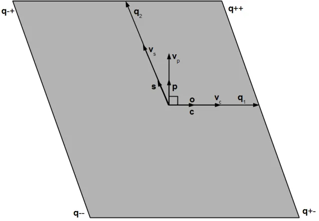
The derivatives of𝜙𝑐(𝑔) and𝜙𝑠(𝑔) with respect to𝑔 are the perturbation velocities in the

chordwise and spanwise directions, 𝑣𝑐 and 𝑣𝑠. 𝑣𝑐 and 𝑣𝑠 are assumed to act in the direction

of q1 and q2 respectively. We create a panel coordinate system 𝑃 𝑛−𝑐𝑠 with unit vectors c and s in the direction of q1 and q2 respectively. c and s are not always normal to each

(32)

Figure 3.5: Sketch of method used in numerical diﬀerentiation of the perturbation potential

(33)

system 𝑃 𝑛−𝑜𝑝 to be combined with the incident velocityVI. Coordinate systems𝑃 𝑛−𝑐𝑠

and 𝑃 𝑛−𝑜𝑝 are illustrated in ﬁgure 3.6. Figure 3.6 shows that o=c. The projection onto the 𝑃 𝑛−𝑜𝑝 coordinate system is accomplished through equations (3.22) and (3.23).

𝑣𝑜 =𝑣𝑐 (3.22)

𝑣𝑝 =

𝑣𝑠−(s⋅o)𝑣𝑐

s⋅p (3.23)

where:

s is a unit vector in the direction ofq2

o is a unit vector of the 𝑃 𝑛 −𝑜𝑝 Cartesian coordinate system described in the

p is a unit vector of the 𝑃 𝑛 −𝑜𝑝 Cartesian coordinate system described in the

Thus, the total velocity at the the panel center, in the panel Cartesian coordinate system is given by equation (3.24). The component normal to the panel surface is zero due to the application of the kinematic boundary condition on the blade surface.

V =

⎡

⎣

VI⋅o+𝑣𝑜 VI⋅p+𝑣𝑝

0

⎤

⎦ (3.24)

The pressure on a panel is obtained using the Bernoulli equation such that

𝑃 =𝑃𝐼+

1 2𝜌(∣VI∣

2_{− ∣}_V_∣2₎ _(3.25)

where 𝑃𝐼 is the reference pressure at the propeller center.

The pressure coeﬃcient 𝐶𝑃 follows as:

𝐶𝑃 = 1−

∣V∣ ∣VI∣

(3.26)

3.7 Calculation of Propeller Forces

The thrust 𝐹𝑥 and the torque 𝑀𝑥 acting on the propeller are obtained by integrating the

pressure and viscous forces on the blade surfaces.

𝐹𝑥=𝐾 𝑁

∑

𝑗=1

(34)

𝑀𝑥 =𝐾 𝑁

∑

𝑗=1

[(𝑃𝑗Δ𝐴𝑧𝑦−𝑃𝑗Δ𝐴𝑦𝑧) + (𝐹𝜈𝑧𝑦−𝐹𝜈𝑦𝑧)] (3.28)

Where

𝑃𝑗 is the pressure at panel j

ΔA =−nΔ𝐴, subscript indicates component direction Δ𝐴 is the panel area

F𝜈 is the viscous force vector, subscript indicates component direction

𝑦, 𝑧 panel center location in propeller Cartesian coordinate system𝑃 −𝑥𝑦𝑧

The magnitude of the viscous force per panel is equal to 1

2𝜌𝐶𝐹Δ𝐴𝑉

2 _(3.29)

where 𝐶𝐹 is the ITTC friction coeﬃcient [9] and 𝑉 is the velocity magnitude on the panel.

The viscous forces are assumed to act in the direction of the local velocity vector.

The advance ratio, thrust coefficient, torque coefficient and open-water efficiency are defined as

𝐽 = 𝑉𝐼𝑥

𝑛𝐷 (3.30)

𝐾𝑇 =

𝐹𝑥

𝜌𝑛2_𝐷4 (3.31) 𝐾𝑄 =

𝑀𝑥

(35)

4 Veriﬁcation of the Method and

Code

4.1 Sphere in Uniform Flow

Katz and Plotkin [5] describe the velocity potential field around a sphere in an otherwise uniform flow field as,

Φ =𝑈∞cos𝛼

( 𝑟+𝑅

3

𝑠𝑝ℎ𝑒𝑟𝑒

2𝑟2 )

(4.1) the resulting velocity ﬁeld as,

V𝑟 =𝑈∞cos𝛼

(

1−𝑅 3

𝑟3 )

(4.2)

V𝛼 =−𝑈∞sin𝛼

(

1 + 𝑅

3

2𝑟3 )

(4.3) and the coeﬃcient of pressure 𝐶𝑃 on the sphere surface as

𝐶𝑃 =

(

1− 9

4sin

2 𝛼

)

(4.4)

𝑈∞ is the free stream velocity, 𝑅𝑠𝑝ℎ𝑒𝑟𝑒 is the radius of the sphere, 𝑟 is the radial distance

from the center of the sphere and 𝛼 is the angle from the free-stream ﬂow. In each of the equations above, the ﬁrst term inside the parenthesis is the contribution from the free-stream and the second term represents the perturbation caused by the sphere.

To verify the accuracy of the method described in Chapter 3, a grid convergence study was performed using a sphere as the geometry, so that the results could be compared with equations (4.1) - (4.3). A sphere of unit radius was discretized using equations (4.5) - (4.7) to determine location of the panel corners in a Cartesian coordinate system with the origin at the center of the sphere.

𝑥=−𝑅𝑠𝑝ℎ𝑒𝑟𝑒cos

( 𝑣𝜋 𝑁𝐶

)

(36)

𝑦=

{

−0.001 cos(_𝑁𝑢𝜋

𝑆) If 𝑣 = 0 or 𝑁𝐶,

−𝑅𝑠𝑝ℎ𝑒𝑟𝑒sin(_𝑁𝑣𝜋 𝐶) cos(

𝑢𝜋

𝑁𝑆) Else.

(4.6)

𝑧 =

{

−0.001 sin(_𝑁𝑢𝜋

𝑆) If 𝑣 = 0 or 𝑁𝐶,

−𝑅𝑠𝑝ℎ𝑒𝑟𝑒sin(_𝑁𝑣𝜋 𝐶) sin(

𝑢𝜋

𝑁𝑆) Else.

(4.7)

Where

𝑅𝑠𝑝ℎ𝑒𝑟𝑒 = Radius of the sphere

𝑁𝐶 = number of streamwise panels on half of the sphere

𝑁𝑆 = number of circumferential panels on half of the sphere

𝑢 = 0, 1,. . . ,𝑁𝑆

𝑣 = 0, 1,. . . ,𝑁𝐶

The special case where 𝑣 equals either zero or 𝑁𝐶 has been implemented to insure that no

panel corners are co-located, which causes one of the principal vectors used to compute the panel inﬂuence functions to become degenerate.

The other half of the sphere is paneled by mirroring the panel corners about the X-Y plane. The term _𝑁𝑣𝜋

𝐶 in equations (4.5) - (4.7) is equal to 𝛼 in equations (4.1) - (4.3) thus

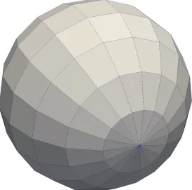
panel centers are located at intervals of 𝜋/𝑁𝐶 streamwise around the sphere. Figure 4.1

illustrates the panel arrangement on a sphere where 𝑁𝐶 = 𝑁𝑆 = 9. No wake has been

modeled for this problem as no lift is developed.

Figure 4.2 shows the diﬀerence between the perturbation potential from equation (4.1) and the numerical results at panels centers, plotted over half of the sphere. Results are given for cases where𝑁𝐶 =𝑁𝑆 = 3,9,& 27. From ﬁgure 4.2 one can see that the results converge

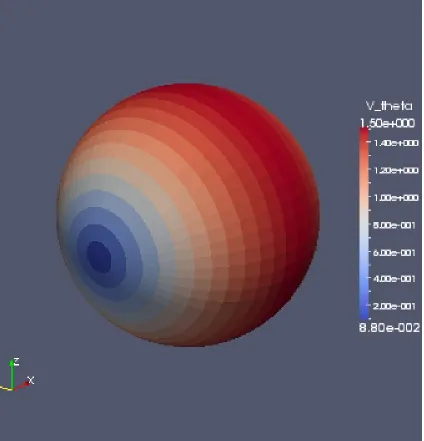
rapidly to equation (4.1) as the number of panels is increased. Figures 4.3 and 4.4 show values of 𝑉𝜃 and 𝐶𝑃 on a sphere of unit radius in a unit free stream ﬂow. The maximum

and minimum values that occur for the quantities shown are printed at the top and bottom of the color scale. The sphere in ﬁgures 4.3 and 4.4 has been paneled with parameters 𝑁𝐶

(37)

(38)

(39)

(40)

(41)

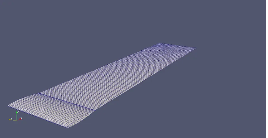
Figure 4.5: Body and wake panels for medium numerical simulation, angle of attack zero

4.2 Van de Vooren Airfoil in Uniform Flow

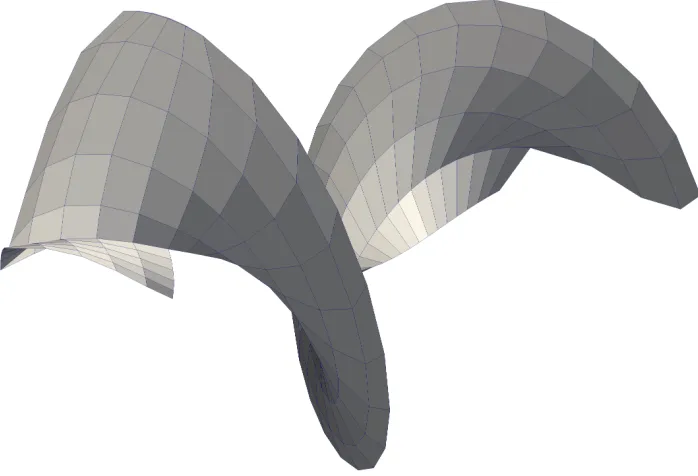
To verify that the implementation of the Kutta condition produces the correct results we will compare the numerical results obtained using the methods presented in this report with 2D results from the analytical solution of flow around a planar, Van de Vooren airfoil [5]. Results will be compared at several angles of attack, illustrating convergence to the analytical solution with respect to panel resolution, and the number of wake panels. Because we will be comparing 3D numerical results with 2D analytical results we will also illustrate the differences between a 2D solution and a 3D solution with a finite wing span, showing convergence to the 2D solution as the span increases.

First, we will examine the convergence of the numerical solution to the analytical results as the the number of panels on the foil increases. Figure 4.6 shows the velocity magnitude on the foil surface (angle of attack = zero) for the 2D analytical solution, plotted with results from coarse, medium, and fine 3D numerical simulations. The coarse, medium, and fine numerical solutions have 10x20, 20x40 and 40x80 panels on the upper and lower faces of the planar foil, respectively. The planar foil in the numerical solutions has a span/chord ratio of approx. 2. The number of streamwise panels used to model the wake for the coarse, medium, and fine discretizations was 40, 80 and 160 respectively. Figure 4.5 shows the body and wake panels for the medium case.

(42)

(43)

Figure 4.7: Velocity Magnitude on surface of foil for a range of span/chord ratios

increases and the geometric approximations improve in these regions of high curvature. However, we also note the failure of the 3D numerical results to converge to the 2D analytical solution due to the 3D eﬀects at the ends of the planar foil body.

The end effects seen in Figure 4.6 are quite small, however as the angle of attack increases 3D end effects become more noticeable. Figure 4.7 shows 3D numerical and 2D analytical results for the same airfoil pictured in figure 4.5, but with an angle of attack of 10 degrees. Numerical results are shown for planar foils with aspect ratios (span/chord) of 2, 4, and 8. The panels on each of these planar foils were the same size as was used in the fine discretization with zero angle of attack and the results were again taken at the spanwise midpoint. Thus figure 4.7 shows us the rate at which the 3D numerical results converge to the 2D analytical results as the foil end effect is moved farther away from the point of interest. Figure 4.7 also shows that those end effects can be significant when comparing the numerical and analytical results.

(44)

Figure 4.8: Velocity Magnitude on surface of foil for 20, 40, and 80 wake panels

(45)

5 Validation

In this chapter we will simulate the ﬂow around a Wageningen B-Series propeller at several advance ratios and compare the thrust and torque predicted by the numerical simulation to the published experimental results for the B-Series [11] [7].

5.1 B-Series Propellers

The Wageningen B-Series propellers were chosen for this validation effort because the exper-imental results are well known to the marine community and because the data was readily available. The series represents a set of propellers with four to seven blades, with a range of expanded area ratios from 0.45 - 1.05 and a range of pitch-diameter ratios from 0.5 - 1.4. Experimentally measured thrust, and torque coefficients have been published for advance ratios from 0.0 - 1.6. Advance ratio, thrust coefficient and torque coefficient are of the forms noted in Chapter 3.

The geometry of the propellers simulated in this report has been recreated from tables of shape parameters published in [11] and [7].

5.2 Propeller Forces

(46)

𝑁𝑆 𝑁𝐶 𝐿

Coarse 5 5 28 Med 7 7 40 Fine 10 10 56 xFine 14 14 80

Table 5.1: Number of panels for the coarse, medium, ﬁne and xﬁne simulations

restrict the usage the numerical model in it’s present state. These diﬀerences may be due to the inviscid and irrotational assumptions in the physical model, however results published by Hoshino [2] for a similar physical model achieved better results.

We also notice that the slope of the numerically predicted 𝐾𝑇 curves is less than that

of the B-Series values; indicating that the numerical method predicts a more constant de-velopment of thrust over variations in advance ratio than is seen in the experimental data. This diﬀerence between the slopes of the numerical and experimental curves could be caused by several of the assumptions made in the physical model, including: the application of the kutta condition at highly loaded blade sections, or the lack of a model for the blade tip vortex.

In ﬁgure 5.6, which plots the 𝐾𝑄 curves, we again see that the slope of the numerically

predicted results is less than that of the experimental results. Torque is highly aﬀected by the induced velocities from the blade tip vortex and the incomplete modeling of that vortex in the method proposed in this report could contribute to the insensitivity of the 𝐾𝑄 curves

to changes in advance ratio.

Also, in figure 5.6 we see that the torque coefficient reduces as the grid resolution in-creases; starting above the experimental results in the Coarse case but falling to below the experimental results in the xFine case; not converging to the experimental results. It is important to note that in the plots of both 𝐾𝑇 and 𝐾𝑄 that the difference between the

numerical values for any two discretizations does not appear to decrease as the panels be-come smaller. This inability to converge, even to results other that the experimental results, could be due to the inadequacies in the physical model mentioned above or to an improper numerical implementation of the continuum equations. In any case, the lack of observed convergence as the panel size is decreased is a problem which must be corrected prior to extensive use of the code.

(47)

Figure 5.1: Panels for coarse simulation, 𝑁𝑆 =𝑁𝐶 = 5

(48)

Figure 5.3: Panels for ﬁne simulation, 𝑁𝑆 =𝑁𝐶 = 10

(49)

(50)

(51)

6 Conclusions

This report describes the governing equation, and boundary conditions for a marine propeller operating in a uniform flow field of inviscid and irrotational fluid and a method is presented by which the velocity and pressure on the blade surface of the propeller can be numerically simulated. The method has been tested on several geometries including a sphere, a planar Van de Vooren airfoil, and a Wageningen B-Series propeller.

The numerical results compared well with the anylitical results for both the sphere and the Van der Vooren airfoil in potential flow, however significant differences were seen when compared to the experimentally measured thrust and torque coefficients for the B-Series propeller. Most troubling is that neither the numerical results for thrust of torque on the B-Series propeller we observed to converge to as the panel size on the computational surfaces was decreased.

Results published by Hoshino [2] show a more favorable comparison with experiemental data, however no grid convergence tests with respect to thrust and torque values were pro-vided in [2]. Other applications of boundary element or panel methods suggests that this type of simulation can provide accurate predictions of the steady thrust and torque on a marine propeller [3].

(52)

Bibliography

[1] J. Hess. Calculation of potential ﬂow about arbitrary three-dimensional lifting bodies. Technical report, Naval Air Systems Command Report, 1972.

[2] T. Hoshino. Hydrodynamic analysis of propellers in steady ﬂow using a surface panel method. Journal of The Society of Naval Architects of Japan, 165:55–70, 1989.

[3] Ching-Yeh Hsin. Development and analysis of panel methods for propellers in unsteady ﬂow. Technical report, Massachusetts Institute of Technology, 1990.

[4] Ching-Yeh Hsin. A panel method for the analysis of the ﬂow around highly skewed propellers. Technical report, Sea Grant College Program, Massachusetts Institute of Technology, 1991.

[5] J. Katz. Low-Speed Aerodynamics: From Wing Theory to Panel Methods. McGraw-Hill, New York, NY, 1991.

[6] Robert Krasny. Computation of vortex sheet roll-up in the treﬀtz plane. Journal of Fluid Mechanics, 184:123–155, 1987.

[7] G. Kuiper. The wageningen propeller series. Technical report, Maritime Research Institute, Netherlands, 1992.

[8] Chang-Sup Lee. Prediction of steady and unsteady performance of marine propellers with or without cavitation by numerical lifting-surface theory. Technical report, Mas-sachusetts Institute of Technology, 1979.

[9] Edward V. Lewis. Principles of Naval Architecture, Volume II. Society of Naval Archi-tects and Marine Engineers, Jersey City, NJ, 1988.

[10] L. Morino. Steady and oscillatory subsonic and supersonic aerodynamics around com-plex conﬁgurations. AIAA Journal, 13:368–374, 1974.

[11] M.W.C Oosterveld. Further computer-analyzed data of the wageningen b-screw series.

Shipbuilding and Marine Engineering Monthly, 22, 1975.

(53)

(54)

Figure A.1: Velocity Magnitude for B5-105, Coarse, 𝑃/𝐷 = 0.8, 𝐽 = 0.3 suction side (left) and pressure side (right)

Figure A.2: 𝐶𝑃 for B5-105, Coarse,𝑃/𝐷 = 0.8,𝐽 = 0.3 suction side (left) and pressure side

(55)

(56)

(57)

(58)

Figure A.9: Velocity Magnitude for B5-105, Medium,𝑃/𝐷 = 0.8,𝐽 = 0.3 suction side (left) and pressure side (right)

Figure A.10: 𝐶𝑃 for B5-105, Medium, 𝑃/𝐷 = 0.8, 𝐽 = 0.3 suction side (left) and pressure

(59)

Figure A.11: Velocity Magnitude for B5-105, Medium, 𝑃/𝐷 = 0.8, 𝐽 = 0.4 suction side (left) and pressure side (right)

(60)

(61)

(62)

Figure A.17: Velocity Magnitude for B5-105, Fine, 𝑃/𝐷 = 0.8, 𝐽 = 0.3 suction side (left) and pressure side (right)

Figure A.18: 𝐶𝑃 for B5-105, Fine, 𝑃/𝐷 = 0.8, 𝐽 = 0.3 suction side (left) and pressure side

(63)

(64)

(65)

(66)

Figure A.25: Velocity Magnitude for B5-105, xFine, 𝑃/𝐷 = 0.8, 𝐽 = 0.3 suction side (left) and pressure side (right)

Figure A.26: 𝐶𝑃 for B5-105, xFine,𝑃/𝐷 = 0.8, 𝐽 = 0.3 suction side (left) and pressure side

(67)

(68)

(69)

(70)

Creation, Verification, and Validation of a Panel Code for the Analysis of Ship Propellers in a Steady, Uniform Wake

ScholarWorks@UNO

ScholarWorks@UNO

Creation, Verification, and Validation of a Panel Code for the

Creation, Verification, and Validation of a Panel Code for the

Analysis of Ship Propellers in a Steady, Uniform Wake

Analysis of Ship Propellers in a Steady, Uniform Wake

Acknowledgments

Contents

List of Figures

List of Tables

List of Symbols

Abstract

1 Introduction

2 The Propeller Flow Problem

2.1

Propeller Geometry and Coordinate System

2.2

Velocity Potential and Boundary Conditions

3 Discretization and Numerical

Method

3.1

Discretization of the Blade, Hub, and Wake

Sur-faces

3.2

First System of Linear Algebraic Equations

3.3

Second System of Linear Algebraic Equations

3.4

Inﬂuence Coeﬃcients

3.5

Satisfaction of the Kutta Condition

3.6

Calculation of Velocity and Pressure on the Blade

Surface

3.7

Calculation of Propeller Forces

4 Veriﬁcation of the Method and

Code

4.1

Sphere in Uniform Flow

4.2

Van de Vooren Airfoil in Uniform Flow

5 Validation

5.1

B-Series Propellers

5.2

Propeller Forces

6 Conclusions

Bibliography

Vita