Kinematic Mapping and Forward Kinematic
Problem of a 5-DOF (3T2R) Parallel
Mechanism with Identical Limb Structures
Mehdi Tale Masouleh
aand Clément Gosselin
aa- Department of Mechanical Engineering, Laval University, 1065 Avenue de la medicine, QC, Canada, G1V0A6. E-mail: [email protected] , and [email protected].
A R T I C L E I N F O A B S T R A C T
Keywords:
5-DOF Parallel Mechanisms Three translation and two independent rotations (3T2R) Study parameters, General and first-order kinematic mapping, Forward Kinematic Problem (FKP), Constant-position workspace.
The main objective of this paper is to study the Euclidean displacement of a 5-DOF parallel mechanism performing three translation and two independent rotations with identical limb structures-recently revealed by performing the type synthesis-in a higher dimensional projective space, rather than relying on classical recipes, such as Cartesian coordinates and Euler angles. In this paper, Study's kinematic mapping is considered which maps the displacements of three-dimensional Euclidean space to points on a quadric, called Study quadric, in a seven-dimensional projective space, P7. The main focus of this contribution is to lay down the essential features of algebraic geometry for our kinematics purposes, where, as case study, a 5-DOF parallel mechanism with identical limb structures is considered. The forward kinematic problem is reviewd and the kinematic mapping is introduced for both general and first-order kinematics, i.e., velocity, which provides some insight into the better understanding of the kinematic behaviour of the mechanisms under study in some particular configurations for the rotation of the platform and also the constant-position workspace.
1. Introduction
The kinematic analysis of parallel mechanisms requires a suitable mathematical framework in order to describe both translation and rotation in a most general way. This can be achieved by resorting to algebraic geometry[1]. The fundamental concept of relating mechanical structures, including parallel mechanisms, with algebraic varieties is called Study's kinematic mapping. This mapping associates to every Euclidean displacement in SE(3),
, a pointc
on a subset of areal projective space
P
7, called the Study quadric7 2 6
P
S
[2, 3]. This subject, i.e., algebraic geometry, occupies a central place in modern mathematics and has multiple conceptual connections with such diverse fields as geometric design, coding theory and mechanisms and robotics. Our interest toward combining and then applying algebraic geometry and Study's kinematic mapping to the kinematic analysis is twofold:1) Using the superabundance of variables which
eliminates the need to resort to trigonometric expressions and produces homogeneous equations;
2) As opposed to formulations based on three-dimensional Euclidean space, algebraic geometry provides a better understanding of the kinematic properties of mechanisms.
Returning to the kinematic analysis of parallel mechanisms, this paper aims first at establishing the relations which allow the general and first-order kinematic mapping of three-dimensional Euclidean space to the Study parameters and then the Forward Kinematic Problem (FKP) for the topologically symmetric 5-DOF parallel mechanisms performing a specific motion patterns which are described in what follows. In general, 5-DOF parallel mechanisms are a class of parallel mechanisms with reduced degrees of freedom which, according to their mobility, fall into three classes [4]:
1) Three translational and two rotational freedoms (3T2R);
freedoms (3R2
T
p):a) (3R2
T
pi) with instantaneous planar motion; b) (3R2T
pf ) with fixed planar motion;3) Three rotational and two spherical translational
freedoms (3R2
T
s).For the 5-DOF parallel mechanisms, this paper deals with the first one, i.e., the one performing 3T2R motion pattern. Geometrically, the 3T2R motion can be made equivalent to guiding a combination of a directed line and a point on it. Accordingly, the 3T2R mechanisms can be used in a wide range of applications for a
point-line combination including, among others, 5-axis machine tools [5, 6], welding and conical spray-gun. In medical applications that require at the same time mobility, compactness and accuracy around a functional point, 5-DOF parallel mechanisms can be regarded as a very promising solution [7].
Based on the results obtained from type synthesis and the recent study conducted in [8-11], two kinematic arrangements may be of practical interest for symmetric 5-DOF parallel mechanisms (3T2R), namely: 5-PRUR [10] and 5-RPUR [8, 9]. In this paper, as a case study, we consider 5-RPUR. Here and throughout this paper, P stands for a prismatic joint R for a revolute joint and U for an universal joint. To distinguish the actuated joint from a non-actuated one, which is referred to as passive
joint, the actuated one is underlined, for instance P. It should be noted that the FKP of 5-DOF parallel mechanisms (3T2R) was solved in [10, 12]. The latter study revealed that this kind of mechanisms have up to 1680 finite solutions and for a simplified design a univariate expression of degree 220 was obtained. Of even more importance, for a general design 208 real solutions were found for the FKP. In the latter studies the emphasis was placed on solving the FKP of a 5-PRUR parallel mechanism, by means of Study's kinematic mapping [10, 12-16].
The remainder of this paper is organized as follows. First, to lay down the essential concept for the projective space, Study's kinematic mapping is given. Then the architecture of the 5-RPUR parallel mechanism is reviewed. The constraint and FKP expressions are presented based on the results of some recent studies. Then, the general kinematic mapping is introduced which makes it possible to find the position and orientation (pose) of the mobile platform by having in place its corresponding information in the projective space, i.e., the Study's parameters, and vice versa. The first-order kinematic constraint of the 5-DOF parallel mechanism under study is obtained by means of Study's parameters and different sets are represented which fully describe Study's parameters and their corresponding rate changes. Moreover, the regularity of the mapping obtained is examined and some particular configurations are treated in detail. Then, the constant-position workspace is investigated using the relations given for the kinematic mapping.
2. Study’s Kinematic Mapping
The Euclidean group is the group of transformations of
the vector space
R
ne that preserve the Euclidean metric. This group is denoted as SE(3) forn
e=
3
which represents the complete rigid body motion in space. An Euclidean displacement is a mapping:
, ,
:R3R3 xAxa
(1) whereA
is a proper orthogonal three by three matrix.The mapping of SE(3) onto the points of
S
62
P
7iscalled the kinematic mapping. In turn, Study's kinematic mapping is a mapping of an element
of the Euclidean displacement group SE(3) into a7-dimensional projective space,
P
7 [3]. The homogeneous coordinates of a point inP
7 are given bys
=
(
x
0:
x
1:
x
2:
x
3:
y
0:
y
1:
y
2:
y
3)
. Thekinematic pre-image of
s
is the displacement
described by the transformation matrix:,
) 2( ) 2(
) 2( )
2(
) 2( ) 2(
0 0
0
1 =
2 3 2 2 2 1 2 0 1 0 3 2 2 0 3 1
1 0 3 2 2 3 2 2 2 1 2 0 3 0 2 1
2 0 3 1 3 0 2 1 2 3 2 2 2 1 2 0
x x x x x x x x x x x x r
x x x x x x x x x x x x q
x x x x x x x x x x x x p H
H
Ω
(2)
where
). 2(
=
), 2(
=
), 2(
= , =
0 3 1 2 2 1 3 0
1 3 0 2 3 1 2 0
2 3 3 2 0 1 1 0 2
3 2 2 2 1 2 0
y x y x y x y x r
y x y x y x y x q
y x y x y x y x p x x x x H
(3)
Note that the lower right three by three sub-matrix is a proper orthogonal matrix if:
0,
=
3 3 2 2 1 1 0
0
y
x
y
x
y
x
y
x
(4) and not allx
i are zero. If these conditions are fulfilledT
y
x
:
:
)
(
0
3 are called Study parameters of the displacement
. Equation (4) defines a quadric, theso-called Study quadric,
S
62, which lies on a sevendimensional kinematic space,
P
7. Thus the range of thekinematic mapping is the Study quadric,
S
62, minus thethree dimensional subspace defined by: 0.
= = = =
:x0 x1 x2 x3
Ex (5)
2 6
S
is called Study quadric andE
x is the exceptionalor absolute generator. One can normalize the parameters such that
H
=
1
, then the coordinatex
0 representsthe cosine of the half rotation angle. Note that there are other possibilities to normalize.
Reaching this step, the prime concern is with obtaining the correspondence between the Study parameters and the component of a given matrix which represents the motion of a rigid body. Let
A
=
[
a
]
i,j=0,4 be thisgeneral matrix which can be obtained using the D-H convention. This mapping consists in re-parametrization of the Euclidean displacements using algebraic parameters. It should be noted that the quadruple
)
:
:
:
(
=
x
0x
1x
2x
3parameters and the best way, i.e., free of parametrization singularity, of computing the Euler parameters was already known to Study [2]. He demonstrated that for any Euclidean transformation, in this case
A
, the homogeneous quadruplex
=
(
x
0:
x
1:
x
2:
x
3)
can beobtained from at least one of the following proportions:
33 22 11 32 23 13 31 12 21
32 23 33 22 11 21 12 31 13
13 31 21 12 33 22 11 23 32
12 21 31 13 23 32 33 22 11 00
3 2 1 0
1
:
:
:
=
:
1
:
:
=
:
:
1
:
=
:
:
:
=
:
:
:
a
a
a
a
a
a
a
a
a
a
a
a
a
a
a
a
a
a
a
a
a
a
a
a
a
a
a
a
a
a
a
a
a
a
a
a
a
x
x
x
x
(6)
It can be shown that all four proportions are valid representations [15]. In fact, each proportion is not singular-free per se. However, the set as a whole is free of any parametrization singularity. The singularity for one proportion occurs when the quadruple vanishes,
0)
:
0
:
0
:
(0
=
x
, i.e.,x
E
x. In this case, one shoulduse the above proportions until a non-vanishing quadruple is obtained. The reason for which this set of representation is singular-free is that it is impossible that all the proportions vanish simultaneously. In the case that the first three proportions go to zero we resort to the last proportion which yields
x
=
(0
:
0
:
0
:
1)
. The four remaining Study parameters)
:
:
:
(
=
y
0y
1y
2y
3y
can be computed from:. =
2 , =
2
, =
2 ,
= 2
2 21 1 31 0 41 3 3 21 1 41 0 31 2
3 31 2 41 0 21 1 3 41 2 31 1 21 0
x a x a x a y x a x a x a y
x a x a x a y x a x a x a y
(7)
3. 5-RPUR Parallel Mechanisms
A. Architecture Review and Kinematic Modelling
Figures 1(a) and 1(b) provide respectively a
representation of a RPUR limb and a 5-DOF parallel
mechanism that can be used to produce all three
translational DOFs plus two independent rotational
DOFs (3T2R). The Cartesian coordinates of the
end-effector are noted
(
x
,
y
,
z
,
,
)
. In the latternotation, p=[x,y,z]T represents the translational DOFs, a position vector of a chosen point on the
end-effector, with respect to the fixed frame
O
, asshown in Fig. 1(a), while
(
,
)
stand for theorientation DOFs around axes
y
(
e
1)
andx
,respectively. The rotation sequence between the desired
orientation of the platform and angles
and
is thefirst rotation, of angle
, aboute
2 followed by asecond rotation of angle
aboute
1.(a)One limb (b) CAD model
Fig.1a) Kinematic arrangement for a RPUR limb and (b) a CAD model for a 5-RPUR parallel mechanism.
Based on the latter rotation sequence the rotation matrix can be expressed as follows:
. cos cos cos sin sin
sin cos
0
sin cos sin sin cos =
Q (8)
Vectors
e
1 ande
2 are unit vectors respectively alongthe first and last revolute joints of each leg. They are the same for all leg, by construction. We define respectively
T
z
y
x
,
,
]
[
=
p
andω
=
[
x,
y,
z]
T as the reference pointp
of the platform velocity and the angular velocity of the mobile platform.This mechanism consists of an end-effector which is linked by 5 identical limbs of the RPUR type to a base. The input of the mechanism is provided by the five linear prismatic actuators. From the type synthesis presented in [17], the geometric characteristics associated with the components of each leg are as follows: The five revolute joints attached to the platform (the last R joint in each of the legs) have parallel axes, the five revolute joints attached to the base have parallel axes, the first two revolute joints of each leg have parallel axes and the last two revolute joints of each leg have parallel axes. It should be noted that the second and third revolute joints in each leg are built with intersecting and perpendicular axes and are thus assimilated to U joints. Further results regarding the kinematic properties, such as the solution of the IKP, FKP and the determination of the constant-orientation workspace can be found in [10, 12, 18].
B. Forward Kinematic Problem
The FKP of the 5-RPUR has been extensively studied in [10, 12] which revealed that the forward kinematic expression,
F
p, of the principal limb, a limb for which
( )
=0. 16 ) 8( ) 8( = ) ( 2 2 1 2 2 2 2 2 2 3 2 0 2 1 2 2 3 0 3 0 1 2 2 1 2 2 2 2 2 1 1 2 2 x x l y y y y x y y x x y x y l x y x y l s F p p p p p p p (9)
0.
=
=
2 3 2 2 2 1 20
x
x
x
x
C
(10) Moreover, from the latter studies, 1680 finite solutions was found for the FKP where for a given design and input parameters 208 real solutions was reported (This is not an upper bound for the number of the real solutions). However, there are still some gaps for the general and first-order kinematic mapping of such mechanisms which is the subject of the following sections.C. Mapping between Study Parameters and Three-dimensional Euclidean Space
In this section, we attempt to set up correspondences between the Study parameters and the three dimensional Euclidean space and vice versa. These transformations can be used to convert the solutions obtained for the FKP which are explored in projective space, i.e., Study parameters, in order to ensure their validity and to provide a physical sense to the solutions.
1) Cartesian representation of Study’s parameters:
Mathematically, the mapping from an element of
P
7,7
P
s
, into a three-dimensional real vector space, called Euclidean three space, SE(3), is defined as:,
)
(
),
(
(3),
:
P
7SE
m
m
R
5m
s
s
ss
ss
(11)where
R
5, stands for the five-dimensional real array space representing the three translations and two permitted rotational DOFs. The first step is to compute the rotational DOFs(
,
)
. To this end, the lower threeby three sub matrix of
Ω
, Now, the inspection of the components ofQ
and those ofΩ
t leads to a uniquesolution for
and
, namely:),
,
2(
arctan
=
x
1x
3
x
0x
2x
2x
3
x
0x
1
(12)).
,
2(
arctan
=
x
2x
3
x
0x
1x
1x
3
x
0x
2
(13)To compute the position of the platform,
p
=
[
x
,
y
,
z
]
T, for a given set of
x
=
[
x
0:
x
1:
x
2:
x
3]
obtained above,one should use the following [15]:
.
=
2
,
=
2
,
=
2
,
=
2
2 1 0 3 3 1 0 2 3 2 0 1 3 2 1 0x
x
y
x
z
x
y
x
x
z
x
y
x
y
y
x
z
x
x
x
y
z
x
y
x
x
x
y
(14)One could consider any three equations in order to obtain a unique set of solutions for
(
x
,
y
,
z
)
for a givens
. By considering the first four equations it results that the determinant of this system of equations is:).
(
322 2 2 1 2 0
3
x
x
x
x
x
(15) For the considered system of equations, oncex
3=
0
the system of equations degenerates. Using the fact that this system of equation is overdetermined, one can establish another system of equations which avoids this singular condition. For instance in the previous case when
x
3=
0
one could consider a system of equationsin which the first equation is replaced by the fourth one and the determinant becomes:
).
(
2 3 2 2 2 1 2 00
x
x
x
x
x
(16)It follows that when
x
3=
0
then2
2
=
0
x
andthe system of equations is of full rank. Once the latter system of equations is solved for
(
x
,
y
,
z
)
the position of the platform,p
, with respect to the base frame presented in Fig. 1(a) becomes:.
]
,
,
[
=
y
z
x
Tp
(17) Following the same procedure, one can transform the vectors describing the geometry of the base and platform, written in terms of Study's parameters,]
,
,
[
=
1i 6i ib
b
b
andm
i=
[
m
1i,
,
m
6i]
,respectively, into the vectors describing them in the Cartesian coordinates,
r
i ands
'
i (See Fig. 1).Skipping the mathematical derivations one obtains: . ] 2 , 2 , 2 [ = , ] 2 , 2 , 2 [
= 6 7 5 7 5 6
T i i i i T i i i
i b b b s' m m m
r (18)
It is recalled that due to the parallelism of the axes attached to the base and platform, one has:
0
=
=
=
=
2 3 41i
b
ib
ib
ib
and0
=
=
=
=
2 3 41i
m
im
im
im
.2) Representation of Study’s Parameters in Terms of Three-dimensional Euclidean Space:Mathematically, the mapping from an element of SE(3),
R
5, into seven-dimensional space,P
7, is defined as:).
)
(
(
,
(3)
:
7
k
s
k
SE
P
m
m
(19)The mapping from Cartesian space to Study's parameters requires further mathematical manipulations. Without loss of generality, assume the homogeneous condition to be:
1
=
=
02 12 22 32 2 3 0 =x
x
x
x
x
i i
(20) From Eqs. (12) and (13) it follows that:.
cos
sin
=
4
,
sin
cos
=
4
x
1x
3
x
2x
3
(21)Squaring both sides of the above expressions and adding them results in:
).
(
sin
2
2
=
)
(
16
2 2 2 1 23
x
x
x
(22)Combing the homogeneous and constraint equation, Eq. (10), one has:
,
2
1
=
,
2
1
=
02 322 2 2
1
x
x
x
x
(23)where one can obtain the following for and
x
0 and3
x
: . 2 ) ( sin 1 1) ( = , 2 ) ( sin 1 1) ( = 2 0 1 3 xx (24)
In the above, 1={0,1} and 2={0,1} stand for the two distinct solutions. As it can be observed from the above, this mapping admits two distinct solutions for
3
Cartesian space. These two distinct solutions can be classified as follows: (a)
>
0
then
1=
2 and(b)
0
then
1
2. Handling the values for0
x
andx
3 and substituting into Eq. (12) leads to:,
=
sin
,
=
cos
x
1x
3
x
0x
2
x
2x
3
x
0x
1 (25) which, once solved forx
1 andx
2 yield:). cos sin
( = ), sin cos (
= 3 0 2 3 0
1 x
x
x x
x
x (26)
The transformation for the fixed parameters
r
i ands
'
i, vector representing respectively the geometry of the base and platform as depicted in Fig. 1, can be readily obtained using Eq. (18). The rotational parameters, i.e,
x
andy
=
[
y
0:
y
1:
y
2:
y
3]
can be found by backsubstitution into Eq. (14).
Thus from above it follows that the mapping from the Study parameters to the Cartesian space is one to one and the converse, i.e., from Cartesian space to Study's parameters is two to one. This is called double covering of the Euclidean displacement group SE(3). For example: The dual quaternions are a double covering of SE(3).
D. First-order Kinematic Mapping and Different sets in P 7for describing
x
x
We direct our attention to a formulation based on the projective space which leads to define different sets in order to fully determine the Study parameters and their corresponding time rate of change. Combining the homogeneous and constraint condition leads to:
.
2
1
=
,
2
1
=
12 222 3 2
0
x
x
x
x
(27)Differentiating the above with respect to time results in :
0.
=
0,
=
1 1 2 23 3 0
0
x
x
x
x
x
x
x
x
(28) Then, combining the above with Eqs. (27) leads to the following system of equations:
2
1
=
0
=
,
2
1
=
0
=
2 2 2 1
2 2 1 1 2
3 2 0
3 3 0 0
x
x
x
x
x
x
x
x
x
x
x
x
(29)
The above allows to conclude that prescribing
]
:
:
:
[
=
x
0x
1x
2x
3
x
results in two solutions tox
:
2 2 2 1 1 2
2 2 2 1 2 1
2 3 2 0 0 3
2 3 2 0 3 0
2 2 =
2 2 =
2 2 =
2 2 =
x x
x x
x x
x x
x x
x x
x x
x x
(30)
From Eq. (29), one can define different sets to fully determine
x
x
=
[
x
:
x
]
. In order to obtain these sets, wedefine
X
p1 andX
p2 respectively as the set ofparameters which allow to solve the first and second system of equations presented in Eq. (29) as follows:
[ , ],[ , ],[ , ],[ , ]
,= 0 0 0 3 3 0 3 3
1 x x x x x x x x
Xp (31)
[
,
],
[
,
],
[
,
],
[
,
]
.
=
1 1 1 2 2 1 2 12
x
x
x
x
x
x
x
x
X
p
(32)Consequently, a set, called
X
p , which is thetwo-by-two combination of components of
X
p1 and2 p
X
allows to fully determinex
x
and is formulated as follows:]. , , , [ ) (
= 0 1 2 3
2 2
1 X x x x x
X
Xp p p (33)
Thus it can be inferred that 21 different sets exist in order to fully determine
x
andx
. It follows that the rotation and angular velocity of the mobile platform can be fully prescribed either by prescribing all the time derivatives of the Study parameters,x
, or by a combination of some Study parameters and their timederivatives,
(
X
p1
X
p2)
2.E. First-order Kinematic Mapping for the Angular Velocity
Here, we direct our attention to the mapping of the first-order kinematics from the time derivative of the Study parameters,
x
andy
=
[
y
0,
y
1,
y
2,
y
3]
, to thevelocity and angular velocity
p
=
[
x
,
y
,
z
]
T and
. 1) Mapping of the Time Derivative of Three-dimensional Euclidean Space to Study’s Parameters:Referring to Eq. (24) and upon differentiating with respect to time, and skipping mathematical derivations, one has:
). ( cos 8 1) ( =
3 1
3
x
x (34)
As it can be observed, the above fails to result in a solution for
x
3 when1
sin
(
)
=
0
which in the projective space corresponds to a configuration for whichx
3=
0
. In order to avoid such a configurationthe corresponding value for
cos
(
)
should be found by referring to Eq. (22):. 2 1 2 2 = ) (
cos 2
3
3 x
x
(35) Upon substituting the above into Eq. (34) and replacing the corresponding expression found for
x
3 in Eq. (24) leads to:, ) ( sin 1 4 1) (
= 1
3
x (36)
which is obviously singularity-free. Following the same reasoning it follows that:
. ) ( sin 1 4 1) (
= 1
0
x (37)
, cos sin
sin cos
= 3 3 0 0
1 x
x
x
x
x (38)
.
sin
cos
cos
sin
=
3 3 0 02
x
x
x
x
x
(39)It should be noted in the above that one should use respectively Eqs. (36) and (37) for the mapping of
x
3and
x
0 and Eq. (24) forx
3 andx
0.2) Mapping of the Time Derivative of the Study Parameters to the Three-dimensional Euclidean Space:
From Eq. (12) it follows that: ), (
=
sin x1x3 x1x3 x0x2 x2x2
(40)).
(
=
cos
x
2x
3x
2x
3x
0x
1x
0x
1
(41)Squaring both sides and then adding leads to:
( ) ( )
.4
= 2
1 0 1 0 3 2 3 2 2 2 2 2 0 3 1 3 1
2 xx xx xx xx xx xx xx xx
(42)A similar approach yields to the following for
:
(
)
(
)
.
4
=
13 13 02 0222 1 0 1 0 3 2 3 2
2
x
x
x
x
x
x
x
x
x
x
x
x
x
x
x
x
(43)where, finally, upon skipping some mathematical manipulations, one has:
,2
= 32
2 0 2 2 2
1 x x x
x
(44)
.2
= 2
3 2 0 2 2 2
1 x x x
x
(45)F. First-order Kinematic Mapping for the Point Velocity
The relations allowing the mapping of angular velocity from the projective space into the three-dimensional Euclidean space, and vice versa, can be readily extended to obtain the mapping for the translational velocity. This can be done by differentiating Eq. (14) with respect of time.
G. From three-dimensional Euclidean Space to Study’s Parameters
In this case the pose of the platform,
(x,
y,
z,
,
θ
)
andthe time rate of change of its coordinates,
(
x
,
y
,
z
,
,
)
are given. Upon differentiating Eq. (14) with respect to time one could readily find
y
.H. From Study’s Parameters to the Three-dimensional Euclidean Space
In this case the time derivative of Eq. (14) with respect to time should be solved for
(
x
,
y
,
z
)
by having in hands
,x
andy
. Finally, based on Eq. (17), it follows that:.
]
,
,
[
=
y
z
x
T
p
(46) It should be noted that in the case that the above system of equation is rank deficient one should proceed as explained in section 2.3.1. As a consequence the above mappings are both singularity-free.4. Some Applications of Kinematic Mapping Generally, in the context of parallel mechanisms, the Study kinematic mapping is used to investigate the FKP and due to its mathematical complexities, initiated several researches both in mathematics and mechanics.
From the begining of this section some insight was given for the FKP of the 5-DOF parallel mechanism under study where for the next mechanism more details will be provided. In what follows, we resort to Study kinematic mapping in order to first explore some kinematic properties of the 5-DOF parallel mechanism under study for some particular rotational configurations, which cannot be obtained by entailing the study in three-dimensional Euclidean space. Then, a subset of workspace, called the constant-position workspace, is elaborated.
A. Particular Configurations for the Kinematic Mapping of 5-RPUR Parallel Mechanisms
As stated before, the sets belonging to
X
p may fail to fully determinex
x
. These configurations are treatedhereafter for
[
x
0,
x
1,
x
2,
x
3]
and the set belonging to2 2
1
)
(
X
p
X
p . It should be noted that these configurations should not be interpreted as singular configurations and that there are configurations which admitinfinitely many solutions.
1) Particular configuration for
[
x
0,
x
1,
x
2,
x
3]
:In general for a given
x
, which stands for the angular velocity of the platform, one can readily determine its correspondingx
. In fact, ifx
is prescribed then one could readily findx
from Eq.(30) and also
and
respectively from Eqs. (44) and (45). Then havingx
by using Eqs. (12)and (13) leads to obtaining
and
. This means thatx
is the central quantity of the mapping. This issue is depicted in Fig. 2. As it can be observed from the latter tree-model having in placex
allows to find
x
,(
,
)
and(
,
)
. As mentioned above there are some configurations for which the mapping would have infinitely many solutions. Inspecting Eq. (30) it follows that in the following case the mechanism would have infinitely many solutions for the rotational DOF:0,
=
0]
[0,
=
]
,
[
x
0x
3
(47)0,
=
0]
[0,
=
(48)0.
=
=
0]
0,
0,
[0,
=
(49)
Fig.2Schematic representation of the mapping of the rotational parameters.
angular velocity as given above, can be produced for any of the orientations of the mechanism.
2. Particular configuration for
(
X
p1
X
p2)
2:In this case, for a configuration in which one of the Study parameters becomes zero, then it would impossible to fully determine
x
. Let's considerrespectively the first and third component of
X
p1 and 2p
X
which results in[
x
0,
x
2,
x
0,
x
2]
. In the case that0
=
0
x
thenx
0, and as consequencex
, may have infinitely many solutions. These configurations and their influences in both projective space and three dimensional Euclidean space can be summarized as follows:,
2
=
0,
=
0
=
30
x
x
(50)
,
2
=
0,
=
0
=
21
x
x
(51)
,
2
=
0,
=
0
=
12
x
x
(52).
2
=
0,
=
0
=
03
x
x
(53)The above configurations can be interpreted as follows: the mechanism is able to perform any angular velocity for
and
.B. Constant-position Workspace
This subset of workspace consists of the feasible orientations of the platform for a prescribed position of the platform. Usually, it is very cumbersome to assess geometrically such a workspace and it is preferable to perform this analysis using numerical methods. In three-dimensional Euclidean space, this can be formulated as obtaining intervals for
and
for which all the actuators satisfy the stroke limits. It should be noted that the constant-orientation workspace was investigated in detail [19] where Bohemian domes came up for the vertex space.
Fig.3Constant-position workspace for a 5-RPUR parallel mechanism. The grey zones are not permitted.
It should be noted that the analysis of the constant-position workspace in three-dimensional Euclidean space is a delicate task. Figure 3 represents the constant-position workspace for a 5-RPUR parallel mechanism for a given position which is plotted in a two-dimensional Cartesian coordinates.
It would be more advantageous and enlightening to explore such a problem in seven-dimensional kinematic space and by resorting to the kinematic mapping presented previously it can be readily converted into three-dimensional Euclidean space. Moreover, this approach results in a meaningful representation of the orientation workspace, which is an angular travel around a circle, Fig. 4. Usually, the results of constant-orientation workspace are plotted in a Cartesian space which is more meaningful for the position purpose and few appropriate environments have been reported in the literature for the constant-position workspace, for instance the study elaborated in [20] for spatial parallel mechanisms. To follow the proposed approach, the given position of the platform should be expressed in terms of Study parameters. This can be achieved using Eq. (14) which is recalled here:
. =
2 , =
2
, =
2 ,
= 2
2 1 0 3 3 1 0 2
3 2 0 1 3 2 1 0
x x y x z x y x x z x y x y
y x z x x x y z x y x x x y
(54)
For a given position vector
(
x
,
y
,
z
)
and upon substitutingthe
y
obtained from the above relations intoF
p, one obtains an expression which is a function of onlyx
andp
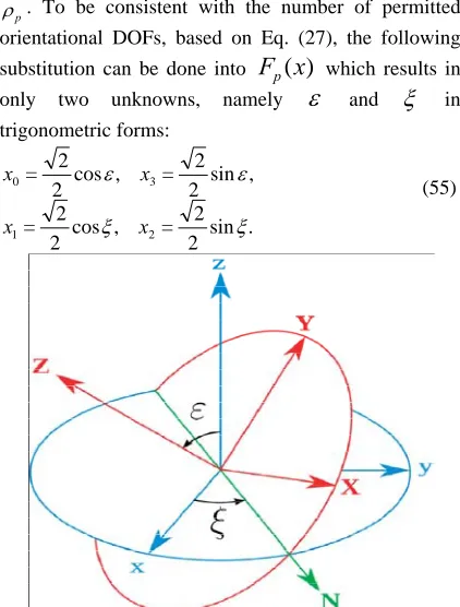
. To be consistent with the number of permitted orientational DOFs, based on Eq. (27), the following substitution can be done into
F
p(
x
)
which results inonly two unknowns, namely
and
intrigonometric forms:
. sin 2
2 = , cos 2
2 =
, sin 2
2 = , cos 2
2 =
2 1
3 0
x x
x x
(55)
It should be noted that the obtained solutions for
and
cannot be plotted along the two constraint circles since they are not decoupled. To do so, we use a spherical representation which is notationally depicted in Fig. 4. Then by applying the tan-half substitution for 2 tan
=
t and
2 tan
=
t , one obtains:
0. = ) , , ( t t p p
OF
(56)
The above corresponds to the principal limb and applying the same procedure explained in [12] for obtaining the forward kinematic expressions for other limbs, one can readily find the corresponding expressions for the other four limbs:
,5. 2, = 0, = ) , ,
( j
Fj t t j
O (57)
In what concerns the degree of the above expressions, it follows that the power of
p and
jare all even numbers. Thus by applying a simple
substitution of the type
p2=
p and
2j=
j , pO
F
can be reduced to a second degree polynomial
expression. Thus one should solve Eqs. (56) and (57) with respect to the extension of the actuators in order to find the possible angular travels, i.e.,
t and
t whichcan be readily transformed to
and
. Figure 5 represents an example for the constant-position workspace where the workspace is the whole surface of the sphere except the regions which do not include the arrows.
Fig.5: Constant-position workspace for a general 5-RPUR parallel mechanism.
5. Conclusions
This paper investigated the kinematic mapping of the constraint parameters and the forward kinematic problem of a 5-DOF parallel mechanism with identical limb structures performing a 3T2R motion pattern. The mappings from the projective space, Study parameters, to the three-dimensional Euclidean space, and vice versa, were given. Following a similar approach, the first-order kinematics, i.e., velocity mapping was elaborated. By combining the results obtained for both general and first-order kinematic mapping some particular configurations were obtained and physical interpretations were associated to them which would
have been difficult without resorting to such a mapping. Moreover, the constant-position workspace for the 5-DOF parallel mechanism under study was investigated. Ongoing work includes the optimum synthesis of the mechanism under study.
Acklowledgment
The authors would like to acknowledge the financial support of the Natural Sciences and Engineering Research Council of Canada (NSERC) as well as the Canada Research Chair program.
References
[1] D. A. Cox, J. B. Little, and D. O’shea, Using Algebraic Geometry. Springer Verlag, 2005.
[2] E. Study, “ Von den Bewegungen und Umlegungen,”
Math. Ann., vol. 39, pp. 441–566, 1891.
[3] M. L. Husty and H.-P. Schrocker,¨ “Algebraic Geometry and Kinematics.” Nonlinear Computational Geometry edited by Emiris, I. Z., Sottile F. and Theobald T., 2007, pp. 85–106.
[4] X. Kong and C. Gosselin, Type Synthesis of Parallel Mechanisms. Springer, Heidelberg, 2007, vol. 33. [5] “Parallelmic, http://www.parallemic.org/.”
[6] F. Gao, B. Peng, H. Zhao, and W. Li, “A Novel 5-DOF Fully Parallel Kinematic Machine Tool,” The
International Journal of Advanced Manufacturing Technology, vol. 31, no. 1, pp. 201–207, 2006.
[7] O. Piccin, B. Bayle, B. Maurin, and M. de Mathelin, “Kinematic Modeling of a 5-DOF Parallel Mechanism for Semi-Spherical Workspace,” Mechanism and Machine Theory, vol. 44, no. 8, pp. 1485–1496, 2009.
[8] C. Gosselin, M. Tale Masouleh, V. Duchaine, P. L. Richard, S. Foucault, and X. Kong, “Parallel Mechanisms of the Multipteron Family: Kinematic Architectures and Benchmarking,” in IEEE International Conference on
Robotics and Automation, Roma, Italy, 10-14 April 2007, pp. 555–560.
[9] M. Tale Masouleh and C. Gosselin, “Singularity Analysis of 5-RPRRR Parallel Mechanisms via Grassmann Line Geometry,” in Proceedings of the
2009 ASME Design Engineering Technical Conferences, DETC2009-86261.
[10]M. Tale Masouleh, M. Husty, and C. Gosselin, “Forward Kinematic Problem of 5-PRUR Parallel Mechanisms Using Study Parameters,” in Advances in Robot
Kinematics: Motion in Man and Machine. Springer, 2010, pp. 211–221.
[11]M. Tale Masouleh, M. H. Saadatzi, C. Gosselin, and H. D. Taghirad, “A Geometric Constructive Approach for the Workspace Analysis of Symmetrical 5-PRUR Parallel Mechanisms (3T2R),” in Proceedings of the 2010 ASME
Design Engineering Technical Conferences, DETC2010-28509.
[12]M. Tale Masouleh, M. Husty, and C. Gosselin, “A General Methodology for the Forward Kinematic Problem of Symmetrical Parallel Mechanisms and Application to 5-PRUR parallel mechanisms (3T2R),” in
Proceedings of the 2010 ASME Design Engineering Technical Conferences, DETC2010-28222.
[13]M. L. Husty, “An Algorithm for Solving the Direct Kinematics of General Stewart-Gough Platforms,”
365–379, 1996.
[14]D. R. Walter, M. Husty, and M. Pfurner, “The SNU-3UPU Parallel Robot from a Theoretical Viewpoint ,” in Fundamental Issues and Future Research Directions for Parallel Mechanisms and Manipulators, Montpellier, France, 21–22 September 2008, pp. 151–158.
[15]K. Brunnthaler, “Synthesis of 4R Linkages Using Kinematic Mapping,” Ph.D. dissertation, Institute for Basic Sciences in Engineering, Unit Geometry and CAD, Innsbruck, Austria, December 2006.
[16]M. Tale Masouleh, C. Gosselin, M. H. Saadatzi, and H. D. Taghirad, “Forward Kinematic Problem and Constant Orientation Workspace of 5-RPRRR (3T2R) Parallel Mechanisms,” in 18th Iranian Conference on Electrical
Engineering (ICEE). IEEE, 2010, pp. 668–673. [17]X. Kong and C. Gosselin, “Type Synthesis of 5-DOF
Parallel Manipulators Based on Screw Theory,” Journal
of Robotic Systems, vol. 22, no. 10, pp. 535–547, 2005. [18]M. Tale Masouleh and C. Gosselin, “Kinematic
Analysis and Singularity Representation of 5-RPRRR Parallel Mechanisms,” in Fundamental Issues and Future Research Directions for Parallel Mechanisms and Manipulators, Montpellier, France, 21–22 September 2008, pp. 79–90.
[19]M. Tale Masouleh, C. Gosselin, M. H. Saadatzi, X. Kong, and H. D. Taghirad, “Kinematic Analysis of 5-RPUR (3T2R) Parallel Mechanisms,” Meccanica,vol. 46, no. 1, pp. 131–146, 2011.
[20] I. A. Bonev, “Geometric Analysis of Parallel Mechanisms,” Ph.D. dissertation, Laval University.
Biography of Authors
Mehdi Tale Masouleh received the B. Eng. and Ph.D. degrees in Mechanical engineering from the Laval University, Québec, Canada, in 2006 and 2010, respectively. Currently, he is a Postdoctorall Fellow under the supervision of Prof. Gosselin in the Robotic Laboratory of Laval University. His research interests are kinematics studies and design of serial and parallel robotic systems with a particular emphasis on the application of algebraic geometry in kinematic modeling of mechanical structures.
Clément Gosselin received the B. Eng. degree in Mechanical Engineering from the Université de
Sherbrooke, Québec, Canada, in 1985, at which time he was presented with the Gold Medal of the Governor General of Canada. He then completed a Ph.D. at McGill University, Montréal, Québec, Canada and received the D. W. Ambridge Award from McGill for the best thesis of the year in Physical Sciences and Engineering in 1988. In 1989 he was appointed by the Department of Mechanical Engineering at Université Laval, Québec where he is now a Full Professor since 1997. He is currently holding a Canada Research Chair on Robotics and Mechatronics since January 2001.