of peer-reviewed research and commentary in the population sciences published by the Max Planck Institute for Demographic Research Konrad-Zuse Str. 1, D-18057 Rostock · GERMANY www.demographic-research.org
DEMOGRAPHIC RESEARCH
VOLUME 13, ARTICLE 16, PAGES 389-414
PUBLISHED 17 NOVEMBER 2005
http://www.demographic-research.org/Volumes/Vol13/16/ DOI: 10.4054/DemRes.2005.13.16
Research Article
Estimates of mortality and population
changes in England and Wales
over the two World Wars
Dmitri Jdanov
Evgeny Andreev
Domantas Jasilionis
Vladimir M. Shkolnikov
This article is part of Demographic Research Special Collection 4, “Human Mortality over Age, Time, Sex, and Place: The 1st HMD Symposium”.
1 Introduction 390
2 Data and Methods 392
2.1 The First World War (1914-1918) 392 2.2 The Second World War (1939-1945) 394
2.3 Methods 396
3 Model 397
3.1 Population flows 397
3.2 Assumptions 399
3.3 Parameterized model 400
3.4 The minimization functional 402
4 Results 404
4.1 The First World War 405
4.2 The Second World War 408
5 Conclusion 409
6 Acknowledgements 411
Estimates of mortality and population changes in England and Wales
over the two World Wars
Dmitri Jdanov1, Evgeny Andreev2, Domantas Jasilionis1,
Vladimir M. Shkolnikov1
Abstract
Almost one million soldiers from England and Wales died during the First and Second World War whilst serving in the British Armed Forces. Although many articles and books have been published that commemorate the military efforts of the British Armed Forces, data on the demographic aspects of British army losses remain fragmentary. Official population statistics on England and Wales have provided continuous series on the civilian population, including mortality and fertility over the two war periods. The combatant population and combatant mortality have not been incorporated in the official statistics, which shows large out-migration at the beginning and large in-migration towards the end of the war periods. In order to estimate the dynamics of the total population and its excess mortality, we introduce in this paper a model of population flows and mortality in times of war operations. The model can be applied to a detailed reconstruction of war losses, using various shapes of the input data. This enables us to arrive at detailed estimates of war-related losses in England and Wales during the two world wars. Our results agree with elements of data provided by prior studies.
This article is part of Demographic Research Special Collection 4,
“Human Mortality over Age, Time, Sex, and Place: The 1stHMD Symposium”. Please see Volume 13, Publications 13-10 through 13-20.
1. Introduction
Reliable statistics covering the whole population of England and Wales date back to the beginning of the 19th century. Only a few countries in the world have longer continuous data series on their population. The historical data on England and Wales have a number of unresolved problems, however. In this paper, we address one of them: the incomplete-ness of population figures for the periods covering the two world wars.
Data on the British population for these periods are split into two separate series. As to the war times, the statistical office collected information on the civilian population only. Data on the combatant population fell under the responsibility of the country’s military agencies. The two data series differ in their completeness and quality, however. Information on the civilian population is complete and reliable by large. War-time data on the non-civilian population are fragmentary with the result that continuous demographic data on the total population of England and Wales and covering the two world wars are incomplete.
The importance of including military data is demonstrated by a comparison between adjusted mortality data for France and corresponding unadjusted official data for England and Wales (Figure 1). The military population of France has been included in the calcula-tions of the mortality surface, and this has led to significant peaks in mortality during both wars (Vallin, 1973). The corresponding unadjusted official figures for the total population of England and Wales show only small mortality increases. These increases are not only due to the direct and indirect effects of both wars (e.g., air strikes or food shortages), but possibly also the result of including the official death statistics of wounded combatants in English hospitals.
After having reviewed selected published sources, we arrive at several conclusions. First, it seems that historians and historical demographers have been attracted to British population losses in the First World War much more so than to loss in the Second World War. Second, complete official demographic data on the civilian population are available, but data on the combatant population are missing, questionable, or very approximate only (Winter, 2003). Most of the official data on combatants (coming from vital statistics or military reports) must be evaluated critically as they are affected by different types of errors (Winter, 1977, 2003).
So far, only a few attempts have been completed to reconstruct total population figures for England and Wales during the First and Second World War. Suffice it to mention the works of J.M. Winter, which are probably the best known. His estimates are based on mortality rates drawn from life tables of the Prudential Life Insurance Company (Winter, 1976, 2003).
Figure 1: Life expectancy at birth and probability of death at age 25 for France (total population), England and Wales (civilian population only), males (blue line with stars) and females (red)
War. However, they do not allow for an estimation of combatant mortality – as does the data on the First World War. Unfortunately, only approximate and aggregate data on combatant deaths from England and Wales have been published, covering each year of WWII (see Urlanis, 1971). There are virtually no published data on military losses by age, except for mortality indicators by selected diseases and services of the British Armed Forces (Ellis, 1972; Mayne, 1972; Welch, 1972; Brooke, 1972). However, additional data on the British Armed Forces (e.g., age distribution or net change in army strength) provide us with precise guidelines for estimating the age-specific mortality of combatants during the Second World War.
Our study aims at filling the gap in the data on England and Wales by reconstructing a complete mortality surface that includes the combatant population for the First and Second World War. Taking into consideration the varying availability and quality of the input data, we intend to produce comparable estimates for both wars. Moreover, the proposed method, which is based on a model of population flows, can be used to re-estimate mortality surfaces in similar situations where the demographic data available is fragmentary.
2. Data and methods
We use data on the civilian population provided by the Human Mortality Database (HMD, http://www.mortality.org). The HMD contains detailed information on mortality and pop-ulation, based on official data from the Central Statistical Office (CSO). As mentioned above official statistics on the combatant population are fragmentary and stem from dif-ferent sources (military authorities, CSO and Registrar General). Below, we provide a short overview of the data available.
2.1 The First World War (1914-1918)
J.M. Winter (1976, 2003) gives a comprehensive overview of the official statistics avail-able on British military losses during the First World War. The author argues that neither census/vital statistics nor military reports provide precise figures on population loss in times of war operation (Winter, 1976). Information on the combatant population seems to be affected most.
provide only approximate data (Winter, 1976, 2003). To our knowledge, detailed data on military loss, such as on the age structure of the dead, have not been collected or pub-lished. Army officials acknowledged serious shortcomings of military statistics. Surgeon Vice-Admiral Sheldon F. Dudley (1942) and Ellis (1972), for example, pointed out that vital statistics on the Navy were compiled up to the end of 1915 only. Another area of concern is the registration of military casualties immediately or even several years after the end of war. In some reports, casualties owing to the British intervention in Russia or from wounded or disabled soldiers were counted as deaths resulting from war operations, although they occurred when the war was over (after 11 November 1918) (Winter, 2003). Estimations of British war losses vary significantly, depending on the data source used. According to J.M. Winter (2003), figures range from 550,000 to 1,184,000 casual-ties. Most of the authors providing such estimates have relied solely on official data; only few attempts have been made to employ alternative data sources and methods. Typically, total war loss has been calculated by comparing “hypothetical” population trends (under no-war conditions) and actual population figures, with the resulting figures usually having been attributed to war casualties (Urlanis, 1971).
Winter (1976, 2003) has estimated the age structure of English WWI losses using alternative data sources (namely, life tables of the Prudential Life Insurance Company). These life tables cover information on five million men of working age; about 30% of them served in the British Armed Forces during the war (Winter, 2003). The author first calculated the total population estimates for 1912-1918 by multiplying the 1911 census population by the survivor ratios provided by Prudential life tables for 1913-1918. The total number of deaths was derived by applying age-specific death rates from Prudential to the corresponding population estimates. Second, a hypothetical population size in times of peace (as if there had been no war) was estimated for 1914-1918 by applying average annual rates of mortality decrease for the 1901-1912 period to the 1911 census population (under the assumption that further mortality decline is linear). A hypothetical number of deaths “without the effect of war” was derived by using an identical procedure as to the total number of deaths. Finally, he obtained war-related deaths from the difference be-tween the total number of deaths and the deaths “without the effect of war”. Although the Prudential data have certain limitations, Winter has produced the most reliable estimate of WWI losses so far.
The following data are available for WWI:
• The total number of the British combatant population for each year of the war (Table 1). The British Armed Forces then consisted of conscripts from England and Wales to the tune of 86% (Winter, 1977).
• The total number of British military casualties during WWI and indirect estimations of the number killed each year of the war for England and Wales (Table 1).
from Prudential life tables (Winter, 2003). These data, which are based on a popu-lation sample, can be used for the verification of results only.
Table 1: Total combatant population and number of military deaths by years of war
Period Regimental strength on 1st Deaths (England
of October and Wales)**
British Armed England and
Forces Wales*
1914 1,327,372 1,141,540 30,626
1915 2,475,764 2,129,157 77,132
1916 3,343,797 2,875,665 139,519
1917 3,883,017 3,339,395 188,293
1918 3,838,265 3,300,908 186,025
* 86 percent of the regimental strength of the British Armed Forces
** 86 percent of the total military deaths for Great Britain and Ireland, according to the Prudential estimates of war losses and the General Annual Report of the British Army 1913-1919. Military deaths for each calendar year were estimated by applying the corresponding proportions of annual war-related deaths drawn from Winter (2003) to the total number of military deaths for the whole period of war published by the Army Council (1921).
Sources: The Army Council (1921); General Annual Report of the British Army 1913-1919. Cmd 1193; Winter, J.M. (2003). The Great War and the British People. Palgrave Macmillan, 360 p.
2.2 The Second World War (1939-1945)
Published official data on the strength of the British Armed Forces are more detailed for the Second World War than for the First World War. Published as a series on the History of the Second World War (United Kingdom Medical Series), Casualties and Medical
Statistics (1972) presents the most detailed data on the number of war deaths in the British
Armed Forces and their distribution by age and cause. However, total combatant mortality cannot be constructed from this rich statistical source as the information contained therein relates to different branches of the Forces or to hospitals even. It is therefore impossible to aggregate this data to represent mortality indicators that are relevant to the total combatant population.
“A Statistical Digest of the Second World War” published by the Central
made between deaths and other casualties (e.g., wounded prisoners of war). It seems that these problems have distorted corresponding figures published on the strength of the British Armed Forces. Comparing the Statistical Digest figures on the non-civilian pop-ulation of England and Wales with those of Registrar General (1951), it appears that in some age groups this population exceeds the total British combatant population. Another work, “Statistical Review of England and Wales for the Six Years 1940-1945”, published by Registrar General (1951) provides data on total and civilian population estimates for England and Wales. It relies not only on information from routine statistics and records of the Service Departments of the British Armed Forces but also on additional data, such as the records obtained from food ration books. As a result, Registrar General has been able to produce higher quality data on the total population, civilian as well as non-civilian (calculated by subtracting the total by the civilian figures) for the war years.
The examples above illustrate that published statistics on combatant mortality dur-ing the Second World War have major problems. Incompleteness of military statistics has been attributed elsewhere to the specifics of war conditions and poor administration (Mayne, 1972). Suffice it to mention two examples: First, the quarterly journals of med-ical officers were the only data source available to compile death statistics on the Naval Forces (Ellis, 1972). As a ship was lost, so were the medical journals and thus the num-ber of resulting deaths, making for incomplete annual reports on the Navy (Ellis, 1972). Second, information on the fate (i.e., dead or alive) of missing military personnel and prisoners of war often became available only several years following the war, thus lim-iting war-time data collection on annual military deaths. As a result, only approximate and aggregate data on combatant deaths in the British Armed Forces by each year of war have been published (Urlanis, 1971). Military statistics were also affected by secrecy and several administrative reforms that took place during the war (Ellis, 1972). In this respect, Great Britain lagged behind the USA, where the registration of casualties seems to have been more accurate, and considerably better quality (for example, see “Statistical Review.
World War II” published by the Army Service Forces in 1956).
The following data are available for WWII:
• Official estimates for the non-civilian population of England and Wales by five year age groups, 1940-1945 (Table 2).
• The number of military deaths in the Armed Forces of England and Wales for each year of the war, 1939-1945 (Table 3).
Table 2: Mid-year population estimates (in thousand) for the non-civilian population of England & Wales by five-year age groups, 1940-1945
Age\Year 1940 1941 1942 1943 1944 1945
0-14 0 0 0 0 0 0
15-19 149 207 242 358 364 351
20-24 845 1,056 1,110 1,225 1,230 1,155
25-29 455 812 854 944 976 1,001
30-34 236 491 617 760 821 846
35-39 139 216 345 467 529 579
40-44 77 82 143 201 240 296
45-49 47 37 43 62 72 70
50-54 21 10 21 34 37 36
55-59 4 2 3 8 12 11
60-64 0 0 0 3 3 3
65-69 0 0 0 1 1 1
70+ 0 0 0 0 0 0
TOT 1,973 2,913 3,378 4,063 4,285 4,349
Source: Registrar General (1951). Statistical Review of England and Wales for the Six Years 1940-1945. Vol.II.
HMSO, London, p.10.
Table 3: Military losses of England and Wales by year, WWII
Year 1939 1940 1941 1942 1943 1944 1945
Killed* 880 18,952 15,197 34,768 48,584 55,972 69,153
*Calculated according to the proportion of soldiers from England and Wales in the British Military Forces, 1939-1945.
Sources: Urlanis, B. (1971). Wars and Population. Progress Publishers, Moscow, 320 p. and Registrar General
(1951). Statistical Review of England and Wales for the Six Years 1940-1945. Vol.II. HMSO, London, p.10.
2.3 Methods
results). The latter properties are particularly important for obtaining consistent estimates across different time periods (e.g. WWI and WWII) or for various countries.
We apply the parameterized model to estimate the dynamics of the whole population and excess mortality in England and Wales during WWI and II. As an outcome we get optimal (in defined terms) mortality and population estimates. This approach has the ad-vantage of a rapid analysis of possible alternatives with optimally balanced requirements as well as flexibility with respect to various modifications.
3. Model
The balancing equation of population change is taken as a starting point and population is defined as referring to one-year cohort data (Section 3.1). Thus, all unknown elements of the data (deaths by one-year age group, migration, etc.) can be interpreted as variables. To simplify the model, we introduce a set of hypotheses in Section 3.2 that allow us to reduce the number of parameters (see Section 3.3.). We need to define a criterion in order to choose an optimal solution (an optimal set of parameters). We use the minimization of functional (Section 3.4) as such a criterion.
3.1 Population flows
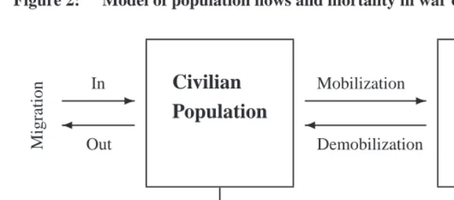
We propose a model based on the following population flows: As input stream for the civilian population we consider in-migration and demobilization, and the correspond-ing output stream includes out-migration, (civilian) deaths, and mobilization (see the flowchart in Figure 2). As to the combatant population, mobilization is the only input stream, whereas the output one includes (military) deaths and demobilization. Now that the streams are defined, our main goal is to determine all parts of input/output streams.
The equations can be formulated as follows. LetPc(t, y)be the number of persons alive at timet(on January 1st of yeart) in cohorty,Dc(t, y)is the number of civilian deaths in yeartand cohorty,M(t, y)is the net-migration between timetandt+ 1to cohorty. As to war time, the balance of change in the civilian population also includes the components described by mobilization: the number of conscripts Con(t, y), mobilized from cohortyin yeart, and the number of dischargeesDis(t, y), demobilized in yeart. Thus, for the civilian population we have the following equation3:
Pc(t+ 1, y) =Pc(t, y)−Dc(t, y)−Con(t, y) +Dis(t, y), t > y (1)
The equation for the military population can be written as
Pm(t+ 1, y) =Pm(t, y)−Dm(t, y) +Con(t, y)−Dis(t, y), t > y (2)
Figure 2: Model of population flows and mortality in war operations
Civilian
Population
Army
❄ Civilian Deaths
❄ Military Deaths ✲
Mobilization
✛
Demobilization ✲
In
✛ Out
Migration
wherePm andDm denote the military population (or members of the Armed Forces) and military deaths, respectively. When data for some of the components are available by aggregate age group only, if they are available at all, they can be reconstructed from these equations. Unfortunately, these equations would then have more than one solution. In other words, we need to choose one trajectory from a set of trajectories satisfying equa-tions (1) and (2). As a possible selection criterion we could use the maximum likelihood principle. However, then we would have to solve several problems. First, the large num-ber of unknown variables would have to be reduced. For example, given that the period of war is five years and all data except military deaths are known, we would need to apply a system of equations with 135 unknown variables4in order to reconstruct the age structure
of war related deaths. Second, we need to take into account that other demographic data (e.g., on migration) are hardly available or if they are, they are of questionable quality. Therefore, we are proposing the following assumptions that will solve the aforementioned problems.
3.2 Assumptions
a) The baseline probability of deaths is the same for both the non-civilian (members of the Armed Forces) and civilian populations5. An excess of mortality due to
war can be described by a gamma p.d.f. likely function with a maximum around age 18-20 (see examples of France (Vallin, 1973) or the Prudential life tables in Winter (1976)). Therefore, we use the sum of two probability density functions of the gamma distribution6 G1(x;b1, b2)andG2(x;b3, b4). The second function is introduced for a(n) (possible) additional peak at higher ages, i.e. 20-25 years. This peak may occur during Navy and Air Force operations resulting in a relative high number of casualties among the soldiers and officers more trained than others. Thus, the probability of deathqm(t, y)for military cohortyin yeartcan be defined via the civilian probability of death as follows:
qm(t, y) = qc(t, y) +b
0(t)∗(G1(t−y;b1(t), b2(t)) +
+G2(t−y;b3(t), b4(t))), (3)
whereb0(t)determines the relative levels of mortality by year, andb1(t)tob4(t) determine the shape of mortality distribution by age for every year.
b) Unknown migration should be minimized. It means that of all possible solutions of the balancing equation that satisfy the known data and conditions, the most likely solution is the one with minimal net migration. This allows us to define a number of conscripts and net migration even without knowing the strength of the Armed Forces.
c) Migration, mobilization, and demobilization are distributed uniformly within the elementary time intervals, i.e. the year or part of the year for mobilization/demo-bilization in the first/last year of war.
d) The process of mobilization stops with the end of the war. Soon after, for exam-ple before the first after-war census took place, all mobilized persons should be demobilized.
e) Initial populations at the start and the end points of the period considered in the model should agree with each other. Both of them should either include civilians
5Unfortunately, we are not able to consider any likely health selection effects as the Armed Forces tend to
recruit relatively healthy persons. Unhealthy persons, consequently unfit for military service, tends to be confined to the civilian population. This may have produced a slightly elevated mortality risk among the civilian population. Thus, taking the assumption of equal baseline probabilities of dying, we may have slightly over-estimated the mortality gap between the combat and civilian populations. Nevertheless, this effect will be negligible compared to mortality excess resulting from to war operations.
6The gamma probability density functionG(x;a, b)with parametersaandbis defined for each agexas
G(x;a, b) = 1 baΓ(a)xa−1e
x
only or civilians and combatants. This is the case for England and Wales: since populations counted by the last pre-war census and the first after-war census in-clude booth civilian and military parts.
3.3 Parameterized model
Taking into consideration the assumptions above, we modify the initial model (1)-(2). Let
tbeginbe the first calendar year of war,tenddenote the last year of war, andT represent the (first) year by which all additional troops have been demobilized. We assume that before yeartbegin, the total population is equivalent to the civilian population; in all other cases,tbegincan be defined as the first year of mobilization. For WWI,tbegin =1914,
tend=1918, andT =1921 (the year of the first post war census). Similarly, as to Second World War,tbegin=1939,tend=1945, andT =1951.
Suppose that the war began and ended on January 1st. Taking into account assumption (c), formula (1) for the “military” cohort can be written in the form of
Pc(t+ 1, y) = Pc(t, y)∗(1−qc(t, y)) +M(t, y), t < t
begin,
Pc(t+ 1, y) = Pc(t, y)∗(1−qc(t, y))−Con(t, y)∗
1 +12qc(t, y)
+
+Dis(t, y)∗
1−1
2q
c(t, y)
+M(t, y), tbegin≤t < tend,
Pc(t+ 1, y) = Pc(t, y)∗(1−qc(t, y)) +
+Dis(t, y)∗
1−12qc(t, y)
+M(t, y), tend≤t < T (4)
In other words, we can calculate the number of conscripts fortbegin≤t < tendas
Con(t, y) = Pc(t, y)∗(1−qc(t, y))−Pc(t+ 1, y)
1 +1
2qc(x, t)
+
+Dis(t, y)∗(1−12qc(t, y)) +M(t, y)
1 +1
2qc(x, t)
(5)
and the number of discharges fortend≤t < T as
Dis(t, y) = Pc(t+ 1, y)−Pc(t, y)∗(1−qc(t, y))−M(t, y)
1−1
2qc(x, t)
(6)
Pm(t+ 1, y) = Pm(t, y)∗(1−qm(t, y)) +Con(t, y)∗
1−12qm(t, y)
−
−Dist(t, y)∗
1 +12qm(t, y)
, (7)
fortbegin≤t < tend. Fortend≤t < T, the equation (7) is replaced by (8)
Pm(t+ 1, y) =Pm(t, y)∗(1−qm(t, y))−Dis(t, y)∗
1−1
2q
m(t, y)
(8)
withDis(t, y)from (6).
Above, we have assumed that data on migration are known. Unfortunately, the latter is a theoretical rather than a practical case. Data on net migration for England and Wales are available only for some years and merely by aggregate age groups. Furthermore, even these limited data seem to be hardly acceptable to our purposes due to their insufficient quality. During both war conditions, it was extremely difficult to follow inward and out-ward flows to and from the Armed Forces as many records of dischargees (e.g., due to injury) from the army were lost on the battlefields (Ellis, 1972). Some wounded soldiers possibly were included in the civilian population count without having entered them into official records of discharge from the army. These persons therefore have been counted twice, i.e., as “civilian” and as “soldier”.
Nevertheless, equation (5) can be adjusted according to data availability on different components. Net migration can be approximated by the parameterized function. In order to simplify the equation, we use the gamma probability density functionG3(x;k1, k2)for the further modeling of migration:
M(t, y) =k0(t)∗G3(t−y;k1(t), k2(t)), (9)
wherek0(t)determines the level of migration in yeart, andk1(t)andk2(t)determine the shape of the migration curve in each year.
Con(t, y) = Pc(t, y)∗(1−qc(t, y))−Pc(t+ 1, y) +M(t, y)
1 + 1
2qc(t, y)
, (10)
Pm(t+ 1, y) =Pm(t, y)∗(1−qm(t, y)) +Con(t, y)∗
1−1
2qm(t, y)
, (11)
Fortend ≤t < T, equation (11) is replaced by (8) withDis(t, y)from (6). Taking into account our assumption abouttbeginandT, we can define the first and last points in the model:
Pm(t
begin, y) =Pm(T, y) = 0,
Pc(t
begin, y) =P(tbegin, y),
Pc(T, y) =P(T, y). (12)
If we reject the assumption that the wars began and ended on January 1st, the number of conscripts is calculated as
Con(t, y) = Pc(t, y)∗(1−qc(t, y))−Pc(t+ 1, y) +M(t, y)
1 +1
2τtqc(x, t)
, (13)
whereτtis the war part of yeart. Correspondingly, the equation for demobilization is
Dis(t, y) =Pc(t+ 1, y)−Pc(t, y)∗(1−qc(t, y))−M(t, y)
1−1
2(1−τt)∗qc(x, t)
, (14)
3.4 The minimization functional
λ1
tbegin<t<tend
Dm(t)−1
y
Dm(t, y)−Da(t)
2
+
+ λ2
tbegin<t<tend
Pm(t)−1
y
Pm(t, y)−Pm(t)
2
+
+ λ3
tbegin<t<T
y
Pc(t, y)2
−1
y
M(t, y)2+ (15)
+ λ4
tend<t<T
Pa(t
begin+ 1)−2
y
(t−tend)Pm(t, y)2→ min
b0,...,bn,k0,...,km
.
Here,Da(t)denotes the total number of military deaths in yeart,Pa(t)is the strength of the army in yeart. The terms define the discrepancy between the estimated number of deaths and the total number of deaths known, the discrepancy in population estimates, mi-gration, and army strength after the war, respectively. Coefficientsλ1, . . . , λ4determine the relative weight of terms and depend on the quality and importance of the different parts of available data. Their values determine the relative importance of decrease in the respective term. For example, an increase inλ1 promotes a decrease in the difference between the estimated number of deaths and the known total number of deaths. It is clear that the differences between official and simulated data have a greater importance than the level of migration and army strength after the war. Moreover, as death statistics usually are more reliable, we should takeλ1λi, i= 2,3,4. We have tested different ratios of
λi, i= 1, . . . ,4and selected the set of coefficients which produces the closest and most
reliable result compared to the outcomes of other studies. As to the minimization func-tional (15) for WWI, we apply the following coefficients:λ1= 10, λ2= 5, λ3 = 1, and
λ4= 0.1. Figure 3 shows the sensitivity of the fit of combatant deaths and the strength of
the army to changes in lambdas. Four panels of Figure 3 correspond to one-dimensional variations in eachλi, i= 1, . . . ,4by holding the values of the other lambdas constant. As one can see, for each lambda there is an interval of acceptable values with minimal differ-ences between estimations and official data. Within these intervals, the resulting fits are almost independent of the exact values of the lambdas. It means that the proposed model is stable in respect to parametersλi, i= 1, . . . ,4and that small changes inλihave only a negligible impact on mortality estimates. More precise and reliable data are available for WWII, and this invites us to employ another value of coefficientλ2. We takeλ2 = 8to increase the weight of the population estimation in the functional to be minimized.
year age groups, army strength for years of warPm(t), and distributions of total mili-tary deaths by years of warDm(t). We have nine parameters for each year of war (see equations (3), (9)-(11)) and three parameters for each postwar year (see (8) and (9)). To choose these variables, we need to minimize the functional (15). As output, we get the combatant population and military deaths by one-year age group for each calendar year before the first after-war census.
Figure 3: Dependence of the fit of total combatant deaths (1914-1918) and army strength (1914-1917) on changes ofλi, i= 1, . . . ,4
4. Results
4.1 The First World War
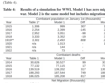
We apply the following assumptions related to net migration during the First World War. Net migration is zero during the war years. Model 1 includes post-war net migration only. As an alternative we consider a model with migration during the war (Model 2). Both models produce reasonable results, which are concordant with other data sources (Table 4).
Table 4: Results of a simulation for WWI. Model 1 has zero migration during the war. Model 2 is the same model but includes migration in times of war
Combatant population on January 1st (thousands)
Year Table 1* Model 1 Diff Model 2 Diff
1915 1,306 999 307 1,306 0
1916 2,254 2,399 -145 2,269 -15
1917 2,952 3,051 -98 2,952 0
1918 3,333 3,352 -19 3,333 0
1919** 3,301 2,493 808 2,552 749
1920 n/a 1,013 - 1,076
-1921 n/a 144 - 185
-1922 n/a 73 - 81
-Combatant deaths
Year Table 1 Model 1 Diff Model 2 Diff
1914 30,626 30,527 99 30,591 35
1915 77,132 77,115 17 77,107 25
1916 139,519 139,202 317 139,591 -72
1917 188,293 187,544 749 188,322 -29
1918 186,025 185,208 817 186,041 -16
Net Migration (thousands)
Year Official Model 1 Diff Model 2 Diff
1914 n/a 0 - 306
-1915 n/a 0 - -442
-1916 n/a 0 - 27
-1917 n/a 0 - 77
-1918 n/a 0 - 76
-1919 n/a 1.2 - 1.3
-1920 n/a 1.2 - 1.4
-1921 n/a 1.4 - 1.4
-* Calculated as a weighted average from Table 1
** Official data given on 01.11.1918
the rules of migration minimization (see assumption (b) in the third section), the model with zero migration during the war years has been selected to reconstruct the mortality surface for England and Wales for the period around the First World War. For the further verification of Model 1, the age patterns of deaths and mortality have been compared to the corresponding estimates published by Winter (1976, 2003) (Figure 4). Although the estimated age-specific mortality curves look more smoothed, they show almost identical increases in mortality at ages 19-24 compared to the data on Prudential policy holders re-published by Winter (2003).
The reconstruction of the mortality surface for the total population of England and Wales enabled us to produce new continuous series of life tables for the years around the First World War. As expected, the effect of war loss is great. Compared to civilian males, the decrease in life expectancy at birth among the total of males was more rapid, showing a decline by 18 years between 1913 and 1918. Among the civilian males, the corresponding drop was about 10 years, suggesting that military casualties may have been included in part in the official statistics. The flu epidemic in 1918 is an additional factor that explains the peak in civilian deaths. As for females, the adjustments made have a negligible effect on the mortality trends for the period around the First World War.
Our results provide some insights into the age patterns of total population losses dur-ing the First World War. Figure 5 shows that the most strikdur-ing excess male mortality in the total population has affected the ages 18-24, with the maximum peak being age at 23 in 1918. Between 1913 and 1918, the latter age shows a 15-16 fold increase in the proba-bility of dying. At the same time, and according to the unadjusted official figures for the civilian population, males belonging to the same age interval experience only a three to four-fold jump in mortality risk. The inclusion of a combatant part of the population has a significant impact on the life expectancy indicators for the 1885-1899 cohorts (Figure 5). The maximum difference between adjusted and unadjusted series (based on the civilian population only) is almost four years in the 1896 cohort, i.e., for men aged 18 in 1914.
Figure 5: Life expectancy at birth for the 1870-1910 cohorts, calculated from civilian and adjusted (total) data
4.2 The Second World War
Data on the military population during WW II are available at a much more detailed level (see Section 2 for more details). Thus, functional (15) requires only slight modifications to fit the additional data. The adjustment concerns the second term, which defines population size. As the data on the combatant population are available by five-year age groups and for each year of the war, we modify the model as follows:
λ1
tbegin<t<tend
Dm(t)−1
y
Dm(t, y)−Da(t)
2
+
+ λ2
tbegin<t<tend
Pm(t)−1
yi<y≤yi+1
Pm(t, y)−Pm(t, y
i:yi+1) 2 +
+ λ3
tbegin<t<T
y
Pc(t, y)2
−1
y
M(t, y)2+ (16)
+ λ4
tend<t<T
Pa(t
begin+ 1)−2
y
(t−tend)Pm(t, y)2→ min
b0,...,bn,k0,...,km
,
wherePm(t, y
i:yi+1)is the population size for age group[t−yi+1, t−yi]int. Similarly to WWI, we used as initial time point January 1st, 1939; the last time point was the date of the first postwar census (1951).
Overall, our results are very close to those yielded by the available official data on the total and military populations. For example, the estimated military deaths show no difference to the official statistics except for a negligible gap of around 0.15% (27 deaths) for 1941. The estimated and official population counts are also almost identical, with a maximum difference of less than 0.1% over all age groups and years.
specific conditions of war. The number of civilian deaths owing to air strikes of the enemy was very close to the number of military deaths (in action) at the beginning of the war.
Figure 6: Probability of death at age 25 for the civilian and total population, England and Wales, males (left); life expectancy at age 0 for civilian and total population, England and Wales, males (right)
The reconstructed age-specific mortality patterns demonstrate that the growth of male mortality among the total population of England and Wales mostly concentrated on the ages 18-25 (as with the First World War), showing a five to seven-fold increases in mor-tality risk between 1938 and 1945 (Figure 7). The maximum level of mormor-tality is held in 1945 by males aged 21, an age two years younger compared to 1918.
The inclusion of the combatant population figures has a modest impact on the cohort mortality indicators. For example, the average life expectancy between ages 0 and 70 for the 1919 cohorts of the civilian and “total” population shows a maximum difference of 1.15 years (see Figure 8). Figures 6 and 8 confirm that the effect of WWII on mortality among the total population is less important than that of WWI. Unfortunately, it was not possible to validate our results on age-specific mortality patterns (as we did for the First World War).
5. Conclusion
We reconstructed a continuous series for war-time England and Wales, which includes estimates of the non-civilian population and deaths in war operations. We used the same model for both world wars. The adjusted data on England and Wales show significant effects of excess mortality among the military population on life expectancy trends in the total population during both wars.
compo-Figure 7: Probability of death for the “total” population by age groups, 1938-1945, England and Wales, males. Results of simulation
nents of the population movement. We showed that this modeling approach combined with a set of assumptions can be successfully applied to the estimation of mortality sur-faces.
The modeling procedures applied in our study can be easily modified to become ap-plicable under the conditions where even less data are available (the data for the censuses before and after the war being an exception, as they are complete). However, the relia-bility of the resulting estimates fully depends on the level of availarelia-bility and quality of the data used for the modeling. We hope that the proposed method of mortality pattern reconstruction can be successfully applied to data on other countries that suffer from the exclusion of the military population from the statistics during the First and Second World War.
6. Acknowledgements
References
Brooke, E. (1972). The Emergency Medical Services. Medical Statistics. Casualties
and Medical Statistics. History of the Second World War (United Kingdom Medical Series), Ed.: W.F. Mellor, HMSO, London, 635-825.
Burn, J. (1918). Industrial mortality 1915-1917. Journal of the Institute of Actuaries, 51, pp. 67-71.
Central Statistical Office (CSO). (1951, reprinted in 1995). Fighting with Figures. A Statistical Digest of the Second World War, Central Statistical Office, HMSO,
London, 298 p.
Dudley, S. (1942). Discussion on Professor Greenwood’s paper. Journal of the Royal
Statistical Society, 105(1), pp. 12-13.
Ellis, F. (1972). The Royal Naval Medical Services. Medical Statistics. Casualties
and Medical Statistics. History of the Second World War (United Kingdom Medical Series), Ed.: W.F. Mellor, HMSO, London, pp. 1-90.
HMSO. (1972). Casualties and Medical Statistics. History of the Second World War (United Kingdom Medical Series), Ed.: W.F. Mellor, HMSO, London, 893 p.
Mayne, H. (1972). The Army Medical Services. Medical Statistics. Casualties and
Medical Statistics. History of the Second World War (United Kingdom Medical Series), Ed.: W.F. Mellor, HMSO, London, pp. 91-454.
Mitchell, T.J., Smith, G.M. (1931, reprinted in 1997). Casualties and medical statistics
of the Great War, Army Medical Services, His Majesty’s Stationery Office, London,
402 p.
The Army Council. (1921). General Annual Report of the British Army 1913-1919 (prepared by command of the Army Council). Parliamentary Paper 1921, XX, Cmd.1193.
The Army Service Forces, War Department. (1956). The Emergency Medical Ser-vices. Medical Statistics. Statistical Review. World War II, Downloaded from
www.maxwell.af.mil/au/afhra/wwwroot/aafsd/aafsd list of tables.html.
The War Office. (1922). The Emergency Medical Services. Medical Statistics. Statistics
of Military Effort of the British Empire during the Great War, 1914-1920, HMSO,
London, 635-825.
Urlanis, B. (1971). Wars and Population, Progress Publishers, Moscow, 320 p.
Vallin, J. (1973). La mortalite par generation in France, depuis 1899., Paris: INED &
Presses Universitaries de France, 484 p.
Welch, S. (1972). The Royal Air Force Medical Services. Medical Statistics. Casualties
and Medical Statistics. History of the Second World War (United Kingdom Medical Series), Ed.: W.F. Mellor, HMSO, London, pp. 455-633.
Winter, J. (1976). Some aspects of the demographic consequences of the First World War in Britain. Population Studies, 30(3), pp. 539-552.
Winter, J. (1977). Britain’s “lost generation” of the First World War. Population Studies,
31(3), pp. 449-466.