An efficient improvement of the Newton method for solving
non-convex optimization problems
Tayebeh Dehghan Niri∗
Department of Mathematics, Yazd University, P. O. Box 89195-74, Yazd, Iran.
E-mail: [email protected], T. [email protected]
Mohammad Mehdi Hosseini
Department of Mathematics, Yazd University, P. O. Box 89195-74, Yazd, Iran.
E-mail: hosse−[email protected] Mohammad Heydari
Department of Mathematics, Yazd University, P. O. Box 89195-74, Yazd, Iran.
E-mail: [email protected]
Abstract Newton method is one of the most famous numerical methods among the line search methods to minimize functions. It is well known that the search direction and step length play important roles in this class of methods to solve optimization problems. In this investigation, a new modification of the Newton method to solve uncon-strained optimization problems is presented. The significant merit of the proposed method is that the step length αk at each iteration is equal to 1. Additionally, the convergence analysis for this iterative algorithm is established under suitable conditions. Some illustrative examples are provided to show the validity and ap-plicability of the presented method and a comparison is made with several other existing methods.
Keywords. Unconstrained optimization, Newton method, Line search methods, Global convergence. 2010 Mathematics Subject Classification. 65K05, 90C26, 90C30, 49M15.
1. Introduction
Letf :Rn →Rbe twice continuously differentiable and smooth function. Consider
the minimization problem
min
x∈Rnf(x), (1.1)
and assume that the solution set of (1.1) is nonempty. Among the optimization methods, classical Newton method is well known for its fast convergence property. However, the Newton step size may not be a descent direction of the objective func-tion or even not well defined when the Hessian is not a positive definite matrix.
Received: 26 March 2017 ; Accepted: 23 October 2018.
∗Corresponding author.
There are many improvements of the Newton method for unconstrained optimization to achieve convergence. Zhou et al. [24] presented a new method for monotone equa-tions, and showed its superlinear convergence under a local error-bound assumption that is weaker than the standard nonsingularity condition. Li et al. [11] obtained two regularized Newton methods for convex minimization problems in which the Hessian at solutions may be singular and showed that iff is twice continuously differentiable, then the methods possess local quadratic convergence under a local error bound con-dition without requiring isolated nonsingular solutions. Ueda and Yamashita [21] ap-plied a regularized algorithm for nonconvex minimization problems. They presented a global complexity bound and analyzed the super linear convergence of their method. Polyak [16] proposed the regularized Newton method for unconstrained convex opti-mization. For any convex function, with a bounded optimal set, the RNM (regularized Newton method) generates a sequence converging to the optimal set from any starting point. Shen et al. [19] proposed a regularized Newton method to solve unconstrained nonconvex minimization problems without assuming the non-singularity of solutions. They also proved its global and fast local convergences under suitable conditions.
In this paper, we propose a new algorithm to solve unconstrained optimization problems. The organization of the paper is as follows: In section 2, we introduce a new regularized method to solve minimization problems. Section 3 presents the global convergence analysis of our algorithm. Some preliminary numerical results are reported in section 4 and some concluding remarks are presented in the final section.
2. Regularized Newton method We consider the unconstrained minimization problem,
min
x∈Rnf(x), (2.1)
wheref :Rn−→Ris twice continuously differentiable. We suppose that, for a given
x0∈Rn, the level set
L0={x∈Rn|f(x)≤f(x0)}, (2.2)
is compact. Gradient ∇f(x) and Hessian ∇2f(x) are denoted by g(x) and H(x),
respectively. In general, numerical methods, based on line search to solve the problem (2.1) have the following iterative formula
xk+1=xk+αkpk, (2.3)
wherexk, αkandpkare current iterative point, a positive step size and a search
direc-tion, respectively. The success of linear search methods depends on the appropriate selections of step length αk and direction pk. Most line search methods require pk
to be a descent direction, since this property guarantees that the functionf can be decreased along this direction.
For example, the steepest descent direction is represented by
pk =−gk, (2.4)
and Newton-type direction uses
Generally, the search direction can be defined as
pk=−Bk−1∇fk, (2.6)
whereBk is a symmetric and nonsingular matrix. IfBk is not positive definite, or is
close to being singular, then one can modify this matrix before or during the solution process. A general description of this modification is presented as follows [15].
Algorithm 1. (Line Search Newton with Modification ): For given initial pointx0and parameters α >0, β >0;
while∇f(xk)̸= 0
Factorize the matrixBk=∇2f(xk) +Ek,
whereEk = 0 if∇2f(xk) is sufficiently positive definite;
otherwise,Ek is chosen to ensure thatBk is sufficiently positive definite;
SolveBkpk =−∇f(xk);
Setxk+1=xk+αkpk ,
whereαk satisfies the Wolfe, Goldstein, or Armijo backtracking conditions.
end while.
The choice of Hessian modificationEk is crucial to the effectiveness of the method.
2.1. The regularized Newton method. Newton method is one of the most popular methods in optimization and to find a simple rootδof a nonlinear equationf(x), i.e., f(δ) = 0 in casef′(δ)̸= 0, by using
xk+1 =xk−
f(xk)
f′(xk)
, k= 0,1, . . . , (2.7)
that converges quadratically in some neighborhoods ofδ[20,3]. The modified Newton method for multiple rootδof multiplicitym, i.e.,f(j)(δ) = 0, j= 0,1, . . . , m−1 and
f(m)(δ)̸= 0, is quadratically convergent and it is written as xk+1=xk−m
f(xk)
f′(xk)
, k= 0,1, . . . , (2.8)
which requires the knowledge of the multiplicitym. If the multiplicitymis unknown, the standard Newton method has a linear convergence with a rate of (m−1)/m [4]. Traub in [20] used a transformation µ(x) = ff′((xx)) instead of f(x) to compute a
multiple root off(x) = 0. Then the problem of finding a multiple root is reduced to the problem of finding a simple root of the transformed equationµ(x), and thus any iterative method can be used to maintain its original convergence order. Applying the standard Newton method (2.7) toµ(x) = 0, we can obtain
xk+1=xk−
f(xk)f′(xk)
f′(xk)2−f(xk)f′′(xk)
, k= 0,1, . . . . (2.9) This method can be extended ton-variable functions as
Xk+1=Xk−
(
∇f(Xk)∇f(Xk) T−
f(Xk)∇2f(Xk)
)−1
fork= 0,1, . . . .
In this section, we introduce a new search direction for the Newton method. The presented method is obtained by investigating the following parametric family of the iterative method
Xk+1=Xk−
(
β∇f(Xk).∇f(Xk) T−
f(Xk)∇
2 f(Xk)
)−1
θf(Xk)∇f(Xk), (2.11)
whereθ, β∈R− {0} are parameters to be determined andk= 0,1, . . . .
Whenθ=β= 2, (2.11) reduces to the Halley method [12,18], which is defined by Xk+1=Xk−
(
2∇f(Xk).∇f(Xk)T−f(Xk)∇2f(Xk)
)−1
2f(Xk)∇f(Xk), (2.12)
fork= 0,1, . . . .
Remark 2.1. If β = 0 and θ =−1, the proposed method reduces to the classical Newton method,
Xk+1=Xk−
(
∇2f(X k)
)−1
∇f(Xk), k= 0,1, . . . .
Now, we present a general algorithm to solve unconstrained optimization problems by using (2.11).
Algorithm 2. (Regularized Newton method): Step 1. Given initial pointx0,τ >0,θ,β andϵ. Step 2. If∥fkgk∥= 0 stop.
Step 3. IfBk= (βgkgTk −fkHk) is a nonsingular matrix then
Solve (βgkgTk −fkHk)pk=−θfkgk;
else
Solve (βgkgTk −fkHk+τ I)pk=−θfkgk;
Step 4. xk+1=xk+pk.
Setk:=k+ 1 and go to Step 2.
We remind that Bk = (βgkgkT −fkHk) is a symmetric matrix. This algorithm is
a simple regularized Newton method.
3. Global convergence
In this section, we study the global convergence of Algorithm 2. We first give the following assumptions.
Assumption 3.1.
(A1): The mappingf is twice continuously differentiable, below bounded and the level set
is bounded.
(A2): g(x)∈Rn×1 andH(x)∈ Rn×n are both Lipschitz continuous that is, there exists a constantL >0 such that
∥g(x)−g(y)∥ ≤L∥x−y∥, x, y∈Rn, (3.2) and
∥H(x)−H(y)∥ ≤L∥x−y∥, x, y∈Rn. (3.3)
(A3): β∈R− {0} and 2β(∇fkT(fk∇2fk)−1∇fk)≤1.
Theorem 3.2. SupposeAis a nonsingularN×N matrix,U isN×M,V isM×N,
thenA+U V is nonsingular if and only ifI+V A−1U is a nonsingularM×M matrix.
If this is the case, then
(A+U V)−1=A−1−A−1U(I+V A−1U)−1V A−1.
This is the Sherman-Morrison-Woodbury formula [10, 9, 22]. See [10] for further generalizations.
Proposition 3.3. [10]Let B be a nonsingular n×nmatrix and letu, v∈Rn. Then
B+uvT is invertible if and only if1 +vTB−1u̸= 0. In this case,
(B+uvT)−1=(I− B−1uvT
1+vTB−1u
) B−1.
Lemma 3.4. Suppose that Assumption3.1 (A1)and(A3)hold. Then
(I) ∇f
T k(
−fk β ∇
2f
k)−1∇fk
1+∇fT k(
−fk
β ∇2fk)−1∇fk ≤1,
(II) (−fk
β ∇
2f
k+∇fk∇fkT)− 1=−β
fk(∇
2f
k)−1(I−
∇fk∇fkT( −fk
β ∇
2f
k)−1
1+∇fT k(
−fk
β ∇2fk)−1∇fk ).
Proof. From Assumption3.1 (A3), we have
β(∇fkT(−fk∇2fk)−1∇fk)≥ −
1 2 =⇒ ∇f
T k(
−fk
β ∇ 2
fk)−1∇fk≥ −
1
2, (3.4)
and hence
∇f
T k(−
fk
β ∇
2f
k)−1∇fk
1 +∇fT k(−
fk
β ∇2fk)−1∇fk
≤1.
According to Theorem3.2and Proposition3.3, we set B= −fk
β ∇
2f
k, u=v =∇fk.
From (3.4) we obtain
1 +vTB−1u= 1 +∇fkT(−fk β ∇
2f
k)−1∇fk ≥
1 2. Therefore, the matrixB+uvT is invertible and we can get
(B+uvT)−1= (−fk
β ∇
2f
k+∇fk∇fkT)−1
= (−fk
β ∇
2
fk)−1−(−βfk∇2fk)−1∇fk(1 +∇fkT(− fk β ∇
2
fk)−1∇fk)−1∇fkT(− fk β ∇
2 fk)−1
=−fβ
k(∇ 2
fk)−1(I−
∇fk∇fkT( −fk
β ∇2fk)−1 1+∇fT
k( −fk
β ∇2fk)−1∇fk
).
Theorem 3.5. Suppose that the sequence{xk}generated by Algorithm 2 is bounded. Then we have
lim k→∞∥
fkgk∥= 0.
Proof. First, we prove thatpk is bounded. Suppose thatγ=L∥(∇2f(x∗))−1∥. From
the definitions ofpk in Algorithm 2, we have ∥pk∥ ≤ |θ|.∥(∇2f(xk))−1∥.∥∇f(xk)∥ ≤
2|θ|γ
L ∥∇f(xk)∥, suppose that{xk} ⊆Λ andC= supx∈Λ{∥∇fk∥}<+∞, therefore
∥pk∥ ≤
2|θ|γ L C,
which proves thatpk is bounded for allk. By Taylor Theorem, we have
f(xk+pk) =f(xk) +∇fkTpk+
1 2p
T k∇
2
f(xk+tpk)pk
=f(xk) +∇fkTpk+O(∥pk∥2),
therefore by the boundedness ofpk
f(xk+pk)−f(xk)−σ∇fkTpk = (1−σ)∇fkTpk+O(∥pk∥2)
=−(1−σ)∇fkTB− 1
k fk∇fk+O(∥pk∥2).
If∇fT kB−
1
k fk∇fk>0,then
f(xk+pk)−f(xk)−σ∇fkTpk≤0,
therefore
f(xk+pk)≤f(xk) +σ∇fkTpk. (3.5)
Hence, the sequence {f(xk)} is decreasing. Sincef(x) is bounded below, it follows
that
lim k→∞
fk =f ,
wheref is a constant. Now we prove that lim
k→∞∇
fkTBk−1fk∇fk = 0. (3.6)
With assuming∇fT kB−
1
k fk∇fk >0 there exists a scalarϵ >0 and an infinite index
set Γ such that∇fT kB−
1
k fk∇fk> ϵfor allk∈Γ. According to (3.5), we obtain
f(xk+pk)−f(xk)≤σ∇fkTpk. (3.7)
Then
f−f(x0) = ∞
∑
k=0
(f(xk+1)−f(xk))≤
∑
k∈Γ
(f(xk+1)−f(xk))≤
∑
k∈Γ
σ∇fkTpk
=−∑
k∈Γ
This implies that∇fkTBk−1fk∇fk → 0 ask→ ∞ and k ∈Γ,which contradicts the
fact ∇fkTBk−1fk∇fk > ϵ, k∈ Γ. Hence, the whole sequence {∇fkTB− 1
k fk∇fk} tends
to zero.
Assumption3.1(A2)and the boundedness of{xk} show that
λmax
( Bk−1fk
)
≤λ, (3.8)
for allk,whereλis a positive constant. Therefore due to matrices property,λmin(Bk−1fk)≥
b
λfor some constantbλ >0.Hence,∇fT kB−
1
k fk∇fk ≥bλfk∥∇f(xk)∥
2. Then from (3.6),
∥fkgk∥ −→0 ask→ ∞.
4. Numerical results
In this section, we report some results on the following numerical experiments for the proposed algorithm. In addition, we have compared the effectiveness of the proposed method with the Improved Cholesky factorization, ([15], Chapter 6, Page 148) regularized Newton (RN) [7] and Halley method [12]. In Algorithm 2, we have used τ = 10−6 and in Improved Cholesky factorization (LDLT), we have assumed
c1 = 10−4, α0= 1, ρ= 12, δ =√eps and ϵ= 10−5.Furthermore, Improved Cholesky
factorization uses the Armijo step size rule. Nf andNg represent the number of the
objective function and its gradient evaluations, respectively. All these algorithms are implemented in Matlab 12.0. The test functions are commonly used for unconstrained test problems with standard starting points and summary of them are given in Table 1 [1,2,13].
Table 1. Test problems [1,2,13].
No. Name No. Name
1 Powell Singular 16 NONDQUAR
2 Extended Beale 17 ARWHEAD
3 HIMMELH 18 Broyden Tridiagonal
4 SINE 19 Extended DENSCHNB
5 FLETCHCR 20 Extended Trigonometric
6 LIARWHD 21 Extended Himmelblau
7 DQDRTIC 22 Extended Block Diagonal BD1
8 NONSCOMP 23 Full Hessian FH2
9 NONDIA 24 EG2
10 wood 25 EG3
11 Brown badly scaled 26 ENGVAL8
12 Griewank 27 Generalized Quartic
13 Extended Powell 28 Broyden Pentadagonal 14 Diagonal Double Bounded Arrow Up 29 Freudenstein and Roth
15 Diagonal full borded 30 INDEF
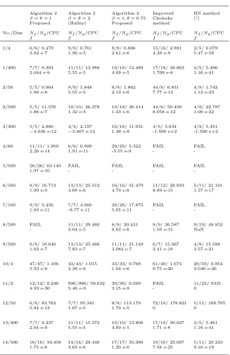
Table 2. Numerical results.
Algorithm 2 Algorithm 2 Algorithm 2 Improved RN method
β=θ= 1 β=θ= 2 β= 1, θ= 0.75 Cholesky [7] Proposed (Halley) Proposed method
No./Dim Nf/Ng/CPU Nf/Ng/CPU Nf/Ng/CPU Nf/Ng/CPU Nf/Ng/CPU
f f f f f
1/4 6/6/ 0.479 9/9/ 0.761 8/8/ 0.666 15/16/ 2.881 2/5/ 0.079 3.82 e-7 1.96 e-5 2.61 e-6 4.38 e-9 5.47 e-58
1/400 7/7/ 8.303 11/11/ 13.988 10/10/ 12.489 17/18/ 29.863 2/5/ 5.496 2.044 e-9 5.55 e-5 4.09 e-5 1.709 e-8 1.16 e-41
2/50 5/5/ 0.964 9/9/ 1.848 9/9/ 1.862 44/9/ 6.851 4/9/ 1.742 1.90 e-8 5.55 e-5 2.19 e-6 7.77 e-13 1.12 e-23
2/500 5/5/ 11.576 10/10/ 26.378 10/10/ 26.414 44/9/ 50.450 4/9/ 22.787 1.86 e-7 1.32 e-5 1.43 e-6 8.058 e-12 1.09 e-22
3/300 5/5/ 2.880 4/4/ 2.197 16/16/ 11.031 4/5/ 3.634 4/9/ 5.451 −4.036 e-12 −3.467 e-12 1.48 e-8 -1.500 e+2 -1.500 e+2
4/60 11/11/ 1.959 6/6/ 0.999 29/29/ 5.322 FAIL FAIL 2.26 e-14 1.91 e-11 -3.55 e-9 -
-5/500 26/26/ 63.140 FAIL FAIL FAIL FAIL
1.97 e-10 - - -
-6/500 9/9/ 16.713 13/13/ 25.312 16/16/ 31.479 11/12/ 28.933 5/11/ 21.101 1.09 e-9 4.68 e-6 4.79 e-6 8.89 e-15 1.57 e-17
7/100 9/9/ 5.456 7/7/ 4.060 28/28/ 17.875 FAIL FAIL
1.93 e-11 -8.77 e-11 5.05 e-11 -
-8/500 FAIL 11/11/ 29.460 8/8/ 20.431 8/9/ 26.587 9/19/ 48.852
- 3.04 e-5 9.82 e-6 1.50 e-15 NaN
9/500 6/6/ 10.646 13/13/ 25.466 11/11/ 21.149 6/7/ 15.367 4/9/ 15.588 1.02 e-7 7.83 e-7 3.082 e-7 2.41 e-19 3.57 e-21
10/4 47/47/ 1.106 43/43/ 1.015 33/33/ 0.768 61/40/ 1.674 29/59/ 0.954 5.93 e-9 2.38 e-6 1.04 e-6 8.75 e-20 3.046 e-26
11/2 12/12/ 0.246 996/996/ 59.632 30/30/ 0.509 FAIL 11/23/ 0331
4.93 e-30 5.46 e-9 3.15 e-9 - 0
12/50 6/6/ 83.762 7/7/ 95.341 8/8/ 113.179 72/10/ 178.821 5/11/ 160.765
5.94 e-13 1.67 e-5 1.79 e-5 0 0
13/400 7/7/ 9.237 11/11/ 15.372 10/10/ 13.806 17/18/ 30.827 2/5/ 5.461 2.04 e-9 5.55 e-5 4.09 e-5 1.71 e-8 1.16 e-41
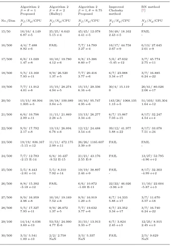
Table 3. Numerical results.
Algorithm 2 Algorithm 2 Algorithm 2 Improved RN method
β=θ= 1 β=θ= 2 β= 1, θ= 0.75 Cholesky [7] Proposed (Halley) Proposed method
No./Dim Nf/Ng/CPU Nf/Ng/CPU Nf/Ng/CPU Nf/Ng/CPU Nf/Ng/CPU
f f f f f
15/50 16/16/ 4.149 25/25/ 6.643 45/45/ 12.078 59/48/ 18.162 FAIL
6.87 e-5 5.15 e-4 4.41 e-5 2.43 e-5
-16/500 4/4/ 7.488 FAIL 7/7/ 14.789 16/17/ 44.758 6/13/ 27.645
8.92 e-6 - 3.27 e-4 2.67 e-9 2.61 e-9
17/500 6/6/ 11.029 10/10/ 19.780 8/8/ 15.386 5/6/ 47.632 3/7/ 45.774 1.47 e-8 4.12 e-6 8.60 e-7 -5.45 e-12 2.75 e-11
18/500 5/5/ 13.160 9/9/ 26.520 7/7/ 20.416 6/7/ 23.988 3/7/ 16.885 7.93 e-11 1.37 e-5 3.77 e-6 3.34 e-17 6.24 e-22
19/500 7/7/ 11.912 15/15/ 28.274 15/15/ 29.336 30/4/ 15.119 20/41/ 80.026
4.01 e-8 4.94 e-5 6.16 e-6 0 2.06 e-17
20/50 15/15/ 89.994 18/18/ 109.089 16/16/ 95.747 143/26/ 1068.135 51/103/ 535.304 1.005 e-5 3.84 e-5 4.95 e-6 1.13 e-5 1.64 e-12
21/500 6/6/ 10.798 11/11/ 21.869 13/13/ 26.277 6/7/ 15.867 8/17/ 32.247 2.09 e-11 2.26 e-5 3.34 e-6 7.03 e-15 4.54 e+4
22/500 9/9/ 17.792 13/13/ 26.894 12/12/ 24.488 39/12/ 41.977 8/17/ 33.078 2.17 e-8 6.76 e-6 3.54 e-6 5.88 e-22 7.51 e-24
23/500 19/19/ 836.167 11/11/ 472.175 26/26/ 1165.607 FAIL FAIL
-5.15 e-12 2.99 e-11 3.39 e-9 -
-24/500 7/7/ 12.783 6/6/ 10.427 21/21/ 43.176 FAIL 13/27/ 52.795 -2.15 E-14 -9.52 E-15 2.55 E-9 - -4.96 e+2
25/500 5/5/ 8.443 5/5/ 8.310 19/19/ 38.897 FAIL 8/17/ 32.303
-2.81 e-14 7.92 e-14 2.46 e-9 - -4.99 e+2
26/500 8/8/ 15.392 FAIL 6/6/ 10.872 22/22/ 46.026 11/10/ 22.604 -3.18 e-12 - -1.00 E-11 -3.96 e-9 -5.87 e+3
27/500 9/9/ 16.959 10/10/ 19.169 9/9/ 16.919 6/7/ 14.333 3/7/ 11.670 2.98 e-8 7.52 e-6 1.29 e-5 5.88 e-17 3.57 e-18
28/500 5/5/ 17.327 9/9/ 26.072 7/7/ 19.632 6/7/ 23.352 3/7/ 16.740 7.93 e-11 1.37 e-5 3.77 e-6 3.34 e-17 6.24 e-22
29/100 14/14/ 6.036 53/53/ 24.900 31/31/ 13.913 6/7/ 3.824 12/25/ 8.915 3.69 e-13 4.77 E-6 3.33 e-7 2.45 e+3 2.45 e+3
30/500 3/3/ 5.541 2/2/ 2.758 3/3/ 5.337 FAIL 2/5/ 9.629
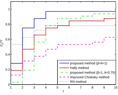
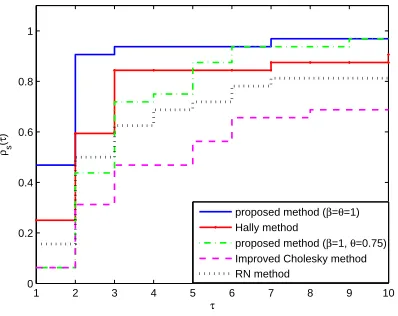
Recently, to compare iterative algorithms, Dolan and More’ [8], proposed a new tech-nique comparing the considered algorithms with statistical process by demonstrating performance profiles. In this process, it is known that the plot of the performance profile reveals all of the major performance characteristics, which is a common tool to graphically compare effectiveness as well as robustness of the algorithms. In this technique, one can choose a performance index as a measure of comparison among considered algorithms and can illustrate the results with performance profile. We use the three measuresNf, Ng and CP U time to compare these algorithms. Hence, we
use these three indices for all of the presented algorithms separately. Figures 1, 2 and 3 show the performance of the mentioned algorithms relative to these metrics, respectively.
Figure 1. Performance profile for the number of the objective func-tion evaluafunc-tions.
1 2 3 4 5 6 7 8 9 10
0 0.2 0.4 0.6 0.8 1
τ
ρs
(
τ
)
proposed method (β=θ=1) Hally method
proposed method (β=1, θ=0.75) Improved Cholesky method RN method
4.1. Systems of nonlinear equations. In this part, we solve systems of nonlinear equations by using the proposed algorithm. Consider the following nonlinear system of equations
F(x) = 0, (4.1)
whereF(x) = (f1(x), f2(x), . . . , fn(x)) andx∈Rn. This system can be extended as
f1(x1, x2, . . . , xn) = 0,
f2(x1, x2, . . . , xn) = 0,
.. .
fn(x1, x2, . . . , xn) = 0.
For solving (4.1) by proposed algorithm, we suppose thatf(x) =
n
∑
i=1
fi2(x). Here, we
Figure 2. Performance profile for the number of gradient evaluations.
1 2 3 4 5 6 7 8 9 10
0 0.2 0.4 0.6 0.8 1
τ
ρs
(
τ
)
proposed method (β=θ=1) Hally method
proposed method (β=1, θ=0.75) Improved Cholesky method RN method
Figure 3. Performance profile for CPU time.
1 2 3 4 5 6 7 8 9 10
0 0.2 0.4 0.6 0.8 1
τ
ρs
(
τ
)
proposed method (β=θ=1) Hally method
proposed method (β=1, θ=0.75) Improved Cholesky method RN method
the stopping criterion is given by∥f(xk)∥<10−8.
The numerical results of Examples 1,2 and 3 are given in Tables 3, 4 and 5, respec-tively.
Example 1. [14]:
F(X) = {
x31−3x1x22−1 = 0,
3x2x21−x32+ 1 = 0,
X1∗= (−0.290514555507,1.0842150814913),
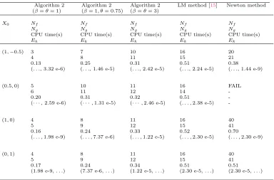
Table 4. Numerical results for Example 1.
Algorithm 2 Algorithm 2 Algorithm 2 LM method [15] Newton method (β=θ= 1) (β= 1, θ= 0.75) (β=θ= 3)
X0 Nf Nf Nf Nf Nf
Ng Ng Ng Ng Ng
CPU time(s) CPU time(s) CPU time(s) CPU time(s) CPU time(s)
Ek Ek Ek Ek Ek
(1,−0.5) 3 7 10 16 20
4 8 11 15 21
0.13 0.25 0.31 0.51 0.38
(. . ., 3.32 e-6) (. . ., 1.46 e-5) (. . ., 2.42 e-5) (. . ., 2.24 e-5) (. . ., 1.44 e-9)
(0.5,0) 5 10 11 16 FAIL
6 11 12 14
-0.20 0.31 0.32 0.51
-(· · ·, 2.59 e-6) (· · ·,1.31 e-5) (· · ·,2.46 e-5) (. . . ,2.38 e-5)
-(1,0) 4 8 11 16 40
5 9 12 15 41
0.16 0.24 0.33 0.52 0.70
(. . . ,1.98 e-9) (. . . ,7.37 e-6) (. . . ,1.22 e-5) (. . . ,2.30 e-5) (. . . ,2.30 e-9)
(0,1) 4 8 11 16 40
5 9 12 15 41
0.17 0.24 0.34 0.51 0.51
(1.98 e-9,. . .) (7.37 e-6,. . .) (1.22 e-5,. . .) (2.30 e-5,. . .) (2.30 e-5,. . .)
In this example, we defineEk := (∥Xk−X1∗∥,∥Xk−X2∗∥).
Example 2. [5]:
F(X) =
3x1−cos(x2x3)−.5 = 0,
x2
1−81(x2+.1)2+ sinx3+ 1.06 = 0,
e−x2x3+ 20x
3+10π3−3= 0,
X∗= (0.5,0,−0.5).
Example 3. [17]:
F(X) =
(x1−5x2)2+ 40 sin2(10x3) = 0,
(x2−2x3)2+ 40 sin2(10x1) = 0,
(3x1+x2)2+ 40 sin2(10x2) = 0,
X∗= (0,0,0).
Also, consider the following systems of nonlinear equations in Table 6.
Table 5. Numerical results for Example 2.
Algorithm 2 Algorithm 2 Algorithm 2 LM method [15] Newton method (β=θ= 1) (β= 1, θ= 0.75) (β=θ= 3)
X0 Nf Nf Nf Nf Nf
Ng Ng Ng Ng Ng
CPU time(s) CPU time(s) CPU time(s) CPU time(s) CPU time(s) ∥Xk−X∗∥ ∥Xk−X∗∥ ∥Xk−X∗∥ ∥Xk−X∗∥ ∥Xk−X∗∥
(0.5,0.1,−0.4) 4 8 12 162 26
5 9 13 87 27
0.21 0.35 0.48 3.96 0.52
2.36 e-2 2.36 e-2 2.36 e-2 2.36 e-2 2.36 e-2
(0.3,0,−0.2) 3 8 13 172 5
4 9 14 95 6
0.17 0.32 0.49 4.22 0.17
2.36 e-2 2.36 e-2 2.36 e-2 2.36 e-2 2.36 e-2
(0.7,0,0) 4 9 13 192 5
5 10 14 105 6
0.20 0.37 0.48 4.72 0.15
2.36 e-2 2.36 e-2 2.36 e-2 2.36 e-2 2.36 e-2
(1,2,1) 6 10 29 186 398
7 11 30 107 399
0.26 0.38 1.00 4.69 6.82
2.36 e-2 2.36 e-2 2.02 e-1 2.36 e-2 2.36 e-2
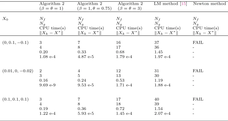
Table 6. Numerical results for Example 3.
Algorithm 2 Algorithm 2 Algorithm 2 LM method [15] Newton method (β=θ= 1) (β= 1, θ= 0.75) (β=θ= 3)
X0 Nf Nf Nf Nf Nf
Ng Ng Ng Ng Ng
CPU time(s) CPU time(s) CPU time(s) CPU time(s) CPU time(s) ∥Xk−X∗∥ ∥Xk−X∗∥ ∥Xk−X∗∥ ∥Xk−X∗∥ ∥Xk−X∗∥
(0,0.1,−0.1) 3 7 16 37 FAIL
4 8 17 36
-0.20 0.33 0.68 1.45
-1.08 e-4 4.87 e-5 1.79 e-4 1.97 e-4
-(0.01,0,−0.02) 2 4 12 31 FAIL
3 5 13 30
-0.16 0.24 0.53 1.19
-9.69 e-9 9.53 e-5 1.71 e-4 1.88 e-4
-(0.1,0.1,0.1) 3 7 17 40 FAIL
4 8 18 39
-0.19 0.36 0.72 1.54
-F(X) = {
−13 +x1+ ((5−x2)x2−2)x2= 0, −29 +x1+ ((x2+ 1)x2−14)x2= 0,
X0= (0.5,−2), X∗= (5,4).
Example 5. [23]:
F(X) = {
x1+ 1−ex2 = 0,
x1+ cosx2−2 = 0,
X0= (1.5,1.2), X∗= (1.340191857555588340...,0.850232916416951327...).
Example 6. [6]:
F(X) =
(x1−1)4ex2 = 0,
(x2−2)2(x1x2−1) = 0,
(x3+ 4)6= 0,
X0= (1,2,0), X∗= (1,2,−4). Example 7. Wood function [13]:
F(X) =
10(x2−x21) = 0,
1−x1= 0,
901/2(x
4−x23) = 0,
1−x3= 0,
101/2(x2+x4−2) = 0,
10−1/2(x
2−x4) = 0,
X0= (−3,−1,−3,−1), X∗= (1,1,1,1).
Example 8. [23]:
F(X) =
x2
1+x22+x23−x3−x23= 0,
2x1+x22−x3= 0,
1 +x1−x2x3= 0,
X0= (−1.3,−0.8,−2.4),
X∗= (−0.717018454826653767,−0.203181240635058422,−1.392754293107306018).
Example 9. n= 16, 1≤i≤n−1 [23]:
F(X) = {
xisin(xi+1)−1 = 0,
xnsin(x1)−1 = 0,
X0= (−0.85, . . . ,−0.85).
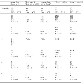
Table 7. Numerical results for Examples 4-9.
Algorithm 2 Algorithm 2 Algorithm 2 LM method [15] Newton method (β=θ= 1) (β= 1, θ= 0.75) (β=θ= 3)
Example Nf Nf Nf Nf Nf
Ng Ng Ng Ng Ng
∥Xk−X∗∥ ∥Xk−X∗∥ ∥Xk−X∗∥ ∥Xk−X∗∥ ∥Xk−X∗∥
4 13 30 102 2719 143
14 31 103 755 144
0.36 0.74 2.33 43.91 2.31
1.08 e-8 3.19 e-5 6.58 e-5 8.29 e-5 4.92 e-9
5 4 7 11 199 16
5 8 12 142 17
0.16 0.21 0.28 4.25 0.23
2.22 e-8 5.80 e-5 5.90 e-5 1.75 e-4 4.61e-9
6 1 FAIL FAIL FAIL FAIL
2 - - -
-0.08 - - -
-0 - - -
-7 55 34 39 29304 FAIL
56 35 40 6115
-1.23 0.80 0.91 336.35
-3.36 e-6 8.56 e-5 7.09 e-5 1.66 e-4
-8 7 9 12 95 28
8 10 13 78 29
0.24 0.31 0.37 2.02 0.39
6.10 e-7 3.08 e-5 3.77 e-5 1.22 e-4 4.39 e-9
9 2 8 11 27 7
3 9 12 26 8
0.23 0.51 0.64 1.31 0.29
1.54 e-5 2.08 e-5 4.34 e-5 7.01 e-5 1.76 e-9
5. Conclusions
In this paper, we proposed a regularized Newton method for unconstrained min-imization problems, and analyzed its global convergence. Convex and nonconvex problems can be solved using the presented algorithm. We also tested our algorithm on some unconstrained problems with small and medium dimensions. This algorithm does not require to calculate the step length at each iteration, and we keepαk= 1 as
algorithm and the other two methods (Newton method and Levenberg-Marquardt (LM) algorithm), the performance of Algorithm 2 in solving nonlinear equations sys-tems is also shown.
Acknowledgment
The authors are grateful for the valuable comments and suggestions of referees, which improved this paper.
References
[1] N. Andrei, Test functions for unconstrained optimization, 8-10, Averescu Avenue, Sector 1, Bucharest, Romania. Academy of Romanian Scientists, 2004.
[2] N. Andrei, An unconstrained optimization test functions collection, Adv. Model. Optim., 10
(2008), 147–161.
[3] M. Aslam Noor, K. Inayat Noor, S. T. Mohyud-Din, and A. Shabbir,An iterative method with cubic convergence for nonlinear equations, Appl. Math. Comput.,183(2006), 1249–1255. [4] K. E. Atkinson,An Introduction to Numerical Analysis, 2nd ed., John Wiley and Sons,
Singa-pore, 1988.
[5] R. L. Burden and J. D. Faires,Numerical analysis (Seventh Edition). Thomson Learning, Inc. Aug., 2001.
[6] J. E. Dennis and R. B. Schnabel,Numerical methods for unconstrained optimization and non-linear equation, 1996.
[7] T. Dehghan Niri, M. M. Hosseini, and M. Heydari,On The Convergence of an Efficient Algo-rithm For Solving Unconstrained Optimization Problems, SAUSSUREA,6(2016), 342–359. [8] E. Dolan and J. J. More ,Benchmarking optimization software with performance profiles, Math.
Program.,91(2002), 201–213.
[9] W. J. Duncan,Some devices for the solution of large sets of simultaneous linear equations (with an appendix on the reciprocation ofp artitioned matrices), The London, Edinburgh, and Dublin Philosophical Magazine and Journal of Science.,35(1944), 660–670.
[10] C. T. Kelley,Iterative methods for linear and nonlinear equations, North Carolina State Uni-versity, 1995.
[11] D. H. Li, M. Fukushima, L. Qi, and N. Yamashita, Regularized Newton methods for convex minimization problems with singular solutions, Comput. Optim. Appl.,28(2004), 131–147. [12] Y. Levina and Adi Ben-Israelb,Directional Halley and Quasi-Halley Methods in nVariables,
Inherently Parallel Algorithms in Feasibility and Optimization and their Applications.,8(2001), 345–367.
[13] J. J. More, B. S. Grabow and K. E. Hillstrom, testing unconstrained optimization software, ACM, Trans. Math. software,7(1981), 17–41.
[14] G. H. Nedzhibov, A family of multi-point iterative methods for solving systems of nonlinear equations, J. Comput. Appl. Math.,222(2008), 244–250.
[15] J. Nocedal and S. Wright,Numerical optimization, 2nd edn. Springer, New York, 2006. [16] R. A. Polyak,Regularized Newton method for unconstrained convex optimization, Math.
Pro-gram.,120(2009), 125–145.
[17] Z. Sun and K. Zhang,Solving nonlinear systems of equations based on social cognitive opti-mization, Comput. Eng. Appl.,44(2008), 42–46.
[18] F. A. Shah and M. Aslam Noor,Higher order iterative schemes for nonlinear equations using decomposition technique, Appl. Math. Comput.,266(2015), 414–423.
[19] Ch. Shen, Ch. Xiongda, and y. Liang,A regularized Newton method for degenerate unconstrained optimization problems, Optim. Lett.,6(2012), 1913–1933.
[20] J. F. Traub,Iterative Methods for the Solution of Equations, Prentice Hall, Englewood, 1964. [21] K. Ueda and N. Yamashita,Convergence properties of the regularized Newton method for the
[22] M. A. Woodbury,Inverting modified matrices, Memorandum Report 42, Statistical Research Group, Princeton NJ, 1950.
[23] X. Xiao and H. Yin,A new class of methods with higher order of convergence for solving systems of nonlinear equations, Appl. Math. Comput.,264(2015), 300–309.
![Table 1.Test problems [1, 2, 13].](https://thumb-us.123doks.com/thumbv2/123dok_us/8943409.1852777/7.612.132.476.434.612/table-test-problems.webp)