0 INTRODUCTION AND MOTIVATION
The improvement of roll dynamics is a relevant problem in vehicles with a high centre of gravity. Several roll-control systems that enhance the protection of cargo and improve roll stability have been developed. One of the most preferred roll-control solutions is anti-roll bars, which increase the stiffness of the suspension system. In this control system, torsion bars connect the left- and right-side suspensions on an axle. Active anti-roll bars can adapt to the current road conditions and lateral effects, while roll stability is improved.
Several papers propose methods to reduce the chassis roll motion of road vehicles. Three different active systems are applied: anti-roll bars, auxiliary steering angle and differential braking forces [1]. Active anti-roll bars commonly apply hydraulic actuators to achieve appropriate roll moment [2]. In
[3], an active roll-control system based on a modified suspension system is developed with the distributed control architecture. Active steering uses an auxiliary steering angle to reduce the rollover risk of the vehicle. However, this method also influences the lateral motion of the vehicle significantly [4]. The advantages of the differential braking technique are its simple construction and low cost [5]. In this case, different braking forces are generated on the wheels to reduce the lateral force. Several papers deal with the integration of the systems mentioned above. In [6], the integration of the active anti-roll bar and
active braking is presented, while [7] investigates the coordination of active control systems, which could be controlled to alter the vehicle rollover tendencies of the vehicle. The benefits of the integration of anti-roll bars and the lateral control are presented in [8]. Furthermore, the control design of anti-roll bars for the articulated vehicles is a significant and novel topic in [9]. An analysis of the snaking stability of a tractor-light trailer vehicle, in which the trailer contains anti-roll bars is presented in [10]. A special construction of semi-active anti-roll bars, which guarantees both ride and roll performances is shown in [11]. The ride and roll performances for an active anti-roll system using a PID control are analysed in [12].
The active system proposed in this paper integrates an electro-hydraulic actuator into an anti-roll bar. The system contains a high-level contanti-roller, which improves the roll dynamics of the chassis using active torque; thus, the roll motion of the chassis is influenced. The high-level control strategy is realized with a gain-scheduling Linear Quadratic (LQ) controller. The actuator of the anti-roll bar is an oscillating hydromotor with a servo valve on the low level. The actuator control guarantees the generation of the necessary active torque and satisfies the input constraint of the electric circuit. The control design is based on a constrained LQ method [13]. The goal of this paper is to demonstrate a multi-level control design of an anti-roll bar system.
The paper is organized as follows. Section 1 presents the control-oriented formulation of chassis
Design of Anti-Roll Bar Systems Based on Hierarchical Control
Varga, B. – Németh, B. – Gáspár, P. Balázs Varga1 – Balázs Németh2 – Péter Gáspár1,2,*
1 Budapest University of Technology and Economics, Department of Control for Transportation and Vehicle Systems, Hungary 2 Hungarian Academy of Sciences, Institute for Computer Science and Control, Systems and Control Laboratory, Hungary
This paper proposes the modelling and control design of active anti-roll bars. The aim is to design and generate active torque on the chassis in order to improve roll dynamics. The control system also satisfies the constraint of limited control current derived from electrical conditions. The dynamics of the electro-hydraulic anti-roll bar are formulated with fluid dynamical, electrical and mechanical equations. A linear model is derived for control-oriented purposes. Several different requirements and performances for the control influence the hierarchical handling of the control design. In the hierarchical architecture, a high level improves chassis roll dynamics via a gain-scheduling linear quadratic (LQ) control, while a low level guarantees the input limitation and produces the necessary actuator torque by a constrained LQ control. The operation of the designed anti-roll bar control system is illustrated through simulation examples.
Keywords: anti-roll bar, hydraulic actuator, gain-scheduling, LQ, automotive control application
Highlights
• Electro-hydraulic actuator modelling of an anti-roll bar system. • Constrained LQ control design for the actuator control.
roll dynamics and the electro-hydraulic actuator using fluid dynamical, electrical and mechanical equations. Section 2 describes the architecture of the active anti-roll bar control system and details the design methods of the vehicle dynamics and actuator controllers with demonstration examples. The actuation of the control system is illustrated with a simulation example in Section 3. Finally, Section 4 summarizes the contributions of the paper.
1 CONTROL-ORIENTED SYSTEM MODELLING
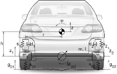
In this section, the mechanical and hydraulic equations expressing the operation of the actuator are presented. The linear vehicle model, describing the roll dynamics of the chassis is modelled, which is enhanced with the active anti-roll bar system. The actuator for this system consists of a hydromotor and a valve. The four degrees-of-freedom vehicle dynamic model is illustrated in Fig. 1.
1.1 Modelling of Chassis Roll Dynamics
Concerning the rolling motion of the chassis (sprung mass), an anti-roll bar is required so as to reduce the effect of load transfer and roll angle.
The intervention of the anti-roll bar system is a force couple on the unsprung masses, which is provided by an active torque of the electro-hydraulic actuator Mact. Lateral force Flat on the vehicle chassis and road excitations on the wheels g01, g02 are disturbances active in the system. In the model, the masses, spring stiffness, damping ratios and geometrical parameters are constants. h is the distance between the roll centre of the chassis, and its centre of gravity and r is the half-track of the vehicle. The length of the anti-roll bar arm in the longitudinal direction is denoted by aarm. In the model, the effects of the side-slip angle and under-/oversteering are ignored.
Fig. 1. Illustration of the vehicle model
The vehicle dynamics are derived from the Euler-Lagrange formalism in four second-order differential equations:
mz d d z d r d r d z d z
s s z s r s r
= −
(
+)
−(
−)
+ + −
(
+)
−(
−−
1 2 2 1 1 1 2 2
1 2 2 1
ϕ
))
ϕ+s z s z1 1+ 2 2, (1a)I d d rz d d r d rz d rz
s s rz s s
ϕ= −
(
−)
−(
+)
ϕ− + −−
(
−)
− +2 1 1 2
2
1 1 2 2
2 1 1 22
2
(
)
rϕ, (1b)m d z d r d z s z s r
s s z s g M
a z
act
1 1 1 1 1 1 1 1
1 01 1 01 01
2
= − − + + −
−
(
+)
+ +ϕ ϕ
aarm
, (1c)
m d z d r d z s z s r
s s z s g M
a z
act
2 2 2 2 2 2 2 2
2 02 2 02 02
2
= + − + − −
−
(
+)
+ −ϕ ϕ
aarm
. (1d)
The vertical dynamics of the sprung mass m, and its roll dynamics are described in Eqs. (1a) and (1b). The vertical dynamics of the unsprung masses m1, m2 are expressed in Eqs. (1c) and (1d). The proposed dynamical equations, Eq. (1) are transformed into state-space form as:
xveh=Axveh+B w1,veh veh+B u2,veh veh, (2)
where the state vector of the vehicle
xveh z z z z z z
T
=
[
1, 2, , ϕ, 1, 2, , ϕ]
incorpo-rates the vertical displacements of unsprung z1, z2 and sprung masses z, the chassis roll angle φ and their derivatives. The control input uveh = Mact of the system is the active torque generated by the electro-hydraulic actuator. The disturbances of the system
wveh g g Flat T
=
[
01, 02,]
are road excitations on thewheels and lateral forces.
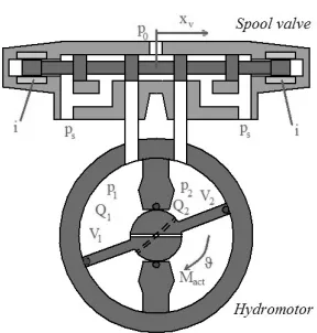
1.2 Electro-Hydraulic Actuator Model of Anti-Roll Bar System
which can be countered by the pressure difference in the two chambers provided by a pump.
The hydromotor is connected to a symmetric 4/2 four-way valve, and the spool displacement of this valve is realized by a permanent magnet flapper motor. Since the presented system has high energy density, it requires little space and has low mass. Furthermore, the actuator has a simple construction, but it requires an external high-pressure pump [14].
Fig. 2. Electro-hydraulic actuator
The physical input of the actuator is the valve current i, the output is the active torque Mact. The flapper motor and the spool can be modelled as a second order linear system, which creates a linear dependence between the valve current and the spool displacement. The motion of valve is modelled as:
1 2
2
ωv v ωv
v v v v
x D x x k i
+ + = , (3)
where kv valve gain equals k Q
p u
v N
N vmax =
∆ / 2 1
,
where QN is the rated flow at rated pressure and maximum input current, pN is the pressure drop at rated flow and uvmax is the maximum rated current. Dv is the valve damping coefficient, which can be calculated from the apparent damping ratio. Dv stands for the natural frequency of the valve [15]. Note that the modelling of the valve motion poses several difficulties. Although Eq. (3) results in a suitable form for control-oriented purposes, the null positioning of the valve is a crucial problem.
The pressures in the chambers depend on the flows of the circuits Q1, Q2. pL is the load pressure difference between the two chambers. The average flow of the system, assuming supply pressure ps is constant:
Q x p C A x p x
x p
L v L d v s v
v L
, .
(
)
=( )
−
1
ρ (4)
This equation can be linearized around (xv,0; pL,0) see [14]
QL=K x K pq v− c L, (5) where Kq is the valve flow gain coefficient and Kc is the valve pressure coefficient. In this modeling principle, the hydromotor model does not take into account the friction force and the external leakage flow. The compressibility of the fluid is considered constant [14].
The volumetric flow in the chambers is formed as:
p
V Q V c c p
L E
t L p l l L
=4
(
− + 1 − 2)
β ϑ ϑ
, (6)
where βE is the effective bulk modulus, Vt is the total volume under pressure and Vp is proportional to the areas of vane cross-sections. cl1 and cl2 are parameters of the leakage flow.
The motion equation of the shaft rotation due to the pressure difference pL and the external load Mext is:
Jϑ= −daϑ+V pp L+Mext, (7) where J is the mass of the hydromotor shaft and vanes, and da is the damping constant of the system. Mext is the effect of disturbances on the chassis roll dynamics. In the linear form, the nonlinearities of the friction are ignored.
The active torque of the actuator is determined by pL. The relationship is written as follows:
Mact =2p A aL v arm, (8)
where Av is the area of the vanes, and is the arm of the stabilizer bar in the longitudinal direction.
The control design of the actuator requires the transformation of the previous equations into a state-space form. Eqs. (3), (6) and (7) are the necessary differential equations, Eq. (5) is a part of Eq. (6):
xact =A xact act+B w1,act act+B u2,act act, (9a) yact =c xact act. (9b) The state vector of the actuator model xact xv xv p
T
= ϑ contains the spool
using Eq. (8). The control input is uact = i, while the disturbance is the external load wact = Mext.
Finally, the model of the anti-roll bar, incorporating vehicle dynamics (Eq. (2)) and actuator dynamics (Eq. (9)) is formulated as:
x Ax B w B u= + 1 + 2 , (10)
where x = [xveh, xact]T, disturbance vector is w = [wveh, wact]T , the input is u = uact and the matrices are:
A A B C
A
B B
B B B
veh veh act act
veh act =
=
=
2
1 1
1
2 2
0
0
0
0
,
, ,
,
,
,,
.
act
2 HIERARCHICAL DESIGN OF ANTI-ROLL BAR CONTROL
2.1 Performances of the Control Problem
In the previous section, the roll dynamics and the electro-hydraulic actuator were modeled, and a control-oriented model for active anti-roll bar control design was built. This section proposes the architecture and the optimal design of the control system.
The anti-roll bar control system must fulfil several requirements. The role of the system is to enhance the roll dynamics of the vehicle, which has two main components: the roll angle φ and the roll angular acceleration ϕ. First, the roll angle of the chassis influences the traveling comfort of the vehicle, and the high roll angle increases the risk of the rollover motion. Second, it is essential to take into account the roll angular acceleration, due to the impulse-like excitations. These road excitations lead to the intense angular acceleration of the chassis, while the roll angle remains small. With the minimization of ϕ, the risk of rollover caused by sudden effects can be reduced. The vehicle dynamic performances are formulated such as:
z1=ϕ z1 →min, (11a)
z2=ϕ� � � �z2 →min. (11b)
The performances z1, z2 are arranged in a vector form, such as:
z=
[
z z1 2]
T. (12)Another requirement for the control system is the minimization of the current i, for which there are two main reasons. First, there is the applied control energy,
which is an economy requirement. Since the valve has a frequent intervention, the minimization of actuation energy is necessary. Second, the current has technical limits, such as –ilimit ≤ i ≤ ilimit . Thus, the control input u = i must be minimized:
u →min u i, ≤ limit. (13) Criteria in Eqs. (11) and (13) show that the anti-roll bar system must fulfil several requirements. In the following, a cost function J, which incorporates the previous requirements, is formulated. The goal of the control design is to find a controller which minimizes the cost function:
J= z Qz u Ru dtT + T m
→
∫
1
2
0
∞
in, (14)
where Q and R are constant weights that influence the solution of the minimization problem. The role of the weights is to find a balance between the performances and the control input.
Although the design criterion (Eq. (14)) provides an adequate description of the control problem, it is difficult to find an appropriate solution. The overall formulation of the system (Eq. (10)) contains two subsystems (Eqs. (2) and (9)), whose dynamics are different: the dynamics of the chassis are slower than that of the hydraulic actuator. Moreover, the consideration of the input constraint in Eq. (13) also poses difficulties in high-order systems. It is beneficial to reduce the states of the system, which is guaranteed by the separation of the two subsystems. Furthermore, it is not necessary to constantly guarantee both of the performances (Eq. (11)). Using a changeable balance between the performances a less conservative controller can be achieved. However, it requires the reduction of the system order, which is guaranteed by the separation. In practice, dividing the optimization problem (Eq. (14)) into two sub-problems is recommended. This results in two optimal solutions to the sub-problems; however, they are suboptimal, considering the original problem.
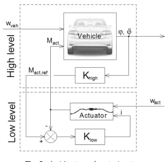
In the following, the overall system (Eq. (10)) is divided into the vehicle (Eq. (2)), and actuator (Eq. (9)) subsystems. These are the high level and the low level in the hierarchy. The input of the high-level vehicle system is the actuator torque Mact, which is the output of the low-level actuator. The interconnection between the subsystems is created by Mact.
high level in anti-roll bar is the active torque Mact. Due to economy and technical aspects, Mact must be minimized:
uveh=Mact, uveh →min. (15)
Using the control input Mact, the roll dynamic performances (Eq. (2)) must be guaranteed. However, physically, it is the output of the actuator, see (Eq. (9)). The required control input is computed with the high-level controller and is denoted by Mact,ref. The purpose of the low-level control is to guarantee the minimum error between the required and the physical torque. Thus, the next performance is formed for the low-level control design:
zact =Mact ref, −Mact zact →min. (16)
A further requirement for the control input of low-level i is defined in Eq. (13).
Based on the separation of vehicle dynamics and actuator, the optimization problem of the cost function J is divided into two parts:
min min min
K J Khigh Jveh Klow Jact
≤ + , (17)
where
Jveh=
∫
z Q z u R uT veh + vehT veh vehdt1
2
0
∞
, (18a)
Jact z Q zactT u R u dt act act T act
=1
∫
+ 2
0
∞
, (18b)
where K is the optimal controller of the problem (Eq. (14)), Khigh is the vehicle dynamic controller and Klow is the actuator controller. Note that the solution of the minimizations in Eq. (17) results in a suboptimal solution to the original minimization problem (Eq. (14)). However, in this way, a solution to the constrained optimization problem can be found. The architecture of the hierarchical control is illustrated in Fig. 3.
2.2 Vehicle Level Control Design
In the following, the control design of the high level is presented. The roll dynamic performances of the system are the minimization of the roll angle and the roll angular acceleration, see Eq. (11). A further requirement for the control system is the minimization of the control input Mact in Eq. (15). Note that it is not necessary to simultaneously guarantee all of the requirements. There are priorities among them, which depend on the current vehicle dynamic status. The priority between the performances is represented with
a scheduling variable ρveh, which is chosen as a linear combination of φ and ϕ:
ρveh
(
ϕ,ϕ)
=aϕ+bϕ, (19) where a and b are design parameters, which represent the balance between φ and ϕ. ρveh is calculated during the measurements of the roll angle and angular acceleration signals. The scheduling variable is taken into consideration in the further design of the control architecture.Fig. 3. Architecture of control system
Three criteria are defined in Section 2: the minimization of φ, ϕ and Mact. Using ρveh, different weights are defined for these criteria:
ξ ρ ξ ρ
ρ σ
i veh
m
i veh
e i
veh i i
( ) , | ( ) | , [ ; ; ],
( )
= − ≤ =
− 2
1 1 2 3 (20)
where mi and σi are scale parameters of the curves belonging to the respective criteria. ξi weights depend on ρveh, and the functions have symmetric bell curve shapes, see Fig. 4. This is adequately chosen to express the importance of each criterion at a given ρveh. Where ξi(ρveh) has a high value, the consideration of the related criterion has a high priority.
Based on the Jveh cost function minimization problem, three different LQ controllers Khigh,i i = [1; 2; 3] are designed. The resulting Khigh,i are LQ controllers computed with different Qveh, Rvehweights. • Khigh,1 operates at low roll angles and low angular
accelerations. In the absence of a critical situation, the actuator intervention is not necessary. As it saves energy, it is an economical mode of the anti-roll bar system. The weights of the LQ control design are Qveh = Rveh.
angular acceleration of the chassis increases, while the roll angle is still small. With this approach, the risk of a rollover caused by sudden effects can be reduced. The weights of the LQ control design are , Qveh > Rveh which guarantees the appropriate actuation.
• Khigh,3 has an important role in the limitation of Mact, see Eq. (16). This controller prevents the actuator from being overload. The weights of the LQ control design are Qveh < Rveh, which guarantees reduced actuation. If a common Lyapunov function Phigh of the controllers Khigh,i, then the global stability of the closed-loop systems is guaranteed [16].
a)
b)
Fig. 4. Scheduling variable dependence in high-level control; a) ξi(ρveh) functions and b) example on a Khigh element
The control strategy of the high-level control is based on the designed Khigh,i controllers and the scheduling variable-dependent ξi(ρveh) weights. In this way, a gain-scheduling LQ controller is formed:
Khigh veh K veh K veh K
veh veh
=
(
)
+(
)
+(
)
(
)
+(
)
+ξ ρ ξ ρ ξ ρ
ξ ρ ξ ρ ξ
1 1 2 2 3 3
1 2 3
(
ρρveh)
, (21)
where Khigh is the convex combination of Khigh,i. The convexity is guaranteed by the existence of Phigh and the condition | ξi(ρveh) | ≤ 1. Thus, Khigh is inside of the convex hull of Khigh,i. Fig. 4 illustrates an example
in which an element of Khigh based on Eq. (21) is computed.
2.3 Actuator Level Control Design
The torque-tracking low-level actuator design is proposed below. The controller Kact is designed based on the minimization of Jact, using the constrained LQ control method. The purpose of the controller is to guarantee the required active torque of the high-level dynamic controller and satisfy the input constraint of the low level, see Eqs (16) and (13).
The low-level LQ controller is based on a piecewise linear control strategy. This method can be used for the approximation of nonlinear systems using linear sections. Piecewise linear systems are special types of switched linear systems with state-space partition-based switching. The main difficulty in this strategy is the switching between the controllers, which can cause transients in the control system [17].
The tracking criterion in Eq. (16) of the control system requires the reformulation of the state-space equation described in Eq. (9). The plant in Eq. (9) is augmented with an integrator on signal Mact to achieve zero steady-state error. The augmented system is as follows: x z A c x z B act act act act act act act = − + 0 0 0 1, + + + = = + w B u M
A x B
act act act ref act act 2 1 0 0 1 , , ,, , , .
act actw +B uact + Mact ref 2 0
1 (22)
The LQ controller design is based on the minimization of the following cost function (Eq. (17)), which incorporates the previous conditions of Eqs. (16) and (13) and the augmented plant in Eq. (22). The weights Qact and Ract have an important role in satisfying input constraints. The minimization
min
Klow Jact problem leads to a continuous-time control algebraic Riccati equation:
P Alow act A PactT P B R B P Q low low act act Tact low act
+ − − + =
2 1
2 0
, , , (23)
where Plow is the solution to Riccati equation, Aact and
B2,act are the block matrices of Eq. (22). The optimal state feedback LQ controller Klow is derived from Plow.
It results in a conservative controller Klow with small gain, which leads to a reduced control input and the simultaneous degradation of zact tracking performance. Moreover, a large LQ gain enhances the tracking performance, but it is likely to violate the input constraint uconst. A way to guarantee (Eq. (16)) and input constraint satisfaction is presented in [13]. In this paper, an iterative LQ control design method is proposed, which yields a switching LQ controller. In the method, numerous controllers are designed using different Ract weights. The iterative function for control design is as follows:
R
u B P B
act i act i const act
T
low i act
,
,
, , , .
= ρ
(
2 −12)
(24)In this method, the different Ract,i weights are used at fixed Q matrices, ρact,i is the actual gain scaling parameter and uconst is the input constraint. Plow,i–1 is the solution of the (i – 1)th Ricatti equation (Eq. (23)).
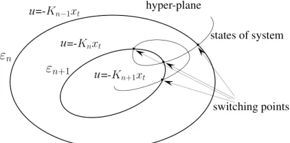
The solution to ith Riccati equation is Plow,i , from which the ith optimal LQ control can be computed. Furthermore, Plow,i determines an ellipsoidal invariant set εi in the state-space, where the input constraint can be satisfied. As a result of the iterative design, numerous LQ gains and invariant sets are computed. The controller with the largest LQ gain belongs to the smallest ellipsoid. Based on the invariant sets, a switching strategy is defined to guarantee the input constraint. In the strategy, the trajectory of xact is monitored. When the trajectory reaches the set border of an ellipsoid and moves outwards, the system switches to a more conservative controller with a smaller LQ gain. The switching function is formulated as follows:
sign(ρ(act i, )−x PactT (low i, )xact)<1. (25)
If Eq. (25) is not satisfied, then xact is out of the ith ellipsoid; thus, it is necessary to switch to the (i – 1)th controller.
Fig. 5. Invariant sets and switching of a two-state system
The solution of the switching algorithm is always the smallest ellipsoid, which contains xact. In this method, it is necessary to guarantee that xact never departs the largest ellipsoid εi. Therefore, ρact,i must be chosen sufficiently high so as to not violate this condition. Since the system states are always in the outermost invariant set, the stability of the system is guaranteed. The switching algorithm described above is illustrated in Fig. 5.
3 SIMULATION EXAMPLE
In this section, the operation of the active anti-roll bar control is presented during a simulation example. The data of the full vehicle are presented in Table 1.
Table 1. Data of vehicle and actuator models
m 1300 kg d1 4500 Ns/m d2 4500 Ns/m
I 500 kgm2 s1 50000 N/m s2 50000 N/m
r 0.8 m h 0.7 m s01 80000 N/m
aarm0.3 m ωv 7301 1/s s02 80000 N/m
kv 0.523 1/A Kq 11.02 m2 Kc 10–12 N/m
βe 6.9×10⁸ Pa Vt 1.95×10⁻⁴ m3 Vp 1.95×10⁻⁴ m3
cl1 7.85×10⁻¹⁵ m3s cl2 3.14×10⁻⁶ m3/Pa J 5 kgm2
da 1000 Ns/m Av 0.0026 m3 Dv 0.071
m1 120 kg m2 120 kg
The vehicle contains one anti-roll bar on the rear axle, which actuates to improve the roll dynamics of the vehicle.
The high-level gain-scheduling LQ control computes the currently required torque Mact,ref. The parameters in the scheduling function ρveh
(
ϕ ϕ,)
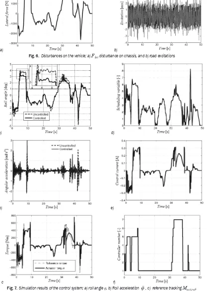
are chosen as a = 1.92 and b = 0.528. In the low-level constrained LQ control n = 7 controllers are designed. In the example, n = 1, and LQ control has the highest gain, which improves the tracking performance, while n = 7 is the most conservative, which satisfies the constraint ilimit = 0.3 A. Scheduling variable and the number of the low-level controls are chosen based on the previously defined control strategy during the simulations.a) b)
Fig. 6. Disturbances on the vehicle; a) Flat disturbance on chassis, and b) road excitations
a) d)
b) e)
c f)
the performances of the entire system Eq. (11) are guaranteed.
The required torque Mact,ref for the roll dynamics improvement by the high level control is illustrated in Fig. 7c. The changes in ρveh (Fig. 7d) guarantee the balance between φ, ϕ and Mact,ref. For example, at 20 s the disturbance Flat is around zero, and actuation is unnecessary. Therefore, ρveh has a low value. At a high Flat (e.g. 5 s to 10 s), the signal ρveh is increased to avoid extremely high Mact,ref. The operation of the low level control is evaluated based on the torque-tracking performance Eq. (15), which is guaranteed with an appropriate threshold in most of the simulation. Moreover, the control system satisfies the input constraint ilimit, see Fig. 7e. During the actuation of the current, the low level switches to the appropriate LQ control, as shown in Fig. 7f. For example, between 31 s and 39 s the current i reaches ilimit, thus the controller switches to n = 7 to avoid limit violation. However, it results in the degradation of torque tracking, see 7c.
4 CONCLUSIONS
The paper has proposed the design of anti-roll bars based on a hierarchical control architecture. The design is based on the modelling of the chassis and the electro-hydraulic actuator, in which the performance specifications and the uncertainties are formed. In the high level, the gain-scheduling LQ control is applied to design actuator torque, and the chassis roll dynamics are improved. In the low level, a constrained LQ control is applied to generate actuator torque, while the input limitation is taken into consideration. Within the hierarchical structure, the interaction between the two levels is handled. The simulation example shows that the control system improves roll dynamics and handles the input constraint simultaneously.
5 ACKNOWLEDGMENT
This paper was supported by the János Bolyai Research Scholarship of the Hungarian Academy of Sciences.
6 REFERENCES
[1] Shibahata, Y. (2005). Progress and future direction of chassis control technology. Annual Reviews in Control, vol. 29, no. 1, p. 151-158, DOI:10.1016/j.arcontrol.2004.12.004.
[2] Sampson, D., Cebon, D. (2003). Active roll control of single unit heavy road vehicles. Vehicle System Dynamics, vol. 40, no. 4, p. 229-270, DOI:10.1076/vesd.40.2.229.16540.
[3] Sampson, D., McKevitt, G., Cebon, D. (1999). The development of an active roll control system for heavy vehicles. Proceedings of 16th IAVSD Symposium on the Dynamics of Vehicles on
Roads and Tracks, p. 704-715.
[4] Odenthal, D., Bunte, T., Ackermann, J. (1999). Nonlinear steering and braking control for vehicle rollover avoidance,
Proceedings of European Control Conference.
[5] Palkovics, L., Semsey, A., Gerum, E. (1999). Rollover prevention system for commercial vehicles - additional sensorless function of the electronic brake system. Vehicle System Dynamics, vol. 32, no. 4-5, p. 285-297, DOI:10.1076/ vesd.32.4.285.2074.
[6] Gáspár, P., Szaszi, I., Bokor, J. (2004). The design of a combined control structure to prevent the rollover of heavy vehicles. European Journal of Control, vol. 10, no. 2, p. 148-162, DOI:10.3166/ejc.10.148-162.
[7] Allan, Y.L. (2002). Coordinated control of steering and anti-roll bars to alter vehicle rollover tendencies. Journal of Dynamic Systems, Measurement, and Control, vol. 124, no. 1, p. 127-132, DOI:10.1115/1.1434982.
[8] Yim, S., Jeon, K., Yi, K. (2012). An investigation into vehicle rollover prevention by coordinated control of active anti-roll bar and electronic stability program. International Journal of Control, Automation, and Systems, vol. 10, no. 2, p. 275-287,
DOI:10.1007/s12555-012-0208-9.
[9] Huang, H-H., Yedavalli, R.K. (2010). Active roll control for rollover prevention of heavy articulated vehicles with multiple-rollover-index minimization. ASME Dynamic Systems and Control Conference, DOI:10.1115/DSCC2010-4278.
[10] Šušteršič, G., Prebil, I., Ambrož, M. (2014). The snaking stability of passenger cars with light cargo trailers. Strojniški vestnik - Journal of Mechanical Engineering, vol. 60, no. 9, p. 539-548, DOI:10.5545/sv-jme.2014.1690.
[11] Stone, E.J., Cebon, D. (2008). An experimental semi-active anti-roll system. Proceedings of Institution of Mechanical Engineers, Part D: Journal of Automobile Engineering, vol. 222, no. 12, p. 2415-2433, DOI:10.1243/09544070JAUTO650.
[12] Zulkarnain, N., Imaduddin, F., Zamzuri, H., Mazlan, S.A. (2012). Application of an active anti-roll bar system for enhancing vehicle ride and handling. IEEE Colloquium on Humanities, Science & Engineering Research, DOI:10.1109/ chuser.2012.6504321.
[13] Wredenhangen, G., Bélanger, P. (1994). Piecewise-linear LQ control for systems with input constraints. Automatica, vol. 30, no. 3, p. 403-416, DOI:10.1016/0005-1098(94)90118-X.
[14] Meritt, H.E. (1967). Hydraulic Control Systems. John Wiley & Sons Inc., Hoboken.
[15] Šulc, B., Jan, J.A. (2002). Non linear modelling and control of hydraulic actuators. Acta Polytechnica, vol. 42, no. 3, p. 173-182.
[16] Boyd, S., Ghaoui, L.E., Feron, E., Balakrishnan, V. (1997).
Linear Matrix Inequalities in System and Control Theory. Society for Industrial and Applied Mathematics, Philadelphia.