A Comparison Between GA and PSO Algorithms
in Training ANN to Predict the Refractive Index
of Binary Liquid Solutions
Kamyar Movagharnejad*
and Niusha Vafaei
Faculty of Chemical Engineering, Babol Noshirvani University of Technology, Babol, Iran
(Received: 08/24/2017, Revised: 09/14/2018, Accepted: 10/04/2018) [DOI: 10.22059/JCHPE.2018.238595.1208]
Abstract
A total number of 1099 data points consisting of alcohol-alcohol, al-cohol-alkane, alkane-alkane, alcohol-amine, and acid-acid binary solu- ϐ - ϐ ȋȌǡ Ǥ ǡ ǡ ǡ - Ǥ ȋȌ ȋȌ in order to predict the refractive index of binary solutions. The op-ǦǦ ͳ͵ͳ neurons in the hidden layer, respectively. The results revealed that the ȋαͲǤͲͲ͵ͶͶͳ Ȍ ȋαͲǤͲͲͷͳͳ for test data).
Keywords
Algorithm;
ϐ Ǣ Ǣ Ǧ -tron;
-tion;
Refractive Index
Introduction
1* Corresponding Author. Tel.: 011-32334204
Email: [email protected] (K. Movagharnejad)
1. Introduction
he refractive index of a substance is de-fined as the ratio of the velocity of light in the vacuum to the velocity of light in the considered medium. This thermodynamic proper-ty depends on temperature and pressure for any pure fluid [1]. When the measurement of other thermodynamic properties is time-consuming, it is more convenient to measure the refractive in-dex [2].
The refractive index of each material is a function of temperature but this function is different for each material. The refractive index may increase or decrease with temperature which depends on the medium.
The most general form of the Lorentz–Lorenz equation which describes the refractive index is as follows:
ವమିଵ ವమାଶൌ
ସగ
ଷ ܰߙ (1)
where ݊ is the refractive index, is the number
timates for liquids, solids and homogeneous sol-ids.
For many gases the square of the refractive index is݊ଶൎ ͳ, so this equation reduces to:
݊ଶെ ͳ ൎ Ͷߨܰߙ (2)
Or simply:
݊ െ ͳ ൎ ʹߨܰߙ (3)
This applies to gases at ordinary pressures. The refractive index of the gas may be expressed in terms of the molar refractivity as:
݊ ൎ ටͳ ଷோ் (4)
where P is the pressure of the gas, R is the universal gas constant, and T is the absolute temperature. These parameters determine N which is the number density [3]. It is known that the refractive index for most glasses increases with temperature, while for plastic polymers, the opposite is true. The refractive index of water decreases with temperature. The decrease in the refractive index of most organic liquids with tem-perature is usually greater than water [4].
Refractive index has many applications, but the most important one may be the identification or concentration measurement of a specific sub-stance. Generally, the refractive index is used to measure the concentration of solutes in aqueous solutions. For instance, in an aqueous sugar solu-tion, the refractive index may be used to deter-mine the sugar content (Brix degree), also it may be used to determine the drug concentration in the pharmaceutical industry. Another application of the refractive index may be the estimation of thermo-physical properties of hydrocarbons and petroleum mixtures [5].
Some empirical equations have been used to pre-dict the refractive index. The relationship be-tween refractive index, density and other physical properties of hydrocarbons investigated was by Lipkin and Martin:
݊ ൌ
ͻǤͺͺ݀ െ ͲǤͶͲͶͶܣ݀ െ ͲǤͻܣ ͳ͵Ǥͷ ͷǤͷͶ͵݀ െ ͲǤͶܣ ͳʹǤͺ͵ (5)
where ୈ is the refractive index at ʹͲԨ for the D
line of sodium, is the density at ʹͲԨ and is
െͳͲହൈ temperature coefficient of density (Ƚሻ,
which is obtained from the approximate molecu-lar weight [6].
The relation between refractive index with sur-face tension was introduced by Deetlefs for ionic liquids as below:
ߪభరൌ ቀ ோቁ ቀ
ವమିଵ
ವమାଶቁ (6)
where ୈ is the refractive index, is the
para-chor, a surface-tension-weighted molar volume, and ୫ is the molar refraction [7].
Sattari and his colleagues developed a based-group contribution method to predict the refrac-tive indices of ionic liquids and they observed that the refractive index is a linear function of the temperature.
݊ൌ ܣ ܤܶ (7)
ܣ ൌ ͳǤͷͲͺʹ σୀଵ݊ǡܽ (8) ܤ ൌ െͳǤͶʹͲ ൈ ͳͲିସ σ ݊
ǡܾ
ୀଵ (9)
where ݊ is the number of occurrences of the ith
functional group of anions and cations, k is the total number of different functional groups of the anions and cations, and ܽ and ܾ are the relevant
coefficients of the ith functional group [8].
There are numerous empirical equations based on experimental measurements for the prediction of the refractive index but these correlations have certain limitations. They usually include a large number of coefficients for each equation, require a separate equation for each temperature and they are not able to predict several parameters simultaneously. Recently, intelligent modeling techniques such as the artificial neural network (ANN) are successfully used to predict the differ-entthermophysical properties. The most im-portant characteristic of the neural network models is their flexibility to predict the nonlinear behavior of chemical properties and their ability to estimate any function with high dimensional data. The mechanism of the ANN models is to construct relationships between the input and output data and predict the properties with reasonable accuracy [9, 10]. Recently, ANN mod-els have been used to predict different thermody-namic properties such as viscosity, density, elec-trical conductivity, porosity, hardness and so on [11-18].
algorithm such as the ANN is a vital step in this computational procedure.
Although the refractive index of some pure and a few mixtures was reported in the literature, these limited experimental data still cannot satisfy the requirements for their wide applications. Besides, experimental measurements are time-consuming and relatively expensive and are not always available, so estimation methods have been wide-ly used instead of the rare experimental data [20]. The main purpose of this work is to develop a predictive model for the refractive index of binary mixtures. Specifically, it defines the best neural architecture using the ANN along with the pa-rameters correlated with it, and it predicts the refractive index of the studied systems from the calculated empirical parameters.
For better response, the neural network trained by genetic (GA) and particle swarm optimization algorithm (PSO) independently.
2. Theory
In this section, the techniques of ANN, GA and PSO are briefly presented.
2.1. Artificial neural network algorithm (ANN)
The applicability of ANN in process industries and scientific research has been growing contin-uously in recent years [21]. Given adequate ex-perimental data, the ANN model is able to approx-imate any continuous function with a satisfactory accuracy. The adequate performance of an ANN depends on several main elements. The first ele-ment is related to the collection of the input and output data. The second element is the type of the network architecture. Different network architec-tures may result in different estimations with varying degrees of accuracy. The third element is the model size and the problem complication. The model size and the problem complication have to be proportional to each other and the last ele-ment is related to the network training. In this paper like many other research papers in ANN modeling, the focus is on this last item [22]. ANN is a non-linear learning mathematical model that follows the human brain procedures. This technique is used in various scientific and
engi-neering areas including prediction of physical and chemical properties. The input data is moved across any two successive layers and in each layer, the data is weighted and then passed to the next layer through a proper transfer function. In the training stage, the ANN revises the weights and biases of each neuron [19].
Gradient descent algorithms such as Back-Propagation (BP) method are used by many re-searchers in recent years. These rere-searchers have included some of the advantages of these meth-ods such as adequate implementations, better fine-tuning, and quicker convergence. However, some other researchers have listed the disad-vantages of these methods such as involving in local minima and ill performances. So the com-mon gradient search method is may be trapped in local optima. This is however not the case for Evolutionary Algorithms (EAs) which have better chances to reach the global optimal [22]. On the other hand, these algorithms are suitable for complicated problems [23]. Many different at-tempts have been tried by several researchers to solve this problem including imposing constraints on the search area, restarting training, adjusting training parameters, and reconstruction of the ANN architecture [24]. One of the most successful methods is to make use of EAs such as PSO, and GAs to train the ANNs. PSO or GA are global search algorithms and are more appropriate for local minima problems [25, 26].
When these algorithms are applied to neural networks, they find the best neural network ar-chitecture, optimizing the neural network learn-ing parameters, and weights. In this way, emer-gence EAs and ANN may improve the predictive power of simple ANN, PSO or GA models [22].
2.2. Genetic algorithm (GA)
genera-tions, only the better individuals will survive. In general, GA may be applied to a wide range of optimization problems. GA was created to solve sequential decision processes but recently, it has been applied widely in both optimization and learning problems [28, 29]. The two main sub-jects in searching strategies for optimization problems are: exploiting the best solution and discovery of the search area [30, 31]. GA makes a balance between these two main subjects and also avoids the local minima. Fundamentally, the operation of weights evolution using GA belonged to the number of populations and generations. If these parameters were set nominal, the evolution may converge to a premature solution. However, the larger number of populations and generations would require longer convergence times [32]. The steps of GA to reach the optimum connection weights of ANN may be listed as follows:
At the first step, the primary population of ran-dom weights was generated to create the original ANN. Then theANN was improved using the pop-ulation weights by computing the training error. At the next section parents for genetic manipula-tion were selected and a new populamanipula-tion of weights was constructed.
At the last section,the most appropriate popula-tion of weights was designated as the sequel of the performed GA, for the weights evolved using GA. The procedure may be terminated when the number of generation reaches a certain number [33].
Since the back propagation error algorithm is too slow, GA may be used to select the primary weight. In other words, by a combination of neu-ral network with GA, the performance of the re-sults may increase. In this research, in both train-ing and testtrain-ing data, GA was used to optimize the basic ANN behavior.
2.3. Particle swarm optimization (PSO)
PSO is a global optimization method introduced by Eberhart and Kennedy [33, 34]. The funda-mental motivation of PSO algorithm was the so-cial natural phenomena, such as flocks of birds and schools of fish in order to direct swarms of particles towards the most promising search ar-ea. PSO has shown a good performance in static optimization problems. In this method, a
popula-tion of individuals is exploited to find the promis-ing regions of the search area. In this study, we call the population a swarm and the individuals are called particles. Each particle in the swarm may be considered as a candidate solution. Each particle may move with a compatible velocity through the search area. These particles adjust their positions according to their own experience and also the experience of the neighboring parti-cles. The mutual effect may be described as the fly of the particles towards the global minimum [35-37]. A predefined function describes the close-ness of particles to the global minimum. In this research, a particle demonstrates the weight vec-tor of ANNs, including biases. The dimension of the search area may be defined as the total num-ber of weights and biases [22].
The PSO procedure can be described as follows. At first, a population size, locations, and velocities of factors, and the number of weights and biases were initialized. Then, the current best fitness attained by particle p was set as ௦௧ .The ௦௧
with the best value was set as ݃௦௧ and stored.
Subsequently, the agreeable optimization fitness function fp was evaluatedfor each particle as the Mean Square Error (MSE). Then, the evaluated fitness value fp of each particle was contrasted with its ௦௧ value. If ݂ ൏ ܾ݁ݏݐǡthen ܾ݁ݏݐ ൌ ݂ andܾ݁ݏݐݔ ൌ ݔ. where xp stands for the current coordinates of particle p, and the best xp stands for the coordinates corresponding to the best fitness of particle p. The objective function value was obtained for new locations of each particle. If a better position was obtained,
ܾ݁ݏݐ value was replaced. As in Step 1, ݃௦௧
val-ue was selected among ௦௧ values. If the new ݃௦௧ value was better than the previous one, the ݃௦௧value was replaced. If ݂ ൏ ܾ݃݁ݏݐ then ݃௦௧ ൌ , where ݃௦௧ is the particle having the
overall best fitness over all particles in the swarm. The velocity and location of the particle may change due to the Eqs. 9 and 10, respectively [14, 19].Then each particle p may flyaccording to Eq. 10. If you reach the maximum number of iter-ations, the procedure would be terminated; oth-erwise the procedure was looped to step 3 until convergence.
where acc stands for the acceleration constant, and rand returns a uniform random number be-tween 0 and 1.
ൌ (11)
ܸis the current velocity, ܸί1 is the former
veloci-ty, xp is the present particle location, xpp is the former particle location, and i is the particle in-dex. In the last step the coordinates bestxp and
best x݃௦௧are used to find the global minimum.
Similarly, the PSO algorithm was also applied to obtain the initial weights of the neural network. The inputs are the initial weights that should be
calculated and the output is the summation of errors that should be minimized.
2.4. Data bank
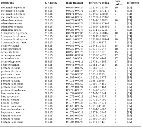
Since this research is purely computational, all the data (experimental) needed for the calcula-tions were taken from literature [38-46]. A total number of 1099 experimental data points for the refractive index were gathered in which the de-tails are presented in Table 1, including the tem-perature range, mole fraction range, refractive index range, number of data points and the refer-ences.
Table 1. Name and specification of compounds
compound T/K range mole fraction refractive index data points reference
methanol+n-pentane 298.15 0.0464-0.9734 1.3274-1.35359 10 [33]
methanol+n-hexane 298.15 0.0532-0.9771 1.32871-1.77118 11 [33]
methanol+n-heptane 298.15 0.0171-0.9765 1.32993-1.3838 9 [33]
methanol+n-octane 298.15 0.0367-0.9853 1.32962-1.39465 8 [33]
ethanol+n-pentane 298.15 0.0673-0.9174 1.3541-1.35823 10 [33]
ethanol+n-hexane 298.15 0.0569-0.9673 1.35988-1.37167 9 [33]
ethanol+n-heptane 298.15 0.0831-0.9744 1.36044-1.38382 9 [33]
ethanol+n-octane 298.15 0.0986-0.9773 1.3611-1.39295 9 [33]
1-propanol+n-pentane 298.15 0.0291-0.9586 1.35502-1.38162 10 [33]
1-propanol+n-hexane 298.15 0.1148-0.9594 1.37249-1.3823 9 [33]
1-propanol+n-heptane 298.15 0.0919-0.967 1.38398-1.38441 10 [33]
1-propanol+n-octane 298.15 0.1018-0.9677 1.385-1.39375 9 [33]
octane+ethanol 298.15 0.0686-0.9212 1.3641-1.3939 18 [34]
octane+propanol 298.15 0.0237-0.9245 1.3835-1.3943 18 [34]
octane+butanol 298.15 0.0453-0.9376 1.3948-1.397 15 [34]
octane+pentanol 298.15 0.0189-0.9457 1.3955-1.4075 17 [34]
octane+hexanol 298.15 0.0515-0.959 1.3956-1.4147 17 [34]
octane+heptanol 298.15 0.0616-0.9111 1.3971-1.4205 17 [34]
octane+octanol 298.15 0.0641-0.9635 1.3961-1.4257 16 [34]
pentane+hexane 298.15 0.1045-0.8997 1.3569-1.3715 9 [35]
pentane+heptane 298.15 0.1046-0.8929 1.359-1.3826 9 [35]
pentane+octane 298.15 0.1059-0.9035 1.361-1.3925 9 [35]
pentane+nonane 298.15 0.1995-0.904 1.3626-1.3975 8 [35]
pentane+decane 298.15 0.1031-0.9008 1.365-1.4068 9 [35]
pentane+undecane 298.15 0.0962-0.8967 1.3805-1.4152 9 [35]
pentane+dodecane 298.15 0.1094-0.8991 1.3684-1.4164 9 [35]
pentane+hexadecane 298.15 0.3099-0.9029 1.3747-1.4233 7 [35]
hexane+heptane 298.15 0.1059-0.8993 1.3745-1.3841 9 [35]
hexane+octane 298.15 0.1072-0.9018 1.3761-1.3937 9 [35]
hexane+nonane 298.15 0.1073-0.9035 1.3772-1.4009 9 [35]
hexane+decane 298.15 0.1074-0.9036 1.3788-1.4074 9 [35]
hexane+dodecane 298.15 0.1128-0.9037 1.381-1.4168 9 [35]
hexane+hexadecane 298.15 0.1046-0.9026 1.3864-1.4306 9 [35]
heptane+octane 298.15 0.1073-0.9012 1.3873-1.3945 9 [35]
heptane+nonane 298.15 0.1102-0.8996 1.3875-1.4021 9 [35]
heptane+decane 298.15 0.0985-0.903 1.3886-1.4086 9 [35]
compound T/K range mole fraction refractive index data points reference
heptane+dodecane 298.15 0.1076-0.9039 1.3907-1.4174 9 [35]
heptane+hexadecane 298.15 0.167-0.9019 1.3946-1.4316 9 [35]
octane+nonane 298.15 0.1092-0.9025 1.3963-1.4027 9 [35]
octane+decane 298.15 0.2142-0.9058 1.3968-1.4027 9 [35]
octane+undecane 298.15 0.1011-0.9039 1.3975-1.4132 9 [35]
octane+dodecane 298.15 0.1117-0.9048 1.3982-1.4177 9 [35]
octane+hexadecane 298.15 0.1039-0.9049 1.4015-1.4308 9 [35]
nonane+decane 298.15 0.1051-0.897 1.4043-1.4093 9 [35]
nonane+undecane 298.15 0.1034-0.9038 1.4045-1.4136 9 [35]
nonane+dodecane 298.15 0.0957-0.9023 1.4054-1.4183 9 [35]
nonane+hexadecane 298.15 0.1105-0.8988 1.4084-1.4323 9 [35]
decane+undecane 298.15 0.1074-0.9056 1.4105-1.4148 9 [35]
decane+dodecane 298.15 0.1071-0.9045 1.4115-1.419 9 [35]
decane+hexadecane 298.15 0.151-0.9041 1.417-1.4328 9 [35]
undecane+dodecane 298.15 0.106-0.9084 1.4156-1.4192 9 [35]
undecane+hexadecane 298.15 0.1095-0.9031 1.4182-1.4331 9 [35]
dodecane+hexadecane 298.15 0.1077-0.905 1.4218-1.4331 9 [35]
hexadecane+1-butanol 298.15-318.15 0.0903-0.9628 1.396-1.4347 30 [36]
hexadecane+1-pentanol 298.15 0.0831-0.9314 1.4101-1.4345 10 [36]
hexadecane+1-hexanol 298.15 0.0791-0.9184 1.4105-1.4347 10 [36]
hexadecane+1-heptanol 298.15 0.0893-0.9242 1.4123-1.4346 10 [36]
heptadecane+1-butanol 298.15 0.0867-0.9379 1.3996-1.4357 10 [36]
heptadecane+1-pentanol 298.15 0.1472-0.898 1.4103-1.4357 10 [36]
heptadecane+1-hexanol 298.15 0.0961-0.9107 1.4189-1.4356 10 [36]
heptadecane+1-heptanol 298.15 0.305-0.9194 1.4268-1.4357 8 [36]
methanol+2methyl,1butanol 298.15 0.0485-0.9503 1.33618-1.40702 19 [37]
ethanol+2methyl,1butanol 298.15 0.0486-0.9503 1.36358-1.40734 18 [37]
propanol+2methyl,1butanol 298.15 0.051-0.949 1.38483-1.40768 19 [38]
propanol+3methyl,1butanol 298.15 0.05-0.95 1.38458-1.40447 19 [38]
heptanoic acid+propanoic acid 293.15-313.15 0.0539-0.95 1.3816-1.4223 55 [39]
heptanoic acid+butanoic acid 293.15-313.15 0.0559-0.9575 1.392-1.4226 55 [39]
1-Propanol+ dicyclohexylamine 288.15-323.15 0.0527-0.9491 1.38876-1.48522 88 [40]
1-butanol+ dicyclohexylamine 288.15-323-15 0.0512-0.9493 1.39701-1.48502 88 [40]
1-pentanol+dicyclohexylamine 288.15-323.15 0.0525-0.9495 1.40539-1.48486 88 [40]
2.5. Criteria assessment of models
The statistical parameters such as the mean squared error (MSE) and the coefficient of deter-mination (ܴଶ) and the average absolute relation
deviation (AARD) is applied for the performance assessment and to identify the accuracy of the developed ANN models which are defined as fol-lows:
Mean squared errors:
ൌͳሺห୮୰ୢǡ୧െ ୣ୶୮ǡ୧หሻଶ
୧ୀଵ (12)
Average absolute relative deviations:
Ψ ൌͳͲͲ ห୮୰ୢǡ୧െ ୣ୶୮ǡ୧ห ୣ୶୮ǡ୧
୧ୀଵ (13)
Squared correlation coefficients:
ଶൌ ͳ െσ ሺ୧ୀଵ ୮୰ୢǡ୧െ ୣ୶୮ǡ୧ሻ
σ ሺ୧ୀଵ ୮୰ୢǡ୧െ ୫ሻ (14)
where ݕௗǡis the predicted value using the ANN
model, ݕ௫ǡis the experimental value, N is the
number of data, and ݕ is the average of the
ex-perimental value.
3. Results and Discussions
3.1. Model structure
Before performing the ANN training stage, a data set is obtained from the literature [33-41]. There is a difference in magnitude and dimension of experimental data, therefore it should be normal-ized before being training stage. Manifold ANN structures were considered to choose the most accurate architecture. The optimal number of neurons was specified by trial and error.
The effectiveness of ANN in training stage must improve with augmenting the number of neurons, while the effectiveness of ANN in testing stage results in optimum value at an optimal number of hidden neurons. After training the ANN success-fully, the trained network model was used to pre-dict the testing data set and the comparison of the predicted and experimental data was carried out. The trained model was then assumed successful if the model would have given good outcomes for the testing data set. As mentioned above, the ANN training was started with 1 neuron in the hidden layer and piecemeal the neuron number in-creased.
The architecture consists of one input layer fol-lowed by a hidden layer and an output layer. Aside from temperature, the mole fraction of the first component and molecular weights, the input set consists of 6 functional groups of CH3, CH2, CH, OH, NH and COOH. The optimal number of neu-rons was determined according to the lowest AARD%. The optimal ANN-GA consisted of 13 neurons in the hidden layer and the optimal ANN-PSO consisted of 16 neurons in the hidden layer. Thus, the best ANN topology was attained as (10-13-1) for ANN-GA and (10-16-1) for ANN-PSO.
3.2. ANN-GA model
The combination of ANN and GA was used. This means that the weights of the neural network were determined using GA. First, the structure of the neural network should have been determined by the user. That was the number of neurons. Then, the neural network weights were deter-mined by using a GA. The GA is capable to opti-mize and miniopti-mize an objective function, which here should be minimized, is the difference be-tween the actual data and output data of a neural network. This means that, at any stage, weight coefficients were selected and neural network output was calculated, and its difference with the actual data was obtained, which in fact was the
objective function value. In Fig. 2 the Objective function (MSE) is drawn by max generations.
Figure 2. Objective function with the number of genera-tions for ANN-GA model
We inserted 1099 refractive indices in the data-base, trained, validated and tested the network, and then, according to the output obtained after optimization of the weights by GA, the neural network is better trained. As a result, the refrac-tive index that was predicted is very close to the actual refractive index. Figs. 3, 4 and 5 show the results of applying this algorithm for train and validation test data:
Figure 3. Experimental and Predicted Train Data for ANN-GA model
Figure 5. Experimental and Predicted Test Data for ANN-GA model
3.3. ANN-PSO
In this section, the particle swarm optimization algorithm was used to optimize the weights of the neural network to predict the refractive index of binary solutions. At this stage, 1099 refractive indices of the database were used. Figs. 6, 7 and 8 show that the actual data and the model predic-tions are in good agreement with each other. The results are given in the Tables 2 and 3.
Table 2. Results of prediction of binary solutions refrac-tive indices using ANN-GA with 10-13-1 structure
Data-set
Classi-fication MSE AARD% R2
Train 0.0050181 8.2123 0.9091
Validation 0.0059107 2.4611 0.9851
Test 0.005117 1.4103 0.9884
Figure 6. Experimental and Predicted Train Data for ANN-PSO model
Table 3. Results of prediction of binary solutions refrac-tive indices using ANN-PSO with 10-16-1 structure
Data-set
Classification MSE AARD% R2
Train 0.003836 7.9552 0.9944
Validation 0.003535 1.6643 0.9843
Test 0.003441 1.4024 0.9852
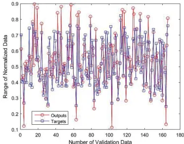
Figure 7. Experimental and Predicted Validation Data for
ANN-PSOmodel
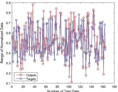
Figure 8. Experimental and Predicted Test Data for ANN-PSO model
4. Conclusions
gathered from the published scientific literature. Temperature, the molecular weight of the pure components, the mole fraction of one component and 6 structural groups of the components were adapted as input parameters of the multi-layer perceptron neural network. The ANN-GA and ANN-PSO methodology have been compared with each other. The convergence performance and prediction accuracy of the PSO-based ANN are much better (MSE= 0.003441) than the GA based ANN (MSE=0.005117).
Acknowledgment
The authors acknowledge the funding support of the Babol Noshiravani University of Technology through Grant Program No. BNUT/370675/97.
References
[1] Riazi, M. R. and Roomi, Y. A. (2001). “Use of the Refractive Index in the Estimation of Ther-mophysical Properties of Hydrocarbons and Pe-troleum Mixtures.” Industrial & Engineering Chemistry Research, Vol. 40, No. 8, pp. 1975-1984. [2] Ali, A. and Tariq, T. (2008). “Deviations in re-fractive index parameters and applicability of mixing rules in binary mixtures of benzene +1, 2-dichloroethane at different temperatures.”
Chemical Engineering Communications, Vol. 195, No.1, pp. 43–56.
[3] Lorentz, A. H. (1881). “Ueber die Anwendung des Satzes vom Virial in der kinetischen Theorie der Gase.” Wiedemanns Annalen (Annalen der Physik), Vol. 248, No. 1, pp. 127–136.
[4] Tropf., W. J., Thomas, M. E. and Harris, T. J. (1995). Handbook of Optics. 2nd ed. Vol. 2,Chapter 33, McGraw-Hill, New York.
[5] Koohyar F. J. (2013). “Refractive Index and Its Applications.” Journal of Thermodynamics & Ca-talysis, Vol.4, No.2.
[6] Lipkin, M. R. and Martin, C. C. (1946), “Equa-tion Relating Density, Refractive index, and Mo-lecular Weight for Paraffins and Naphthenes.”
Industrial and Engineering Chemistry, vol. 18, No. 6. pp. 380-382.
[7] Deetlefs, M., Seddon, K.R. and Shara, M. (2006). “Predicting of Physical Properties of Ionic
Liquids.” Physical Chemistry Chemical Physics, Vol.8, No. 5, pp. 642-649.
[8] Sattari, M., Kamari, A., Mohammadi, A.H. and Ramjugernath, D. (2014). “A group contribution method for estimating the refractive indices of ionic liquids.” Molecular Liquids, Vol. 200, Part B, pp. 410-415.
[9] Moosavi, M. and Soltani, N. (2013). “Prediction of hydrocarbon densities using an artificial neural network–group contribution method up to high temperatures and pressures.” Thermochimica Acta, Vol. 556, pp. 89-96.
[10] Lashkarblooki, M., Hezave, A. Z., Al-Ajmi, A. M. and Ayatollahi, S. (2012). “Viscosity prediction of ternary mixtures containing ILs using multi-layer perceptron artificial neural network.” Fluid Phase Equilibria Vol. 326, pp.15-20.
[11] Ozerdem, M. S. (2008). “Artificial neural network approach to predict the electrical con-ductivity and density of Ag–Ni binary alloys.”
Journal of Materials Processing Technology, Vol. 208, No. 1-3, pp. 470-476.
[12] Griffin, W. O. and Darsey, J. A. (2013). “Artifi-cial neural network prediction indicators of den-sity functional theory metal hydride models.” In-ternational Journal of Hydrogen Energy, Vol. 38, No. 27, pp. 11920-11929.
[13] Hassan, A. M., Alrashdan, A., Hayajneh, M.T. and Mayyas, A.T. (2009). “Prediction of density, porosity and hardness in aluminum–copper-based composite materials using artificial neural network.” Journal of Materials Processing Tech-nology, Vol. 209, No. 2, pp. 894-899.
[14] Torkar, D., Novak, S. and Novak, F. (2008). “Apparent viscosity prediction of alumina– paraffin suspensions using artificial neural net-works”, Journal of Materials Processing Technolo-gy, Vol. 203, No. 1-3, pp. 208-215.
[15] Ghaderi, F., Ghaderi, A. H., Najafi, B. and Gha-deri, N. (2013). “Viscosity prediction by computa-tional method and artificial neural network ap-proach: The case of six refrigerants.” The Journal of Supercritical Fluids, Vol. 81, pp. 67-78.
132 K. Movagharnejad and N. Vafaei / Journal of Chemical and Petroleum Engineering, 52 (2), December 2018 / 123-133
[17] Salam, M., Al-Alawi, S. and Maqrashi, A. (2008). “Prediction of equivalent salt deposit density of contaminated glass plates using artifi-cial neural networks.” Journal of Electrostatics, Vol. 66, pp. 526-530.
[18] Ahmadi, S. H., Sepaskhah, A. R., Andersen, M.N., Plauborg, F., Jensen, C. R. and Hansen, S. (2014). “Modeling root length density of field grown potatoes under different irrigation strate-gies and soil textures using artificial neural net-works.” Field Crops Research. Vol. 162, pp. 99-107. [19] Ghaedi, A. (2015). “Simultaneous prediction of the thermodynamic properties of aqueous so-lution of ethylene glycol monoethyl ether using artificial neural network.” Journal of Molecular Liquids, Vol. 207, pp.327-333.
[20] Soriano, A. N., Ornedo-Ramos, K. F. P., Muriel, C. A. M., Adornado, A. P., Bungay, V. C., & Li, M. H. (2016). “Prediction of refractive index of binary solutions consisting of ionic liquids and alcohols (methanol or ethanol or 1-propanol) using artifi-cial neural network”, Journal of the Taiwan Insti-tute of Chemical Engineers, Vol.65, pp. 83-90. [21] Sexton, R. S., Dorsey, R. E. and Sikander, N.A. (2002). “Simultaneous optimization of neural network function and architecture algorithm.”
Decision Support Systems, pp. 1034-1047.
[22] Braik M., Sheta A. and Arieqat A. (2008). "A comparison between GAs and PSO in training ANN to model the TE chemical process reactor." In AISB 2008 Convention communication, interac-tion and social intelligence, Vol. 11, p. 24-30. [23] Fogel, D. B. (1994). “An introduction to simu-lated evolutionary optimization.” IEEE Transac-tions on Neural Networks, Vol. 5, No. 1, pp. 3-14. [24] Huang, Y. (2009). “Advances in Artificial Neural Networks – Methodological
Development and Application”, Algorithms. Vol. 2, No. 3, pp.973-1007.
[25] Abbass, H. A., Sarker, R. and Newton, C. (2001). “PDE: A Pareto-frontier Differential Evo-lution Approach for Multi-objective Optimization Problems.” in Proceedings of the Congress on Evo-lutionary Computation 2001 (CEC’2001), Vol. 2, pp. 971–978, Piscataway, New Jersey, IEEE Service Center.
[26] Kiran, R., Jetti, S. R. and Venayagamoorthy, G. K. (2006). ‘Online training of generalized neuron with particle swarm optimization’, in Interna-tional Joint Conference on Neural Networks, IJCNN 06, Vancouver, BC, Canada, pp. 5088– 5095. IEEE, (2006).
[27] Choenauer, M. and Michalewicz, Z. (1997). “Evolutionary computation control and cybernet-ics.” Proceedings of the IEEE, Vol. 26, No. 3, pp. 307–338.
[28] Sit, C. W. (2005). “Application of Artificial Neural Network-Genetic Algorithm in Inferential Estimation and Control of a Distillation Column”, ME thesis, Faculty of Chemical and Natural Re-sources Engineering, Universiti Teknologi Malay-sia.
[29] Sheta, A. and Turabieh, H. (2006). “A com-parison between genetic algorithms and sequen-tial quadratic programming in solving con-strained optimization problems”, ICGST International Journal on Artificial Intelligence and Machine Learning, Vol. 6, No. 1, pp. 67–74.
[30] Gen, M. and Cheng, R. (1997). Genetic Algo-rithms and Engineering Design, John Wiley & Son, Inc., Hoboken.
[31] Sheta, A., Turabieh, H. and Vasant, P. (2007). “Hybrid optimization genetic algorithms (HOGA) with interactive evolution to solve constraint op-timization problems.” International Journal of Computational Science, Vol.1, No. 4, pp. 395–406. [32] Sheta A. and Eghneem, K. (2007). “Training artificial neural networks using genetic algo-rithms to predict the price of the general index for Amman stock exchange”, in Midwest Artificial Intelligence and Cognitive Science Conference, DePaul University, Chicago, IL, USA, Vol. 92, pp. 7– 13.
[33] Kennedy, J. and Eberhart, R. C. (1995). “Par-ticle swarm optimization’, Proceedings of IEEE International Conference on Neural Networks (Perth, Australia), IEEE Service Center, Pisca-taway, NJ, Vol. 5, No. 3, pp. 1942–1948.
[34] Kennedy, J., Eberhart, R. C. and Shi, Y. (2001).
Swarm Intelligence, Morgan Kaufmann Publish-ers, San Francisco.
Interna-133 K. Movagharnejad and N. Vafaei / Journal of Chemical and Petroleum Engineering, 52 (2), December 2018 / 123-133
tional Joint Conference on Neural Networks, IJCNN 06, Vancouver, BC, Canada, pp. 5088– 5095. IEEE.
[36] Richer, T.J. and Blackwell, T.M. (2006). “When is a swarm necessary?”, in Proceedings of the 2006 IEEE Congress on Evolutionary Compu-tation, eds., Gary G. Yen, Simon M. Lucas, Gary Fogel, Graham Kendall, Ralf Salomon, Byoung-Tak Zhang, Carlos A. Coello, and Thomas Philip Runarsson, pp. 1469–1476, Vancouver, BC, Cana-da, IEEE Press.
[37] Kwok, N., Liu, D. and Tan, K. (2006). “An em-pirical study on the setting of control coefficient in particle swarm optimization”, in Proceedings of IEEE Congress on Evolutionary Computation (CEC 2006), Vancouver, BC, Canada, pp. 3165– 3172, Vancouver, BC, Canada, IEEE Press.
[38] Orge, B., Iglesias, M., Rodriguez, A., Canosa, J. M. and Tojo. J. (1997) “Mixing properties of (methanol, ethanol, or 1-propanol) with (n-pentane, n-hexane, n-heptane and n-octane) at 298.15 K.” Fluid Phase Equilibria, Vol. 133, No. 1-2, pp. 213-227.
ȏ͵ͻȐ Ǥǡ Ǥǡ ǡ Ǥ Ǥǡ Ç-Prez, M., Oscar, C., Cabanas, M. and Jimenez. E. (2003). “Density, Surface Tension, and Refractive Index of Octane + 1-Alkanol Mixtures at T = 298.15 K.”
Journal of Chemical & Engineering Data, Vol. 48, No. 5, pp.1251-1255.
[40] Aucejo, A., Burguet, A. C., Munoz, R. and Marques, J.L. (1995). “Densities, Viscosities, and Refractive Indices of Some n-Alkane Binary Liq-uid Systems at 298.15 K.” Journal of Chemical and Engineering Data, Vol. 40, No. 1, pp. 141-147. [41] Mehra, R. (2003). “Application of refractive index mixing rules in binary systems of hexade-cane and heptadehexade-cane with n-alkanols at different temperatures.” Journal of Chemical Sciences. Vol. 115, No. 2, pp. 147–154.
[42] Resa, J. M., Gonzalez, C. and Goenaga, J. M. (2005). “Density, Refractive Index, Speed of Sound at 298.15 K, and Vapor-Liquid Equilibria at 101.3 kPa for Binary Mixtures of Methanol + butanol and Ethanol + 2-Methyl-1-butanol.” Journal of Chemical & Engineering Data, Vol. 50, No. 5, pp.1570-1575.
[43] Resa, J.M., Gonzalez, C. and Goenaga, J. M. (2006). “Density, Refractive Index, Speed of Sound at 298.15 K, and Vapor-Liquid Equilibria at 101.3 kPa for Binary Mixtures of Propanol + 2-Methyl-1-butanol and Propanol + 3-Methyl-1-butanol.” Journal of Chemical & Engineering Data, Vol. 51, Vol. 1, pp. 73-78.
[44] Bahadur, I., Naidoo, P., Singh, S., Ramjuger-nath, D. and Deenadayalu, N. (2014). “Effect of temperature on density, sound velocity, refractive index and their derived properties for the binary systems (heptanoic acid + propanoic or butanoic acids)”, The Journal of Chemical Thermodynamics, Vol. 78 pp. 7–15.
[45]Kijevcanin, M. L., Radovic, I. R., Djordjevic, B. D., Tasic, A.Z. and Serbanovic, S. P. (2011). “Exper-imental determination and modeling of densities and refractive indices of the binary systems alco-hol + dicyclohexylamine at T = (288.15– 323.15) K.” Themochimica Acta Vol. 525, No. 1, pp.114– 128.