Eng. Math. Lett. 2014, 2014:5 ISSN: 2049-9337
A NEW NUMERICAL INTEGRATOR FOR THE SOLUTION OF STIFF FIRST ORDER ORDINARY DIFFERENTIAL EQUATIONS
A. A. MOMOH∗, A. O. ADESANYA, K. M. FASASI, A. TAHIR
Department of Mathematics, Modibbo Adama University of Technology, Yola, Adamawa State, Nigeria
Copyright c2014 Momoh, Adesanya, Fasasi and Tahir. This is an open access article distributed under the Creative Commons Attribution License, which permits unrestricted use, distribution, and reproduction in any medium, provided the original work is properly cited.
Abstract.This paper considered one step numerical integrator for the solution of first order initial value problem-s.The method of interpolation of the power series approximate solution and collocation of the differential system to generate a continuous linear multistep method which was evaluated at some selected grid points and implement-ed in block method was considerimplement-ed.The basic properties of the resultant discrete block method was investigatimplement-ed and found to be zero-stable, consistent and convergent.The numerical integrator was tested on some numerical examples, the results were presented in tabular form and adequately discussed.
Keywords: interpolation, grid points, zero stable, convergent, block method.
2000 AMS Subject Classification:65L05, 65L06, 65D30
1. Introduction
This paper considered the numerical solution to stiff problem of the form
y0= f(x,y.), y(x0) =y0, (1.1)
∗Corresponding author
Received September 8, 2013
wherex0is the initial point,y0 is the solutionat the initial point and f is assumed to be contin-uous and satisfies the lipschitz theorem for the existence and uniqueness of solution. Most of the physical problems modelled in kenitics, chemical reactions, process control and electrical circuit theory often result to stiff ordinary differential equations (ODEs) where processes with widely varying time constants are usually encountered. It should be recalled that stiff initial val-ue problems were first encountered in the study of motion of spring of varying stiffness, from which the problem derives it name [5].
Definition 1.1 [6] The initial value problem (1.1) is considered to be stiff oscillatory if the eigenvalues{λj=uj+ivj, j=1(1)m}of the JacobianJ=∂∂yf possess the following properties uj<0, j=1(1)m,
Max1≤ j≤muj
>Maxi≤ j≤m uj
or if the stiffness ratio satisfies S=Maxi,j
ui
uj
>1 and uj
<
uj
for at least pair of j in
1≤ j≤m.
Most of the conventional numerical solver cannot efficiently cope with stiff problems because they lack the stability characteristics [5]. Most of the methods proposed for the solution of stiff problems are numerically unstable unless the step size are taken to be extremely small. Scholars have reported that the adoption of an implicit schemes which are A-stable method are better for the solution of stiff problems [9].
Definition 1.2[8] A numerical method is said to be A-stable if the whole of the left-half plane
{z:Re(z)≤0} is contained in the region {z:|Re(z)≤1|},where R(z)is called the stability polynomial of the method.
solution of stiff problem because most of these problems give better stability condition and have circumvented the Dalquist stability barrier [14].
Scholars have proposed different method of implementation ranging from predictor-corrector method to block method. Block method has been reported in literature to be better than the predictor-corrector method in terms of cost of development, time of execution and accuracy was proposed to take care of some of the set backs of the predictor-corrector method; see [1-3], [11-14] and the references therein.
In quest for the method that gives better stability condition, scholars proposed an approximate solution which combined power series polynomial and exponential function [7]. It was discov-ered that this method gives an A-stable method no matter how the grid points are selected. Still in our quest for method that gives better stability condition. In this paper, we consider the u-nique properties of hybrid method which is implemeted in block method using the approximate method proposed by [7].
2. Methodology
2.1. Development of the method
We consider a combination of power series and exponential function approximate solution of the form
y(x) = r+s−2
∑
j=0
ajxj+ar+s−1eαx, (2.1)
where r and s are the numbers of interpolation and collocation points respectively. xj is the polynomial basis function,a0js∈ℜare constants to be determined.
Substituting the first derivative of (2.1) into (1.1) yields
f(x,y) = r+s−2
∑
j=1
jajxj−1+αar+s−1eαx. (2.2)
Collocating (2.2) atxn+r r=0(41)1 and interpolating (2.1) atxn+s s=0 gives a system of non -linear equation of the form
where
A= [a0,a1,a2,a3,a4]T
U= [yn,yn+1 4
,yn+2 4
,yn+3 4
,yn+1]T
and X =
1 xn x2n x3n x4n (1+αxn+α
2x2 n
2! +
α3x3n
3!
α4x4n
4!
α5x5n
5! )
0 1 2xn 3xn2 4xn3 (α+α2xn+α
3x2 n
2! +
α4x3n
3!
α5x4n
4! )
0 1 2xn+1 4 3x
2
n+14 4x
3
n+14 (α+α
2x
n+14+ α3x2
n+14
2! +
α4x3
n+14
3!
α5x4
n+14
4! )
0 1 2xn+1 2 3x
2
n+12 4x
3
n+12 (α+α
2x
n+12+ α3x2
n+12
2! +
α4x3
n+12
3!
α5x4
n+12
4! )
0 1 2xn+3 4 3x
2
n+34 4x
3
n+34 (α+α
2x
n+34+ α3x2
n+34
2! +
α4x3
n+34
3!
α5x4
n+34
4! )
0 1 2xn+1 3x2n+1 4x3n+1 (α+α 2x
n+1+
α3x2n+1
2! +
α4x3n+1
3!
α5x4n+1
4! )
Solving (2.3) for a0js,j=0(14)1 using Gussian elimination method and substituting into (2.1) gives a continuous block method in the form
y(x) =
1
∑
j=0
(jh)m
m! y
(m)
n +h
1
∑
j=0
βj(x)fn+j+βkfn+k
!
, k= 1 4,
1 2,
3
4, (2.4) where
α0=1,
β0=
8 45
12t5−75
2 t
4+175
4 t
3−375
16t
2+45
8 t
,
β1 4 =−
32 45
12t5−135
4 t
4+65
2 t
3−45
4 t , β1 2 = 16 15
12t5−30t4+95 4 t
3−45
8t
,
β3 4 =−
32 45
12t5−105
4 t
4+35
2 t
3−15
4 t
,
β1=
8 45
12t5−45
2 t
4+55
4 t
3−45
16t
,
t =x−xn
Evaluating (2.4) att=14(12)1 gives the discrete block formulae of the form
A(0)Ym=eyn+h[d f(yn) +b f(Ym)], (2.5)
where
Ym=
h
yn+1 4 yn+
1 2 yn+
3 4 yn+1
iT
,
F(Ym) =
h
fn+1 4
fn+1 2
fn+3 4
fn+1 iT
,
yn=
h
yn−1 yn−2 yn−3 yn
iT
,
f(yn) =
h
fn−1 fn−2 fn−3 fn
iT
.
A(0)=4×4 identity matrix
e=
0 0 0 1 0 0 0 1 0 0 0 1 0 0 0 1
, d=
0 0 0 2880251 0 0 0 36029 0 0 0 32027 0 0 0 907
, b=
323 1440 − 11 120 53 1440 − 19 2880 31 90 1 15 1 90 − 1 360 51 160 9 40 21 160 − 3 320 16 45 2 15 16 45 7 90 .
2.2. Implementation of the method
In order to implement the method, we propose a prediction equation of the form
Ym(0)=eyn+h
3
∑
λ=0
∂λ
∂xλ
f(x,y)(x0,y0). (2.6)
Substituting (2.6) into (2.4) gives
A(0)Ym=eyn+h[d f(yn) +bdF(Ym)]. (2.7)
Hence, (2.7) is our new method.
3.1. Order of the block
Let the linear operatorL{y(x):h}associated with the discrete block method (2.7) be defined as
L{y(x):h}=A(0)Ym−eyn−h[d f(yn) +bF(Ym)]. (2.8)
Expanding (2.7) in Taylor series and comparing the coefficient ofhgives
L{y(x):h}=C0y(x) +C1y1(x) +...+Cphpyp(x) +Cp+1hp+1yp+1(x) +....
Definition 3.1.1. The linear operatorLand associated block formular are said to be of order p ifC0=C1=...Cp=Cp+1=0,Cp+16=0. Cp+1 is called the error constant and implies that
the truncation error is given bytn+k=Cp+1hp+1yp+1(x) +0(hp+2).For our proposed method, expanding (2.6) in Taylor series and comparing the coefficient ofhgives
C7= h
3 655360
1 368640
3
655360 0
iT
.
3.2. Zero stability of the method
Definition 3.2.1. A block method is said to be zero stable if as h→0, the roots, rj =1(1)k of the first characteristics polynomials p(x) =0 that is p(r) =det
h
∑A(0)Rk−1 i
=0 satisfying
|R| ≤1 must have multiplicity equal to unity.
For our method
p(R) =
R
1 0 0 0 0 1 0 0 0 0 1 0 0 0 0 1
−
0 0 0 1 0 0 0 1 0 0 0 1 0 0 0 1
=0
p(R) =R3(R−1) =0⇒R1=R2=R3=0,R4=1.Hence, the new block integration is zero-stable.
3.3. Consistency
The block integrator(7)is consistent since it has orderp=5≥1.
The new block intergator is convergent by the convergence of Dahlquist theorem given below.
Theorem 3.4.1. The necessary and sufficient conditions that a continuous linear multistep method be convergentare that it must be consistent and zero-stable.
Definition 3.4.2.Region of absolute stability is a region in the complexZ−plane, whereτ=λh. τ is defined as those values ofZ such that the numerical solution ofy0=−λysatisfiesyj→0 as j→∞for any initial value condition.
We adopted the boundary locus method to determine the stability of our method. Substituting y0=−λhinto (2.6) gives the stability region as shown in fig 1.
4. Numerical Experiments
In this section, the concern is the application of the schemes derived in section two in block form on some initial value problems with test problems 4.1.1-4.1.3.
4.1. Numerical examples
Problem 4.1.1:y0=−10(y−1)2,y(0) =2, y(x) =1+(1+110x), h=0.01,0≤x≤1. [source:[9]]
Problem 4.1.2:y0=xy,y(0) =1, y(x) =ex
2
2 , h=0.1,0≤x≤1.
[source:[4]]
Problem 4.1.3:y0=−100xy2,y(1) = 511, y(x) = 1
(1+50x2), h=
1 4,
1 8,
1
16,0≤x≤20.
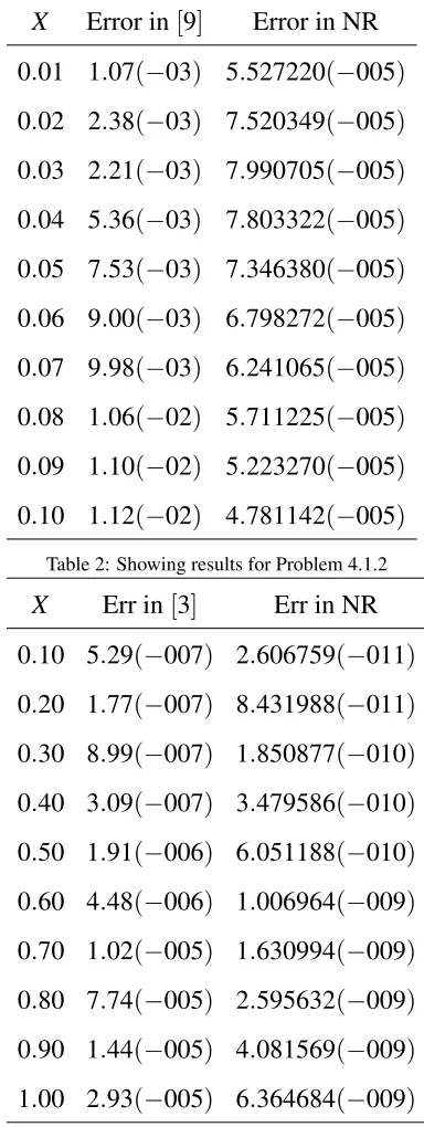
Table 1 Showing results for Problem 4.1.1
X Error in[9] Error in NR 0.01 1.07(−03) 5.527220(−005) 0.02 2.38(−03) 7.520349(−005) 0.03 2.21(−03) 7.990705(−005) 0.04 5.36(−03) 7.803322(−005) 0.05 7.53(−03) 7.346380(−005) 0.06 9.00(−03) 6.798272(−005) 0.07 9.98(−03) 6.241065(−005) 0.08 1.06(−02) 5.711225(−005) 0.09 1.10(−02) 5.223270(−005) 0.10 1.12(−02) 4.781142(−005)
Table 2: Showing results for Problem 4.1.2
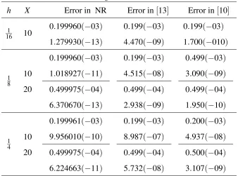
Table 3:Showing results for Problem 4.1.3
h X Error in NR Error in[13] Error in[10]
1
16 10
0.199960(−03) 1.279930(−13)
0.199(−03) 4.470(−09)
0.199(−03) 1.700(−010)
1 8
10 20
0.199960(−03) 1.018927(−11) 0.499975(−04) 6.370670(−13)
0.199(−03) 4.515(−08) 0.499(−04) 2.938(−09)
0.499(−03) 3.090(−09) 0.499(−04) 1.950(−10)
1 4
10 20
0.199961(−03) 9.956010(−10) 0.499975(−04) 6.224663(−11)
0.199(−03) 8.987(−07) 0.499(−04) 5.732(−08)
0.200(−03) 4.937(−08) 0.500(−04) 3.107(−09)
4.2. Discussion of result
Problem 4.1.1 was solved by [9] where a three block backward differenciation formula was proposed. Problem 4.1.2 was solved by [3] where a stiff starting block method of order six was proposed. Problem 4.1.3 was solved by [10]. Table 1-3 shows clearly that our method performed better in term of accuracy than the existing method.The method proposed by [13] and [10] are of order six and four respectively.
5. Conclusion
We have proposed a non self starting continuous block method in this paper. The continuous block method enable us to evaluate a given problem at all the points within the interval of inte-gration without starting the block all over.This property enables us to understand the behaviour of a dynamical system at any given point within the interval of integration. It had been shown from the examples given that the non self starting method gives better approximation than the self starting method.
Conflict of Interests
REFERENCES
[1] A.O. Adesanya, M.O. Udoh, A.M. Ajileye, A new hybrid block method for the solution of general third order initial value problems of ordinary differential equations, Int. J. Pure Appl. Math. 86 (2013), 365-375. [2] A.O. Adesanya, M.R. Odekunle, M.O. Udoh, FOur steps continuous method for the solution of y00 =
f(x,y.y0),Amer. J. Comput. Math. 3 (2013), 169-174.
[3] A.A. James, A.O. Adesanya, S. Joshua, Continuous block method for the solution of second order initial value problems of ordinary differential equations, Int. J. pure Appl. Math. 88 (2013), 405-416.
[4] A.M. Badmus, D.W. Mishelia, Some uniform order block method for the solution of first-order differential equations, J. Nigeria Assoc. Math. phys. 19 (2011), 149-154.
[5] S.O. Fatunla, Numerical methods for Initial Value Problems in Ordinary Differential Equations, New-York, Academic Press 1988.
[6] P.W. Gaffery, A performance evaluation of some FORTRAN subroutine for the solution of stiff oscillatory ODE’s, ACM Trans. Math. software 10 (1984), 58-72.
[7] J. Sunday, M.R. Odekunle, A.O. Adesanya, Order six block integrator for the solution of first-order differen-tial equations, Int. J. Math. Soft Comput. 3 (2012), 87-96.
[8] J.D. Lambert, Computational Methods in Ordinary Differential Equations. John Wiley, New York, 1973. [9] S.A. Okunuga, A.B. Sofoluwe, J.O. Ehigie, Some block numerical schemes for solving initial value problems
in ODEs, J. Math. Sci. 2 (2013), 387-402.
[10] R.K. Jain, Some A-Stable methods for stiff ordinary differential equations, Math. Comput. 26 (1972), 71-77. [11] S.N. Jator, A six order linear multistep method for direct solution ofy00=f(x,y.y0),Int. J. Pure appl. Math. 4
(2007), 457-472.
[12] S.N. Jator, On a class of hybrid method fory00=f(x,y.y0),Int. J. Pure Appl. Math. 59 (2010), 381-395. [13] S.P. Norsett. An a-stable modification of the Adams-Bashforth methods. In: Conference on the Numerical
Solution of Differential Equations. Dundee, Scotland (1969).
[14] T.A. Anake, D.O. Awoyemi, A.O. Adesanya, One step implicit hybrid block method for the direct solution of general second order ordinary differential equations, IAENG Int. J. Appl. Math. (2012).