Annually, around 50 million people get injured in automobile accidents and around 1.25 million die around the world [48]. Most of these casualties are due to preventable driver-borne causes like distracted driving, reckless driving, speeding, disobeying traffic signs, etc. Autonomous driving, let it be fully autonomous or assistive, can significantly reduce such human errors and hence reducing number of traffic accidents. In addition, such technology also reduces human effort, stress, and leads to better traffic management.
by
Harsh Virendra Pandya
A thesis submitted to the Graduate Faculty of North Carolina State University
in partial fulfillment of the requirements for the degree of
Master of Science
Electrical Engineering
Raleigh, North Carolina 2015
APPROVED BY:
_______________________________ _______________________________
Dr. Wesley Snyder Dr. Edward Grant
_______________________________ Dr. Edgar Lobaton
BIOGRAPHY
Harsh Pandya was born in the year 1991 in Vadodara, India. He completed his undergraduate degree (Bachelor of Engineering in Electronics) from The Maharaja Sayajirao University of Baroda in 2012.
ACKNOWLEDGMENTS
I would like to thank Dr. Edgar Lobaton, my advisor, for his guidance and support throughout my thesis research. Starting from the inception of this idea, nailing down the milestones to finishing up the writing, he has played a significant role in the advancement of my research.
Special thanks to Dr. Wesley Snyder for inspiring me to further my research. If it were not for you, I might have never embraced Computer Vision so much. I would also like to thank Dr. Edward Grant for teaching me the very bare bone essentials of robotics viz. Kinematics and Dynamics. I cannot imagine my research without the knowledge that I gained from both of you.
A special thanks to Jeremy Cole for clearing my doubts and helping me with hardware issues; thanks to Qian for her contribution to the implementation of RANSAC in MATLAB. I also thank Sahil, Somrita, Alireza, Daniel, and Namita for their cooperation in the lab.
TABLE OF CONTENTS
List of Figures ………...………... vii
Chapter 1 Introduction ………. 1
1.1 Motivation and problem overview ………... 1
1.2 System Overview and Contribution ………..………...… 5
1.3 Thesis Organization ……… 7
Chapter 2 Hardware Platform ………...…. 8
2.1 Husky Unmanned Ground Vehicle ………... 10
2.2 Kinova Jaco Robotic Arm ………... 13
2.3 Microsoft Kinect ………..……….... 15
2.4 Asus Eee 1215N Netbook ………...………… 17
Chapter 3 Software Platform ………..………. 19
3.1 Virtual Robot Experimentation Platform (V-REP) ………....….. 19
3.1.1 Scene creation and model setup ………... 22
3.1.2 Calculation Modules ………..…. 25
3.2 Robot Operating System (ROS) ………..…. 27
3.2.1 jaco_ros package ………... 31
3.2.2 openni_camera package ………..……….... 33
3.2.3 husky_base package ………..…. 36
3.2.4 image_acquisition package ………...………... 37
Chapter 4 Motion Planning and Image Acquisition ………..….. 38
4.1 V-REP ……….. 39
4.1.1 Kinematic Simulations ……….. 41
4.1.2 Precise Object Tracking ………..………. 48
4.1.3 Final Framework Simulation ………..…….. 51
4.2 ROS Framework ………... 54
Chapter 5 Ground Segmentation ………..……. 57
5.1 RANSAC for Plane fitting ………..……... 59
5.2 Ground Segmentation using RANSAC ………..…... 60
Chapter 6 Kinect View Validation Framework (KVVF) …...………. 63
6.2 Low Level Operation ……….. 68
Chapter 7 Results ………..………...………..…... 70
7.1 Experimental Setup ……….... 70
7.2 Evaluation ………... 73
Chapter 8 Conclusion and Future Work………...……….... 79
LIST OF FIGURES
Figure 1.1 System Overview ………. 5
Figure 2.1 Hardware Platform ……….... 9
Figure 2.2 Husky A200 Isometric view and reference frame ………... 10
Figure 2.3 Husky A200 front and rear with component labels ………... 11
Figure 2.4 Jaco Arm with various parts labelled ……….. 13
Figure 2.5 Jaco Arm base with connectors ………..…….... 14
Figure 2.6 Microsoft Kinect ………... 15
Figure 2.7 Asus Eee 1215N ……….... 17
Figure 3.1 Control architecture in V-REP. Greyed areas are user customizable …….. 21
Figure 3.2 Scene hierarchy in V-REP ………... 22
Figure 3.3 Top: V-REP main screen; Bottom: A scene in V-REP with various Components …..……….… 23
Figure 3.4 Simulation Loop in V-REP ……….. 26
Figure 3.5 Communication in ROS among nodes ……….… 29
Figure 3.6 Role of Master in ROS communication ………... 30
Figure 3.7 image_view RGB ………... 34
Figure 3.8 image_view Depth ………... 34
Figure 3.9 image_view Disparity ……… 35
Figure 4.1 Two kinematic chains, each describing an IK element ……… 42
Figure 4.2 IK element and corresponding model of the IK solving task ……… 43
Figure 4.3 IK chain and constraints ……….…. 44
Figure 4.4 IK task menu and options ………... 45
Figure 4.5 Jaco workspace ……….… 46
Figure 4.6 IK chain in Jaco arm ………... 47
Figure 4.7 Euler angles ……….… 49
Figure 4.8 Object tracking using Jaco arm ……….... 50
Figure 4.9 Final platform simulation ………...………... 52
Figure 4.10 Jaco single time frame configurations ………. 53
Figure 4.11 Software framework workflow ………... 55
Figure 5.2 Ground Plane Detection Using RANSAC [27] ……….……. 59
Figure 5.3 Left: Disparity map; Right: Ground pixels used for fitting ……….…. 61
Figure 5.4 Top: Ground plane obtained by RANSAC; Bottom Left: Ground segmentation using plane fitting; Bottom Right: Obstacle segmentation/separation ……….…… 62
Figure 6.1 Kinect View front end; 1: Frame/path selection; 2: Path display; 3: image view window; 4: options………... 64
Figure 6.2 Kinect View front end; 1: Frame/path selection; 2: Path display; With Path Selection mode ON ……….…. 66
Figure 6.3 Kinect View front end; 3: image view window; 4: options with Single View mode On ……….. 67
Figure 7.1 Kinect motion trajectory ……….…… 71
Figure 7.2 Recorded data at different time frames …...……….……. 72
Figure 7.3 Selection of candidate pixels for ground plane……….…. 73
Figure 7.4 Random trajectory data stream (Trajectory from Figure 6.2)...…..………… 75
Figure 7.5 Five random trajectories…...……….. 76
Figure 7.6 Red: Mean trajectory; Blue: (Mean-stdv) trajectory; Yellow: (Mean+stdv) trajectory……….……….… 77
Figure 7.7 Overlap ratio for individual trajectories………..……….…. 78
Chapter 1
Introduction
1.1 Motivation and problem overview
Traffic accidents retain to be a major source of disability and mortality worldwide. Every year, 1.25 million people die and up to 50 million people are injured [48, 45]. Autonomous or driver-assistive cars have the potential to reduce these numbers dramatically by the virtue of reducing human errors. Apart from accidental concerns, Urbanization is such a substantial demographic trend [41] that affects millions of people worldwide, which is particularly observable for numerous growing megacities [28]. This results in chronic track congestion, air pollution, slow speed in rush hours, and the struggle for finding empty parking spots, which has become overly annoying [47]. This has also lead general public, a majority of which includes commuters, to increasingly demand alternatives for their personal mobility, culminating in about one third of drivers being interested in buying an affordable self-driving car [5, 47]. A substantial aspect of tomorrows urban mobility is most likely going to be personal self-driving cars and autonomous car fleets that provide solutions for these challenges [35].
improved [25]. Moreover, the maturity of this technology has reached a level enough to enable a fully autonomous vehicle to drive complying with urban traffic laws [10].
[21, 25] demonstrate that autonomous vehicles can be successful in challenging environments. The DARPA Grand and Urban Challenge competitions (2005, 2007) [23, 11] offer a modern, uniform testing opportunity to examine the state-of-the-art in autonomous cars.
As mentioned before, work on self-driving cars spans several decades [15, 37, 22, 9]. Especially in the past decade considerable amount of work has been done in the area of autonomous driving. The basic idea revolves around using a sensor suite for collecting data about the surroundings of the car and then classifying/tracking/detecting various elements in the environment. The said sensor suite ranges from expensive LiDAR systems to inexpensive stereo camera systems based on the level of autonomy and accuracy demonstrated by the overall system. For good and sufficient sensing information, there are two primary approaches: long range and wide angle sensor equipment, and distributed perception [32, 40]. The high performance sensors provide an immediate response sensing time or large area sensing capability, but whose price is prohibitively expensive for economic viability, and sensing area is limited by line-of-sight [24].
A dataset consisting of multiple perspective data streams serves two major purposes when used for algorithmic testing:
1. Evaluating the sensitivity of an algorithm/technique to trajectory perturbations/disturbances. It is quite common for vehicles to not follow a smooth trajectory on the roads due to several factors like unfavorable weather conditions, ill-conditioned roads, spills, obstacles, other vehicles, change in overall traffic speed, etc. It is such situations that, to some extent, contribute to human errors, resulting into an accident. The same can be applied to autonomous vehicles; when they experience a perturbation in the trajectory of their motion, the data streams captured by their sensor suite lose continuity. This might lead to the failure of one or more algorithms (e.g. obstacle tracking failure as an obstacle fled the field of view of the camera). A dataset with multiple perspectives can be used to simulate such perturbations and test any given algorithm/technique to find out whether it fails in such situations.
Techniques/algorithms for such system can be easily tested using our multi-perspective dataset.
In order to generate our dataset, we use a Mobile Manipulator equipped with a 6 DOF arm for manipulating the position and orientation of a Microsoft Kinect for capturing depth images from multiple perspectives. ROS (Robot Operating System) forms the backbone of our software framework providing necessary communication between various hardware components. Further the registered depth and brightness images captured are processed using Kinect View – a Matlab based GUI program for data extraction, path selection, and testing techniques used in autonomous driving. Kinect View is capable of creating random trajectories on the plane and generating datastreams by selecting specific views from the dataset of depth images.
1.2 System Overview and Contribution
The block diagram below provides a bird’s eye view of our framework and the dataflow within it:
Figure 1.1: System Overview
performs analysis and tests algorithmic performance. Original work done during the course of this thesis includes:
V-REP development: Created various simulation experiments on V-REP, wrote scripts for individual objects in the scenes, motion planning, and data extraction.
Created Image_acquisition package in ROS to facilitate the communication between hardware driver packages like openni_camera, husky_base, and jaco_ros.
New nodes to facilitate image capturing using openni.
Kinect camera calibration.
MATLAB based GUI for Kinect View.
Backend scripts to control the Kinect View behavior dynamically.
Random path generation using biased graph walk with data stream extraction.
RANSAC plane fitting for ground segmentation.
1.3 Thesis Organization
Chapter 1 introduced the autonomous driving problem, general approach to resolve it, and our platform for data collection and testing various techniques. Upcoming chapters are organized as follows:
Chapter 2 describes the hardware platform used in our framework. It describes the basic properties and features expected from the hardware platform, introduces individual elements in the system, and fleshes out how they fit the role.
Chapter 3 introduces the software platforms used for our framework. It goes into explaining the GUI based simulation software V-REP used for scene setup and motion planning. It also introduces ROS, the backbone of our framework, and various packages used for interacting with individual hardware components.
Chapter 4 goes into motion planning and data collection with several experimental setups. Moreover, it also details out the flow of data, and the underlying pipeline of operation, how individual pieces interact with each other and how final dataset is acquired.
Chapter 5 introduces ground segmentation as a means of exploring the proof of concept for the said framework. We use a RANSAC based plane fitting approach for ground plane fitting and eventual segmentation.
Chapter 6 discusses the MATLAB based GUI program called Kinect_View, developed for analyzing the data captured using our framework. This chapter explains the program architecture and various functionalities in detail. Kinect_View is highly modular, in that one can plug in any image processing algorithm/technique for testing and analysis.
Chapter 2
Hardware Platform
This Chapter describes the Hardware Platform created for the said framework. The platform was created with following qualities in mind:
Mobility – The platform needs to emulate a vehicle to certain extent in order to collect data sets for testing autonomous driving techniques. Hence it should be fairly mobile.
Agility – The platform has to be agile with precise movement control as the orientation and position of camera while recording frames has to be accurate. High level of controllability is desirable.
Ease-of-interface – Each individual component of the hardware platform should be able to communicate with other components directly or indirectly using some common platform.
Remote and local control – Finally, It is desirable to have an onboard computing unit on the platform for local control and analysis. It should also be possible to control and collect data remotely.
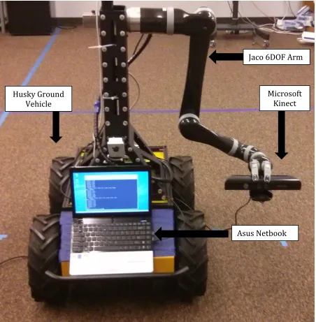
Figure 2.1: Hardware Platform
Jaco 6DOF Arm
Asus Netbook Husky Ground
Vehicle
2.1 Husky Unmanned Ground Vehicle
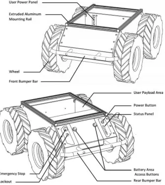
Husky A200 robot from Clearpath Robotics is a rugged and easy-to-use unmanned ground vehicle for rapid prototyping and research applications. Figure 2.2 provides an isometric view of Husky. The robot is extremely basic, in that it comes with only the base: wheels, motors, chassis, battery, and a simple lockdown mechanism. Yet its rugged nature, payload capacity and agility make it a perfect base for our manipulator platform.
Figure 2.2: Husky A200 Isometric view and reference frame
We follow a Cartesian reference frame based on ISO 8855 for non-holonomic motion, and is shown in Figure 2.2. In terms of dimension it is 990mm long, 670mm wide and 390mm high. The Husky A200 weighs about 50kg and has a payload capacity of 75kg. It can go up to 1m/s maximum speed and climb up to 45°.
Figure 2.3: Husky A200 front and rear with component labels
The relationship between wheel velocity and platform velocity is governed by:
𝑣 =
𝑣𝑙+𝑣𝑟2
,
ω =
𝑣𝑟−𝑣𝑙𝑤
where 𝑣 represents the instantaneous translational speed of the platform and ω the
instantaneous rotational speed. 𝑣𝑟 and 𝑣𝑙 are the right and left wheel velocities,
Husky supports four distinct control modes:
Kinematic Control, the default, uses a speed control feedback loop, and allows specifying the desired linear and angular speed of Husky.
Torque Control, the linear and angular values specified are multiplied by parameterized scaling factors and used for a current control feedback loop.
2.2 Kinova Jaco Robotic Arm
The JACO arm is a light-weight, technical assistance robot designed to mimic mobility of the upper limbs. It is composed of six inter-linked segments, the last of which is a three-fingered hand. The robot’s hand is capable of movement in three dimensional space and grasp or release objects with the hand. The JACO arm has a weight of 5.6kg, can reach approximately 90cm in all directions and can lift objects of up to 1.5kg.
The six joints of the JACO, as shown in Figure 2.4, are individually driven by six DC geared servomotors located in each joint. Each motor module includes a planetary gearhead. Two types of motor modules are used depending on joint location in the kinematic chain. Joints 1–3, where joint 1 the nearest to the base, use large motor modules while joints 4–6 use small motor modules [13].
Within a single manipulator, each motor module is interchangeable in terms of its position based on its class. That is to say, a small motor module can replace any motor module of joints 4–6 without any effect on the performance of the arm. The carbon-fiber links house the series of motor modules at the links while wiring is routed through the hollow members. Each finger in the end effector is driven by an individual motor bringing the sum of motors to 9 [13].
Figure 2.5: Jaco Arm base with connectors
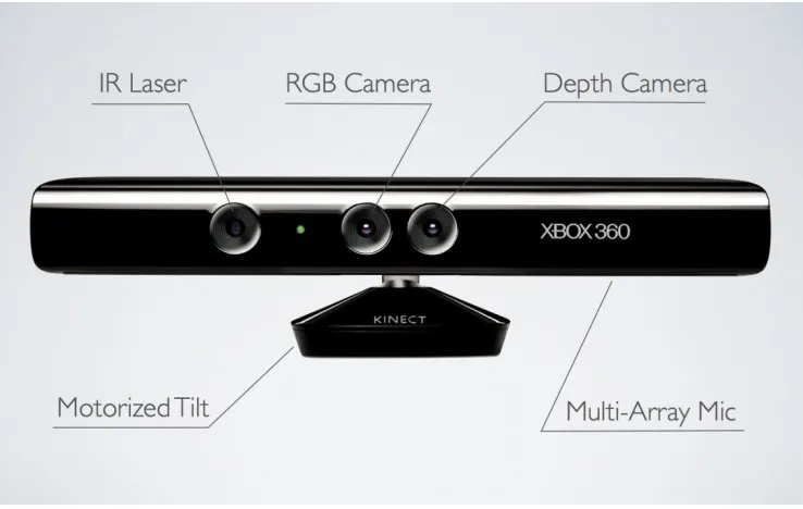
2.3 Microsoft Kinect
Originally intended to be used as an input device for Microsoft’s Xbox 360 gaming console, the Kinect (Figure 2.6) contains a diverse set of sensors. Most notable of those sensors being a depth camera based on infrared structured light technology [44]. With a proper calibration of its color and depth cameras, the Kinect can capture detailed color point clouds at up to 30 frames per second. This capability uniquely positions the Kinect for use in fields other than entertainment, such as robotics, natural user interfaces, and three-dimensional mapping.
Figure 2.6: Microsoft Kinect
camera system consists of paired CMOS infrared and color cameras and an infrared structured light projector. Both cameras sit in the Kinect’s middle on either side of its standoff whereas the structured light projector is displaced towards the Kinect’s left side (as viewed from the front). Using stereo calibration, the cameras are measured as roughly 2.5cm apart, and a similar method measures the separation between the structured light projector and infrared camera as roughly 7.5cm [12, 26].
Microsoft’s official Kinect programming guide specifies the system’s field of view as 43° vertical by 57° horizontal, the color and depth image sizes as VGA and QVGA respectively, the “playable range” as 1.2m to 3.5m, and the frame rate as 30Hz [33]. Based upon the PrimeSensor Reference Design specifications, the Kinect’s expected depth resolution at 2m is 1cm [38]. The Kinect’s infrared structured light projector emits the pattern resembles the illumination scheme described by [18], one of PrimeSense’s depth imaging patents. According to the patent, the pattern consists of pseudo-random spots such that any particular local collection of spots (a “speckle feature”) is uncorrelated with the remainder of the pattern [16]. Thus, a known speckle feature is uniquely identifiable and locatable in an image of the structured light pattern. In addition to the color and depth camera system, the Kinect includes an array of four microphones, a three-axis accelerometer, and a tilt motor. The microphone array is capable of beamforming, source localization, and speech recognition with the assistance of a host computer, although the Kinect can perform on-board echo cancellation and noise suppression [33, 16]. The tilt motor can angle the Kinect ±31° from horizontal and works in conjunction with the accelerometer to level the Kinect on an angled surface [36].
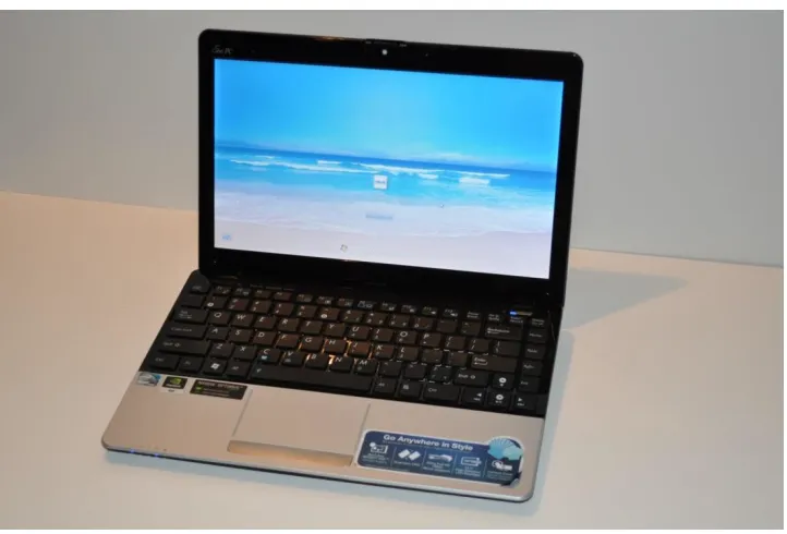
2.4 Asus Eee 1215N Netbook
As a local computing unit for our hardware platform, we use a lightweight Asus 1215N netbook. The Asus 1215N netbook runs on a 1.8GHz Intel® Atom™ D525 (Dual Core) Processor. It has 1GB DDR1 RAM with 250GB SATA hard drive. Wireless connectivity in the form of WLAN 802.11 a/b/g/n and Bluetooth V3.0+HS is available. It also provides various interface options like 1 x VGA Connector, 1 x USB 2.0, 2 x USB 3.0, 1 x LAN RJ-45, and 1 x HDMI.
Figure 2.7: Asus Eee 1215N
All the preinstalled software packages, including the Operating System, were removed and a fresh Ubuntu 12.04.5 LTS (Precise Pangolin) was installed. To support the said framework development, following software packages were installed:
ROS Hydro Medusa (Robot Operating System 7)
V-REP 3.2.0 (Virtual Robot Experimentation Platform)
OpenCV 2.4.4
Chapter 3
Software Platform
As mentioned in previous chapter, ease-of-interface among various components was one of the basic requirements for this platform. We chose Robot Operating System (ROS) Hydro as the backbone for our software framework, while Virtual Robot Experimentation Platform (V-REP) was used extensively for simulations and motion planning.
3.1 Virtual Robot Experimentation Platform (V-REP)
V-REP is like a Swiss army knife among robot simulator platforms, it is equipped with a plethora of functions, features, and elaborate APIs. V-REP PRO EDU license is free to use, fully functional simulation platform available to use for non-commercial, educational, and research purposes.
Following are a few of V-REP's applications:
Simulation of factory automation systems
Remote monitoring
Hardware control
Fast prototyping and verification
Safety monitoring
Fast algorithm development
Robotics related education
Product presentation
V-REP can be used as a stand-alone application or can easily be embedded into a main client application: its small footprint and elaborate API makes V-REP an ideal candidate to embed into higher-level applications. An integrated Lua script interpreter makes V-REP an extremely versatile application, leaving the freedom to the user to combine the low/high-level functionalities to obtain new high-level functionalities.
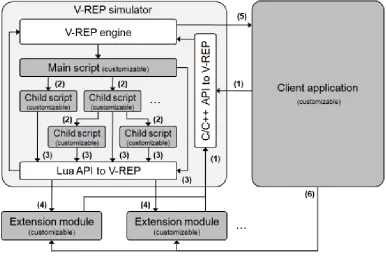
Figure 3.1: Control architecture in V-REP. Greyed areas are user customizable
In addition, custom simulation functions can be added via:
Scripts in the Lua language. Lua [1] is a lightweight extension programming language designed to support procedural programming. The Lua script interpreter is embedded in V-REP, and extended with several hundreds of VREP specific commands. Scripts in V-REP are the main control mechanism for a simulation.
3.1.1
Scene creation and model setup
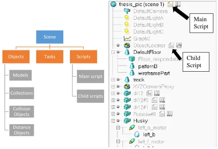
Each new simulation in V-REP begins with a scene. Simulations in V-REP are hierarchical where a Scene can be considered as the root of the hierarchy. This scene in turn may contain various objects, models, tasks, and scripts. Figure 3.2 shows the structure and components of a typical scene in V-REP.
Figure 3.2: Scene hierarchy in V-REP Scene
Objects
Models
Collections
Collision Objects
Distance Objects
Tasks Scripts
Main script
Child scripts
Main Script
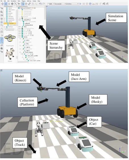
Figure 3.3: Top: V-REP main screen; Bottom: A scene in V-REP with various components Simulation Scene
Scene hierarchy
Model (Husky)
Object (Car) Model
(Kinect)
Model (Jaco Arm)
One of the scenes created for the framework is shown in figure 3.3. This scene consists of several objects, collections, scripts, and models. Some of the models were readily available for use (e.g. Jaco Arm), while others were custom created from basic shapes, assigning physical properties like density, material type, center of mass, etc. (e.g. Husky robot and tower assembly). Models or objects can be dragged and dropped from Model browser. The scene can be rotated, tilted, or dragged using camera navigation toolbar. Individual objects can be accessed by single clicking in either the scene or the hierarchy. Object manipulation tool can be used to rotate or translate selected object in 3D space.
A simulation is handled when the client application calls a main script, which in turn can call child scripts. Each simulation scene has exactly one main script that handles all default behaviour of a simulation, allowing simple simulations to run without even writing a single line of code. The main script is called at every simulation pass and is non-threaded.
Child scripts on the other hand are not limited in number, and are associated with (or attached to) scene objects. As such, they are automatically duplicated if the associated scene object is duplicated. In addition to that, duplicated scripts do not need any code adjustment and will automatically fetch correct object handles when accessing them. Child scripts can be non-threaded or threaded (i.e. launch a new thread).
3.1.2
Calculation Modules
Scene objects are rarely used on their own, they rather operate on (or in conjunction with) other scene objects (e.g. a proximity sensor will detect shapes or dummies that intersect with its detection volume). In addition, V-REP has several calculation modules that can directly operate on one or several scene objects. Following are V-REP’s main calculation modules [19]:
Forward and inverse kinematics module: allows kinematics calculations for any type of mechanism (branched, closed, redundant, containing nested loops, etc.). The module is based on calculation of the damped least squares pseudoinverse [46]. It supports conditional solving, damped and weighted resolution, and obstacle avoidance based contraints.
Dynamics or physics module: allows handling rigid body dynamics calculation and interaction (collision response, grasping, etc.) via the Bullet Physics Library [2].
Path planning module: allows holonomic path planning tasks and non-holonomic path planning tasks (for car-like vehicles) via an approach derived from the Rapidly-exploring Random Tree (RRT) algorithm [30].
Collision detection module: allows fast interference checking between any shape or collection of shapes. Optionally, the collision contour can also be calculated. The module uses data structures based on a binary tree of Oriented Bounding Boxes [20] for accelerations. Additional optimization is achieved with a temporal coherency caching technique.
Except for the dynamics or physics modules that directly operate on all dynamically enabled scene objects, other calculation modules require the definition of a calculation task or calculation object, that specifies on which scene objects the module should operate and how. If for example the user wishes to have the minimum distance between shape A and shape B automatically calculated and maybe also recorded, then a minimum distance object has to be defined, having as parameters shape A and shape B. Figure 3.4 shows V-REP’s typical simulation loop, including main scene objects and calculation modules.
3.2 Robot Operating System (ROS)
In spite of rapid progress in the field of robotics in the past few decades, robots still present significant challenges for software developers. From the robot's perspective, problems that seem trivial to humans often vary wildly between instances of tasks and environments. Often robotic systems, tackling real life problems, require complex integration of sensor suites, one or more robotic platforms, and various actuators. A common framework/platform built upon features like:
Solid communication Infrastructure
Robot-Specific features
Elimination of programming language barrier
Diagnostic tools
Advance Simulation capabilities
can eliminate most, if not all, aforementioned challenges in robotic software development.
With a mission of creating truly robust, general-purpose robot software, Willow Garage came up with a software platform called Robot Operating System, or ROS that is intended to ease some of these difficulties. The official description of ROS is:
“ROS is an open-source, meta-operating system for your robot. It provides the services you would expect from an operating system, including hardware abstraction, low-level device control, implementation of commonly-used functionality, message-passing between processes, and package management. It also provides tools and libraries for obtaining, building, writing, and running code across multiple computers.”
Before we describe the communication protocol and how data passes along various aspects of ROS, here are a few key concepts one must know [14]:
Packages: Packages are the main unit for organizing software in ROS. A package may contain ROS runtime processes (nodes), a ROS-dependent library, datasets, configuration files, or anything else that is usefully organized together. Packages are the most atomic build item and release item in ROS.
Nodes: Nodes are process that can perform computation, execute some tasks and communicate thanks to the ROS network. Each node registers to the network with a unique id and a list of topics and services that it wants to send or receive messages from and some additional connection parameters. ROS provides libraries to write the nodes with the C++ or the Python languages.
Master: The master is a special node that is launched every time ROS is started. It handles the registration, subscriptions and disconnection of every node to the network and links for each topic or service so that messages will be able to reach its target successfully. The ROS Master provides name registration and lookup to the rest of the Computation Graph. Without the Master, nodes would not be able to find each other, exchange messages, or invoke services.
Messages: Packets sent on the network are defined in ROS messages. Nodes communicate with each other by passing messages. A message is simply a data structure, comprising typed fields. Standard primitive types (integer, floating point, boolean, etc.) are supported, as are arrays of primitive types. Messages can include arbitrarily nested structures and arrays (much like C structs).
general, publishers and subscribers are not aware of each other’s existence. The idea is to decouple the production of information from its consumption. Logically, one can think of a topic as a strongly typed message bus. Each bus has a name, and anyone can connect to the bus to send or receive messages as long as they are the right type.
Services: The publish/subscribe model is a very flexible communication paradigm, but its many-to-many, one-way transport is not appropriate for request/reply interactions, which are often required in a distributed system. Request/reply is done via services (Figure 3.5), which are defined by a pair of message structures: one for the request and one for the reply. A providing node offers a service under a name and a client uses the service by sending the request message and awaiting the reply. ROS client libraries generally present this interaction to the programmer as if it were a remote procedure call.
Figure 3.5: Communication in ROS among nodes
Topic
Node
Node
Node
Service
Node
Node
Node
[14] The ROS Master acts as a nameservice in the ROS Computation Graph. It stores topics and services registration information for ROS nodes. Nodes communicate with the Master to report their registration information. As these nodes communicate with the Master, they can receive information about other registered nodes and make connections as appropriate (Figure 3.6). The Master will also make callbacks to these nodes when the registration information changes. This allows nodes to dynamically create connections as new nodes are run.
Figure 3.6: Role of Master in ROS communication
This architecture allows for decoupled operation, where the names are the primary means by which larger and more complex systems can be built. Names have a very important role in ROS: nodes, topics, services, and parameters all have names. Every ROS client library supports command-line remapping of names, which means a compiled program can be reconfigured at runtime to operate in a different Computation Graph topology.
The rest of this chapter focusses on individual ROS packages used to control individual hardware components of our platform. These packages are described in details pertaining to various nodes, topics, and services they offer.
3.2.1
jaco_ros package
The ROS JACO Arm metapackage provides a ROS interface for the Kinova Robotics JACO robotic manipulator arm. This metapackage provides access to the Kinova JACO C++ hardware API through ROS.
The JACO API is exposed to ROS using a combination of actionlib (for sending trajectory commands to the arm), services (for instant control such as homing the arm or e-stop) and published topics (joint feedback). The arm may be commanded using either angular commands or cartesian co-ordinates. In addition, a transform publisher enables visualization of the arm via rviz.
There are three actionlib modules available: arm_pose/arm_pose, joint_angles/arm_joint_angles, and fingers/finger_position. These server modules accept coordinates which are passed on to the Kinova JACO API for controlling the arm.
Published topics are: out/cartesian_velocity, out/joint_velocity, out/finger_position, out/joint_angles, out/joint_state, and out/tool_position. The cartesian_velocity and joint_velocity are both subscribers which may be used to set the joint velocity of the arm. The finger_position and joint_angles topics publish the raw angular position of the fingers and joints, respectively, in degrees. The joint_state topic publishes via sensor_msgs the transformed joint angles in radians. The tool_position topic publishes the Cartesian co-ordinates of the arm and end effector via geometry_msgs.
The jaco_arm_driver node acts as an interface between the Kinova JACO C++ API and the various actionservers, message services and topics used to interface with the arm. The jaco_tf_updater node subscribes to the jaco_arm_driver node to obtain current joint angle information from the node. It then publishes a transform which may be used in visualization programs such as rviz.
In our case none of the inverse kinematic topic subscribers seemed to work, hence we decided to use V-REP as our inverse kinematics and motion planning tool. Details about message structure and parameters for each of the above mentioned topics and services can be found at [7]. Some of the basic services and topics used most frequently are:
To “home” the arm
rosservice call /jaco_arm_driver/in/home_arm
To activate the emergency stop function
rosservice call /jaco_arm_driver/in/stop
To restore control of the arm
rosservice call /jaco_arm_driver/in/start
To obtain the raw joint angles in degrees
rostopic echo jaco/joint_angles
To obtain the finger angles in degrees
To obtain the arm’s position in Cartesian units
rostopic echo jaco/tool_position
3.2.2
openni_camera package
A ROS package that contains OpenNI driver for RGB+D cameras that includes Microsoft Kinect, PrimeSense PSDK, ASUS Xtion Pro and Pro Live. This package publishes raw depth, RGB, and IR image streams using the ROS message-passing system. OpenNI, in itself, is the largest 3-D sensing development framework and community that provides an open source SDK.
There are two formats of the depth channel output — disparity map or the real depth in millimetres. The sensor returns the disparity value and the driver is by default configured to convert this value to the real depth. The disparity of the pixel represents the shift of a point in two stereoscopic images [39] (analogically for the pattern projected by the IR projector and captured by the IR camera). In the PrimeSense terminology, the disparity is called a shift value.
This package also contains launch files for using OpenNI-compliant devices such as the Microsoft Kinect in ROS. It creates a nodelet graph to transform raw data from the device driver into point clouds, disparity images, and other products suitable for processing and visualization. Openni_launch launches in one process the device driver and many processing nodelets for turning the raw RGB and depth images into useful products, such as point clouds. Provides default tf tree linking the RGB and depth cameras [4].
RGB image:
rosrun image_view image_view image:=/camera/rgb/image_color
Figure 3.7: image_view RGB
Depth image:
rosrun image_view image_view image:=/camera/depth/image
image_view also contains the disparity_view viewer for sensor_msgs/DisparityImage messages:
rosrun image_view disparity_view image:=/camera/depth/disparity
Figure 3.9: image_view Disparity
Topics published by openni_camera are:
camera/depth/image_raw (sensor_msgs/Image) uint16 depth image in mm, the native OpenNI format.
camera/rgb/image_raw (sensor_msgs/Image)
Raw image stream from the camera driver, the native OpenNI format.
camera/rgb/camera_info (sensor_msgs/CameraInfo) Camera calibration and metadata.
These topics are then used by support packages like image_proc and depth_image_proc which publish new topics with registered images, rectified images, converting data type of encoded data streams, creating a point cloud stream for visualization in rviz, etc.
3.2.3
husky_base package
This ROS package contains Clearpath’s driver for husky. The husky_base package contains a node for communicating with the Husky MCU, and launch files to bring up the Husky control and diagnostic systems. The husky_node hardware interface is configured through the husky_control package.
It is subscribed to a single topic:
husky_velocity_controller/cmd_vel (geometry_msgs/Twist)
Twist velocity command for Husky MCU, muxed in husky_control. External clients should publish to bare cmd_vel topic.
While it publishes a couple of topics:
husky_velocity_controller/odom (nav_msgs/Odometry) Odometry information from Husky MCU.
status (husky_msgs/HuskyStatus)
Status information from Husky MCU and husky_node. Also exposed over standard diagnostics interface.
3.2.4
image_acquisition package
We created this ROS package to establish flow of data between V-REP and other ROS packages. It contains two nodes:
messenger_node: Communication bridge between V-REP and ROS. Converts motion planning data obtained from V-REP into a custom message format for other nodes to work with.
reader_node: Manages activation and suspension of multiple nodes in oppeni_camera, jaco_ros, and husky_base. It basically controls the activation of those nodes by waiting for specific events to occur like arm reaching desired configuration or Kinect finishing up saving images.
Chapter 4
Motion Planning and Image Acquisition
In order to generate a desirable image set, precise positioning of the camera is of utmost importance. Not only positioning but its traversal through the 3D workspace has to be compliant, collision free, and optimal (in terms of uniformity of motion). The hardware platform described in chapter 3 was initially simulated in a physics engine based simulator called Virtual Robot Experimentation Platform (V-REP), before actual implementation.
4.1 V-REP
As shown in section 3.1, V-REP is capable of replicating/simulating the entire setup for our platform. We sample the angular positions for each joint in Jaco Arm, as well as the motors in Husky robot wheels, based on simulation time. This provides us a profile of joint space configurations for the Jaco arm to transition through forward kinematically and achieve the required trajectory for capturing the data set.
But before using the raw position values for Jaco joints, they have to be processed in order to account for the differences between physical joints and simulated joints. The physical joint motors are limted to a range of -180 to +180, while there is no such limitation on the simulated joints, hence a simple conversion needs to take place before the joint positions can be used. For the Right Jaco arm, following conversions were performed:
Joint 1: P_ang= - (S_ang+90)
Joint 2: P_ang= S_ang+90
Joint 3: P_ang= - (S_ang-90)
Joint 4: P_ang= - (S_ang-180)
Joint 5: P_ang= - (S_ang-180)
Joint 6: P_ang= - (S_ang+270)
The child script attached to the Jaco Arm performs the aforementioned conversion before publishing the joint configurations. The conversion takes place during the simulation time. There are two choices in terms of publishing the joint space configuration:
until the actual hardware platform has finished the actions for the published frame. Also requires more computing power as ROS and V-REP are actively consuming computing resources. Running the simulation in parallel to actual platform, as fancy as it might sound, is a little hazardous. If something goes wrong in any step during the simulation, the same erroneous behavior will carry on to the actual platform. To avoid this one has to constantly observe the simulation until the end and pause or stop it if required.
4.1.1
Kinematic Simulations
V-REP uses IK groups and IK elements to solve inverse and forward kinematics tasks. It is important to understand how an IK task is solved. An IK group contains one or more IK elements:
IK groups: IK groups group one or more IK elements. To solve the kinematics of a simple kinematic chain, one IK group containing one IK element is needed. The IK group defines the overall solving properties (like what solving algorithm to use, etc.) for one or more IK elements.
IK elements: IK elements specify simple kinematic chains. One IK element represents one kinematic chain. A kinematic chain is a linkage containing at least one joint object. In short, an IK element is made up by:
o A base (any type of object, even a joint. In that case however the joint is
considered as rigid). It represents the start of the kinematic chain.
o Several links (any type of object except joints). Joints which are not in IK mode are however also considered as links (in that case they behave as rigid joints (fixed value)).
o Several joints. A joint which is not in IK mode is however not considered as a joint, but as a link. Refer also to the joint properties.
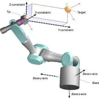
o A tip. The tip is always a dummy and is the last object in the considered kinematic chain (when going from the base to the tip). The tip dummy should be linked to a target dummy and the link should be an IK, tip-target link type. Refer also to the dummy properties.
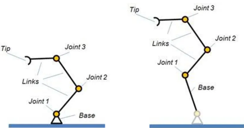
Figure 4.1: Two kinematic chains, each describing an IK element
IK Elements are specified by a kinematic chain (Figure 4.1), and a target to follow. The kinematic chain itself is specified by a tooltip (or end effector, or tip in short), indicating the last object in the chain, and a base, indicating the base object (or first object) in the chain. Above figure shows two kinematic chains as specified for an IK element. The IK element perceives the two chains in a similar way (the very first joint of the second example is ignored by the IK element).
In above example, the kinematic chains as specified by the tip/base pair, both have 3 Degrees of Freedom (DoF) because 3 1-DoF joints are involved. Should one of the joints however be a spherical joint, then the chain would have 5 DoF since a spherical joint has 3 DoF by itself.
mechanism (the specified kinematic chain) should move towards the target. This is the most basic case of IK task.
Figure 4.2: IK element and corresponding model of the IK solving task
Following are the steps to successfully set-up IK or FK calculations:
o Specify individual kinematic chains by providing a base and a tip.
o Specify a target to follow (simply link the tip dummy to a target dummy).
o Group IK elements in a single IK Group if they share common joints. o Order individual IK Groups in order to obtain the wanted behavior.
o Verify that joints in a kinematic chain have the correct properties enabled or disabled.
o Verify that individual IK Elements are not overconstrained (X, Y, Z, Αlpha-Beta, Gamma).
there are DoFs in the mechanism). Positional constraints are most of the time specified relative to the base's orientation as can be seen from following figure:
Figure 4.3: IK chain and constraints
mind that damping will always slow down the IK calculations (more iterations will be needed to put the tip into place).
Figure 4.4: IK task menu and options
Solving the FK problem of simple kinematic chains is trivial (just apply the desired joint values to all joints in the chain to obtain the position and orientation of the tip or end effector). It is less trivial to solve the IK and FK problem for closed mechanisms.
For our platform, we start with determining the collision free workspace. We attach both left and right jaco arms to a dummy base of about same height as actual platform and cycle through all possible joint space configurations excluding the ones leading to self-collision. The end effector position and orientation for these candidate configurations are stored and also displayed on the simulation screen. Doing this provides us with a much required constraint of collision free end effector work space.
Once this is done, we now have a workspace for motion planning. Next step is to create an IK group for our robot arm and perform simple inverse Kinematics. We use stationary base of jaco arm as our IK chain base while we create a Dummy object in the gripper to act as tip of our IK chain.
Figure 4.6: IK chain in Jaco arm
As seen in figure 4.6, we have a red dummy target along with our jaco arm IK chain. This target has a child script associated with it, connecting it to the tip of jaco IK chain. Hence one may either manually move the target (by clicking and dragging with mouse) or define a path for its travel in the child script, the end result will be Jaco arm will inverse kinematically follow the target, as long as it is in its workspace. Hence,
IK chain base
Dummy Target
while defining its motion path we use the data from previous experiment about workspace determination, to avoid singularity.
4.1.2
Precise Object Tracking
For precise control of camera movement, we carried out an object tracking experiment in V-REP motion planning. As described in the last section, we had an IK chain setup for the right jaco arm and a target dummy object for the arm to follow. For the purpose of proper visibility and effectiveness of our tracking, we added a laser pointer on the tip of jaco arm which should point towards object of interest if the tracking algorithm works successfully.
These angles are determined using following relationship between the end points of line segment between target dummy and object of interest:
𝛾 = 𝑎𝑡𝑎𝑛2(
𝑂𝑏𝑗𝑒𝑐𝑡(𝑦)−𝑇𝑎𝑟𝑔𝑒𝑡(𝑦) 𝑂𝑏𝑗𝑒𝑐𝑡(𝑥)−𝑇𝑎𝑟𝑔𝑒𝑡(𝑥))
𝛽 = 𝑎𝑡𝑎𝑛2(
𝑂𝑏𝑗𝑒𝑐𝑡(𝑥)−𝑇𝑎𝑟𝑔𝑒𝑡(𝑥) 𝑂𝑏𝑗𝑒𝑐𝑡(𝑧)−𝑇𝑎𝑟𝑔𝑒𝑡(𝑧))
𝛼 = 𝑎𝑡𝑎𝑛2(
𝑂𝑏𝑗𝑒𝑐𝑡(𝑧)−𝑇𝑎𝑟𝑔𝑒𝑡(𝑧) 𝑂𝑏𝑗𝑒𝑐𝑡(𝑦)−𝑇𝑎𝑟𝑔𝑒𝑡(𝑦))
Where α, β, and γ are euler angles that represent a sequence of three elemental rotations, i.e. rotations about the axes of a coordinate system. First rotation about z by an angle α, second rotation about x by an angle β, and last rotation again about z, by an angle γ.
For ease of implementation we convert these euler angles into quaternions. The reason for this is, V-REP API contains functions that utilize quaternions more often.
q1= sin(β/2)* sin(γ/2)* cos(α/2)+ cos(β/2)* cos(γ/2)* sin(α/2)
q2= sin(β/2)*cos(γ/2)*cos(α/2)+ cos(β/2)*sin(γ/2)* sin(α/2)
q3= cos(β/2)*sin(γ/2)*cos(α/2)- sin(β/2)*cos(γ/2)*sin(α/2)
q4= cos(β/2)*cos(γ/2)*cos(α/2)- sin(β/2)*sin(γ/2)*sin(α/2)
Every iteration, for a given position of the target dummy (based on path planning script), its orientation is calculated as above and then using that position and orientation data, jaco arm inverse kinematically tracks the object of interest. This is true even if the object of interest moves in the 3D space, the only constraint is the speed of object. If it is moving faster than specific threshold, the jaco arm lags behind in terms of tracking. This is due to the fact that for the simulation it takes a finite amount of time to execute each iteration, this depends on number of scripts being executed, the type of functions used in those scripts (some functions take more simulation time compared to the others), and amount of rendering. Other than that it also depends on the amount of change in jaco joint configuration space. For instance, if the arm has to change 3 joint angles from position 1 to 2 it will take more time compared to say changing 1 joint angle from position 2 to 3. After taking all these factors into account, the system still works great for our application as we are not tracking an object in 3D space but simply following a predefined trajectory for moving the camera from one configuration to another.
4.1.3
Final Framework Simulation
Figure 4.9: Final platform simulation
Our scene now consists of:
Entire hardware platform model with exact same dimensions as the actual hardware.
Miniature mobile robots disguised as cars.
And a giant cat travelling along for some reason.1. We start the environment as shown in figure 4.9 and the jaco arm moves to its intial position (Figure 4.10).
2. Then the target dummy moves across the track at five different equidistant positions, pausing at each for a small duration (to allow the time for
capturing images).
3. Once a time frame has been recorded, the system moves forward, the cars move a little and so does the husky base.
4. Again the system as a whole pauses and jaco arm goes to step 2.
5. This continues for specific number of iterations or until the platform reaches end of the track.
Figure 4.9 has the visibility layer for husky platform removed for showing clear trajectory. The arm moves through 5 positions across the track marked by blue dots, following the straight line trajectory defined by red line.
At each end effector configuration and for each time frame, the joint space configuration is recorded in a csv or text file, along with Husky wheel motor positions, for batch transfer to ROS which will further use this motion planning data to drive the actual hardware platform and acquire images.
4.2 ROS Framework
Once V-REP provides motion planning data for husky and jaco, ROS takes over for execution of actual platform. Figure 4.11 provides a flow chart representation of the process of image acquisition using ROS. The packages described in chapter 3 along with a custom package named image_acquisition created by us are used for robot control and data acquisition. The Kinect depth camera is registered to the RGB camera prior to usage by following the method described at [34]. As shown in the figure 4.11, once we have motion planning data in text/csv format following steps are taken:
messenger_node in image_acquisition package reads the data and creates a new text file where each time frame has following format:
* Left motor position Right motor position
jaco_config_1 jaco_config_2 jaco_config_3 jaco_config_4 jaco_config_5
reader_node in image_acquisition package reads this file and activates other nodes from packages described in chapter 3.
Once desired motor positions are reached, reader_node activates jaco_demo/joint_angle_workout node in jaco_arm_driver package. This node takes in joint angle configuration and moves the jaco arm accordingly.
Again reader_node checks whether a configuration has been reached by jaco_arm or not. Once it reaches that configuration, reader_node activates depth_node, disparity_node, and rgb_node under image_acquisition package. These nodes subscribe to respective topics published by openni_launch, read in image data and then convert them to png images using OpenCV (cv_bridge nodelet).
Chapter 5
Ground Segmentation
Segmentation is the process of partitioning a digital image into multiple segments (sets of pixels). The goal of segmentation is to simplify and/or change the representation of an image into something that is more meaningful and easier to analyze. [43, 8] Image segmentation is typically used to locate objects and boundaries (lines, curves, etc.) in images. More precisely, image segmentation is the process of assigning a label to every pixel in an image such that pixels with the same label share certain characteristics.
The idea of segmentation is crucial to autonomous driving. Ideally, we want to clearly separate out and identify cars, pedestrians, other vehicles, or obstacles in order to guarantee a reliable motion planning implementation. The first step towards this goal is to identify and isolate the ground/road from the image which in most driving situations is a major portion of the scene. An algorithm that can segment the ground in (ideally) real time is desirable to obtain location data between vehicles simultaneously executing autonomous drive.
to calculate its intrinsic and extrinsic parameters that define its internal geometry, and helps provide a relation between 3D world coordinates and 3D camera coordinates.
Figure 5.1: Pseudo colored disparity map [3]
5.1 RANSAC for Plane fitting
Originally proposed by Fischler et. al [17] in 1981 as a method for best fitting a model to a set of points, such as finding a 2D line that best fits through a set of x and y data points, RANSAC has become a vital technique for the Computer Vision field, owing to its accuracy and performance [6]. This technique can be easily extended to take a data set of 3D points and calculate the plane model that best fits the selection. Research [42] on a mobility aid for the partially sighted uses RANSAC to great effect – enabling best fit of the visible ground plane from disparity values, even when there are obstacles in the way. In a similar manner, research by Konolige et. al [27] into mapping and navigation of outdoor environments relied on RANSAC for finding the ground plane in a challenging terrain filled with obstacles (see Figure 5.2).
This robustness to obstacles is useful to our proposed method, as roads and highways generally contain obstacles like cars, pedestrians, etc. At the same time a considerable amount of image area is ground, facilitating RANSAC. The limitations of this technique are in its trade-off between accuracy and performance, based off how much of the ground plane is visible within the image frame when the calculation was processed. If very little of the ground plane is visible during calculation, then RANSAC will be unable to find a suitable plane that fits best with the data available. To overcome this, we select a small region closer to vehicle with a lower disparity value as candidate ground pixels. If it remains unable to find a sufficient plane after a few retries, it could then take the best model it was able to get from those attempts [29].
This approach allows us to combine the plane detection and calculation into a single step, providing a ground plane that can be related to the autonomous driving data.
5.2 Ground segmentation using RANSAC
The basic idea, as described in previous section, is to estimate the model parameters using minimum possible data and then to check which of the remaining data points fit the model estimated. Further, we can apply region growing to merge the neighboring planes within certain local range.
Following are the implementation steps for our RANSAC ground plane fitting algorithm:
2. To further reduce the time complexity, we uniformly sample these candidate pixels by a specific interval. This interval is decided by training the algorithm on any given environment over a few images by increasing the sampling interval until we strike a balance between execution time and performance. One such example of the points used for fitting is shown in Figure 5.3.
3. Create a test plane from three randomly chosen points of the initial pool. Ax+By+Cz+D = 0
Where, (A, B, C) is the nonzero normal vector of the plane through the point (x, y, z).
4. Test the remaining points in the pool against this fitted plane and count number of inliers based on minimum threshold distance. Keep a track of the plane estimation with maximum inliers.
5. Repeat steps 2 and 3 for a given number of iteration (we use 1000 iterations). If the plane with highest number of inliers crosses a threshold (70% of selected pixels) that plane is considered the ground plane.
6. If no plane has more inliers than the threshold, the process is continued until a plane with more inliers than the threshold is found.
7. Once a plane has been deemed as the ground plane, a least square fit is performed on the inliers for best approximation.
After computation of the ground plane, the obstacle pixels are computed as the pixels above the ground plane. The segmentation result of Figure 5.3 is shown in Figure 5.4 (Bottom), while Figure 5.4 (Top) shows the ground plane obtained by using RANSAC.
Chapter 6
Kinect View Validation Framework (KVVF)
Kinect View Validation Framework (KVVF) is a MATLAB based framework with GUI for processing and analyzing image sets acquired using the technique described in chapter 4. In addition to this, the framework also integrates direct means of testing techniques and algorithms for autonomous driving or image processing in general. We will use the plane fitting based ground segmentation technique to show the capabilities of this framework. We used MATLAB to create a graphical user interface using GUIDE. Later we wrote callback functions to interact with the GUI, these callback functions would in turn call other mathematical and image processing functions to achieve desired tasks. Figure 6.1 shows blank GUI with classification.
6.1 High Level Operation
To better understand the user level working of the application, a brief description is provided followed by the appropriate screen-shots. Every time Kinect View begins with a blank environment (Figure 6.1). The GUI is divided into various sections:
1. Frame/path selection
Inside each such folder lies a folder for each jaco configuration which in turn contains RGB, depth, and disparity images. For instance, if our platform moved to 10 different locations and at each location the arm moves to 5 different positions then we will have 10 parent directories containing 5 child directories each. And hence Kinect View will have a 10x5 Frame/path selection section (Figure 6.2).
Figure 6.1: Kinect View front end; 1: Frame/path selection; 2: Path display; 3: image view window; 4: options
2. Path display
selected path will be displayed with red dots connected via a line, while inactive frames will be displayed as black dots (Figure 6.2).
3. Image view window
This is a matlab implementation of image_view node from openni_launch package of ROS. It basically displays RGB and depth images for selected frame from section 1 in case of single view mode. For path selection mode, it shows depth and RGB images corresponding to last frame in selected path (Figure 6.3). 4. Options
This is the section where user makes selections about the mode of execution and controls the analysis. Currently this section provides a radio button to toggle between Single View mode and Path Selection mode (Figure 6.3). Refresh button is a global reset for this application and necessarily brings it back to initial blank stage. Random button selects a random path from time frame 1 to last time frame, this is extremely useful for quickly testing any algorithm on a subset of data from a large dataset. Details of implementation are in next section. Extract button extracts and loads data pertaining to selected frame/selected path (based on mode of operation selected) for further analysis and testing of techniques. Finally Gnd_Seg button performs RANSAC based ground segmentation discussed in chapter 5 on the extracted data set and stores result in a specific folder called processed_data. These results can be loaded into the image viewer window for quick analysis.
The Gnd_Seg button is modular and replicable. It can be easily replaced by a drop down menu to allow multiple algorithms/techniques to be a part of this framework. As discussed before there are two basic modes of data analysis:
1. Single View mode 2. Path Selection mode
Figure 6.2: Kinect View front end; 1: Frame/path selection; 2: Path display; Path Selection mode ON
Figure 6.3: Kinect View front end; 3: image view window; 4: options with Single View mode On
segmentation on the selected subset. The image view window displays segmented ground and obstacles for the last selected frame.
At any point during this operation, one may hit the refresh button to restart the entire pipeline from scratch. The results of ground segmentation are stored in a directory named processed_data in sequential order based on respective time frame.
6.2 Low Level Operation
After getting a look at the overall working of Kinect_View, this section goes down to the low level back end operations of the application. There are three basic components:
MATLAB GUI
Callback functions for GUI elements
Objective MATLAB scripts
The GUI has been created using MATLAB GUIDE, which is a pick and place type GUI wizard. Using GUIDE facilitates quick front end creation with fake buttons and elements. GUIDE automatically creates a matlab file containing callback function declarations for every interactive element in the front end scene.
Using those declarations we can either create function definitions in the same file or separate files. The callback function definitions contain program snippets which define and regulate the behavior of the front end upon interacting with respective elements. The properties of each element like name, value, enable state, etc. can be read and modified by accessing its handle. Hence in order to modify an element from within callback function of another element, one has to pass the handle of the element of interest to that callback function.
display window by updating the red and black dots and also changes the images loaded in the image view window.
Mode selection radio button has been assigned a global signal in its callback function, thus affecting all the other callback functions to make them behave according to the mode selected. The Random button is implemented by a two dimensional constrained random walk. Consider the frames as vertices of a graph, first vertex is chosen at random from the first time frame. After this we random walk across the graph until we reach the final time frame. The constraints include: no backtracking and not to traverse more than one vertex in any given time frame.