Neutrality Tests Using DNA Polymorphism From Multiple Samples

(1)



Neutrality Tests Using DNA Polymorphism From Multiple Samples

Haipeng Li,*

,†

_{Yunwu Zhang,}

†

_{Ya-Ping Zhang}

†

**_{and Yun-Xin Fu*}**

,‡,1

‡_{Laboratory of Bioinformatics, Yunnan University, Kunming 650991, People’s Republic of China,}_*_{Human Genetics Center,}

University of Texas, Houston, Texas 77030 and†_{Laboratory of Molecular Evolution and Genome Diversity, Kunming}

Institute of Zoology, Chinese Academy of Sciences, Kunming 650223, People’s Republic of China

Manuscript received April 23, 2002 Accepted for publication November 21, 2002

ABSTRACT

The polymorphism of a gene or a locus is studied with increasing frequency by multiple laboratories or the same group at different times. Such practice results in polymorphism being revealed by different samples at different regions of the locus. Tests of neutrality have been widely conducted for polymorphism data but commonly used statistical tests cannot be applied directly to such data. This article provides a procedure to conduct a neutrality test and details are given for two commonly used tests. Applying the two new tests to the chemokine-receptor gene (CCR5) in humans, we found that the hypothesis that all mutations are selectively neutral cannot explain the observed pattern of DNA polymorphism.

STATISTICAL TESTS

T

HE amount and pattern of polymorphism in DNA

sequence samples from a population reflects not _{A number of statistical tests can be extended for} multi-only mutations in the ancestors of the sequences but _{ple samples. However, for the sake of discussion, we} also random genetic drift as well as other evolutionary _{focus on two particular tests partly because they are} forces, such as natural selection. How to detect the pres- _{used widely. First,}_Tajima _{(1989) proposed using the} ence of natural selection in molecular population genet- _{difference between two estimates of}_␪ ₍_⫽₄_N_␮_{), where} ics and evolution is an important issue. It is possible to _N_{is the effective population size, and}_␮_{is the mutation} detect the presence of natural selection because natural _{rate per sequence per generation, to detect the presence} selection often causes the pattern of polymorphism to _{of selection. His test statistic is}

differ from that under the neutral mutation hypothesis, which postulates that the majority of mutations that

DT⫽ 兿⫺

K/an

√

Var(兿⫺K/an)

, (1)

have contributed significantly to the genetic variation in natural populations is neutral or nearly neutral (Kimura

where⌸is the mean number of nucleotide differences 1983). However, the neutral mutation hypothesis is not

between two sequences,Kis the number of segregating sufficiently quantified to be tested rigorously in practice.

sites, which is equal to the total number of mutations A narrower definition of neutrality is that all mutations

under the infinite-sites model,nis sample size, and are selectively neutral, which is referred to as the

hypothe-sis of strict neutrality(FuandLi1993).

an⫽1⫹

1

2⫹. . . ⫹ 1

n⫺ 1. (2)

A number of statistical tests have been proposed, and almost all of them are designed for a single sample. In

reality, polymorphic data can be accumulated over time _Second, _Fu _and _Li _{(1993) suggested several tests of} in the same or different laboratories, which means dif- _{neutrality, one of which is}

ferent sites may be examined using different samples.

How to conduct neutrality tests in such situations is the _D

F⫽

K⫺an␰1

√

Var(K⫺ an␰1)

, (3)

focus of this article. To date, millions of single nucleo-tide polymorphisms (SNPs) have been identified. It is

where ␰1 is the number of mutations in the external

very likely that SNPs from a single gene or tightly linked

branches, that is, mutations that are inherited by only regions will be typed for different samples by different

one sequence in the sample. research groups over time. The newly developed

The above two tests can be extended to multiple sam-method will be valuable for analyzing such data. We

ples in the following way. Assume that a locus without present an example of such an analysis using data from

recombination is divided intomregions that have been theCCR5 gene.

surveyed using different or partially overlapping sam-ples (Figure 1). It should be emphasized that the as-sumption of no recombination is made here to make the

1_{Corresponding author:}_{Human Genetics Center, UT School of Public}

null model as simple as possible, similar to the original Health, P.O. Box 20186, 1200 Herman Pressler, Houston, TX 77030.

E-mail: [email protected] Tajima and Fu and Li tests. Just as the presence of

(2)

⌸ ⫽

兺

m

i⫽1

⌸i, (4)

K⫽

兺

m

i⫽1

Ki, (5)

and

␰1 ⫽

兺

m

i⫽1

␰1i. (6)

It is obvious that whenm⫽ 1, these equations reduce to their conventional definitions for a single sample. Note that in these equations the same weight is given to every region. An alternative approach is to give weight to a region according to certain criterion. However, so far we have not found any other weighting scheme to perform better than the equal-weighting scheme.

Figure1.—An illustration of a genealogy of multiple

sam-Furthermore, we define ples. The locus is divided into two regions. The sequence

length in the first region is 400 and in the second one is 600,

a ⫽

兺

m

i⫽1

rian_i, (7)

so r1⫽0.4 andr2⫽ 0.6 under the hypothesis of a constant

mutation rate. |S1|⫽3, |S2|⫽3, andS1傽S2⫽{3}. That means

{1, 2} are sequenced from 1 to 400, {4, 5} are sequenced from _where_a

n_iis given by (2). That is,ais a weighted average

401 to 1000, and {3} is sequenced from 1 to 1000. The subtree

ofan_i. Then the tests (1) and (3) become

for the first region is marked by solid lines, and the subtree for the second region is labeled by dashed lines. The lengths

of branches can be calculated from coalescent times, and the _D

T⫽

⌸ ⫺K/a

√

Var(⌸ ⫺K/a) (8) length of a branch here means a time duration. For example,

g⫽t2⫹t3⫹t4, andh⫽t2. LetLibe the branch length of

the subtree for theith region, and thenL1⫽ a⫹b⫹g⫹ and

h⫹ e, andL2⫽ c⫹ d⫹ f⫹ e. The branch of eis shared

among two subtrees.lkiis the length of the k-size branch in _D

F⫽

K⫺ a␰1

√

Var(K⫺a␰1)

. (9)

the subtree for theith region, sol11⫽a⫹b⫹h⫹e,l21⫽g,

l12⫽c⫹d⫹e, andl22⫽f. Five mutations are on the genealogy

and are shown as circles, three of which (solid circles) are found in the first region, and two of which (shaded circles)

are found in the second region. Therefore,␰11⫽2, ␰21⫽1, PERFORMING THE TESTS

␰12⫽2, and␰22⫽0.

Since Var(⌸ ⫺ K/a) ⫽ Var(⌸) ⫹ Var(K)/a2 ⫺ ₂

Cov(⌸, K)/a and Var(K ⫺ a␰1) ⫽ Var(K) ⫹ a2 Var

(␰1)⫺2aCov(K,␰1), we can compute Var(⌸ ⫺K/a) and

recombination does not invalidate the Tajima and Fu Var(K⫺a␰1) if we are able to compute Var(K), Var(⌸),

and Li tests, but makes them more conservative, the Var(␰1), Cov(⌸,K), and Cov(K,␰1). Some of these terms

new tests will likely behave similarly and this will also can be computed analytically; others have to be

esti-be applicable to data with recombination. _mated.

Define ␪ ⫽ 4N␮, where ␮ is the mutation rate per _{Analytical result:}_{Assume the total sample consists of} sequence per entire locus, andNis the effective popula- _n_{sequences, and let those sequences be numbered from} tion size. Also define␪i⫽4N␮i, where␮iis the mutation 1 ton.S⫽{1, 2, . . . ,n} will represent the whole sample.

rate for theith region (i⫽1, 2, . . . ,m), andri⫽ ␮i/ The sample,Si, for theith region will be a subset ofS.

␮, which is the proportion of the mutation rate of the That is Si 債 S. We do not make any assumption here

ith region. If the mutation rate per site is constant, the on the relationship amongSi. We note that in one

ex-ri is equal to the proportion of the length of the ith treme, we can haveS_i傽 S_j⫽ φfor every pair of iand

region, j, and on the other hand, we may haveS1⫽S2⫽. . .⫽

Sm ⫽ S. In many situations, it is likely thatSi 傽 Sj ⬆φ

兺

m

i⫽1

ri ⫽1 . (e.g., Figure 1). We use |S_i| to represent the number of

elements in the setSi, which is the sample size. Then

we haveni⫽ |Si|,n⫽|S|.

Furthermore, we define the mean number of nucleotide

differences between two sequences in theith region as The computation of Var(⌸), Var(K), and other com-ponents that we mentioned above requires

understand-⌸i, the number of segregating sites in theith region as

Ki, the number of mutations in the external branches ing of the sample genealogy. LetLibe the total branch

length of subtree for theith region scaled so that 1 unit of the genealogy in theith region as␰1i, and the sample

(3)

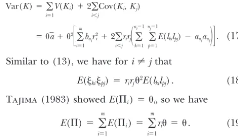
branch here means a time duration.␰kiis the number Var(K)⫽

兺

m

i⫽1

V(Ki)⫹2

兺

i⬍j

Cov(Ki,Kj)

ofk-size mutations in theith region, andlkiis the length

ofk-size branches in the subtree for theith region scaled

⫽ ␪a⫹ ␪2

冤

兺

m

i⫽1

bnir

2

i ⫹2

兺

i⬍j

rirj

冢

兺

ni⫺1

k⫽1

兺

nj⫺1

p⫽1

E(lkilpj)⫺anianj

冣冥

. (17)

similarly as Li (Figure 1). The size of a branch is the

number of sequences in the sample that are descendants

Similar to (13), we have fori⬆jthat of that branch, and a mutation is said to besize kif it

occurs in a branch of sizek(Fu1995). Considering the _E₍_␰_ki_␰_pj₎_⫽ _r_i_r_j_␪2_E₍_l

kilpj) . (18)

subtree that is part of the tree shown as solid lines in

Tajima(1983) showedE(⌸i)⫽ ␪i, so we have

Figure 1, the branch ofghas 2 descendent sequences, 1 and 2, so the size of the branch is 2. A mutation is

E(⌸)⫽

兺

m

i⫽1

E(⌸i)⫽

兺

m

i⫽1

ri␪ ⫽ ␪. (19)

on the branch of g, so the size of the mutation is 2. Following the definition of␪,␪i, andri, we have

Since⌸iis the mean number of nucleotide differences

␪i ⫽4N␮i⫽ 4N␮(␮i/␮)⫽ri␪. (10) between two sequences in theith region, it can be

calcu-lated from␰kias

Moreover, since 1 unit in time corresponds to 4N gener-ations, we have fromLiandFu(1998)

⌸i ⫽

2

ni(ni⫺1)

兺

ni⫺1

k⫽1

(ni⫺k)k␰ki (20)

E(Li)⫽ani. (11)

(Fu1995).Tajima(1983) derived the variance of⌸ias

Under the infinite-sites model, we have

Var(⌸i)⫽

ni⫹1

3(ni⫺1)

ri␪ ⫹

2(n2

i ⫹ni⫹ 3)

9ni(ni⫺ 1)

r2

i␪2. (21)

E(K)⫽

兺

m

i⫽1

E(Ki)⫽

兺

m

i⫽1

␪iE(Li)⫽ ␪a. (12)

So we have Conditioning on the coalescent times, the number of

mutations in each branch follows a Poisson distribution E(⌸i⌸j)⫽E

冤

2

ni(ni⫺1) 兺

ni⫺1

k⫽1

(ni⫺k)k␰ki

2

nj(nj⫺1) 兺

nj⫺1

p⫽1

(nj⫺p)p␰pj

冥

with parameter␪l, wherelis the branch length. We thus have

⫽ 4␪2

ninj(ni⫺1)(nj⫺1)

冤

兺 n_i⫺1

k⫽1 兺

n_j⫺1

p⫽1

kp(ni⫺k)(nj⫺p)rirjE(lkilpj)

冥

,

E(KiKj|t2,t3, . . .)⫽ ␪iLi␪jLj ⫽rirj␪2LiLj, ₍₂₂₎

and thus wheretk(2ⱕkⱕ n) is the time duration required for

ksequences to coalesce tok⫺ 1 sequence,i.e., the

so-Var(⌸)⫽

兺

m

i⫽1

Var(⌸i)⫹2

兺

i⬍j

E(⌸i⌸j) ⫺2

兺

i⬍j

[E(⌸i)E(⌸j)] ,

calledk-coalescent time (Figure 1), andi⬆j. Then we

have ₍₂₃₎

E(KiKj)⫽Et2,t3,…,tn[E(KiKj|t2,t3, . . . ,tn)]⫽rirj␪

2_E₍_L

iLj) , where Var(⌸_i) andE(⌸_i⌸_j) are given by (21) and (22),

(13) respectively. Moreover, from (12) and (19), we have

Cov(K,⌸)⫽E(K⌸)⫺E(K)E(⌸)⫽E(K⌸)⫺ ␪2_a_,

which leads to

(24) Cov(Ki,Kj)⫽E(KiKj)⫺E(Ki)E(Kj)⫽rirj␪2[E(LiLj)⫺anianj] .

where E(K⌸) is given later (Equation 25).Fu (1995) (14)

showed the formula to calculateE(␰ki␰pi). After putting

these terms together, we have Watterson(1975) showed that Kin the case of one

sample is

E(K⌸)⫽E

冢

兺

m

i⫽1

Ki

兺

m

i⫽1 ⌸i

冣

⫽

兺

m i,j

E

冤冢

兺

ni⫺1

k⫽1 ␰ki

冣冢

2

nj(nj⫺1)

兺

nj⫺1

p⫽1

(nj⫺p)p␰pj

冣冥

Var(Ki)⫽an_i␪i⫹bn_i␪2i ⫽an_iri␪ ⫹bn_ir2i␪2, (15)

⫽

_兺

m

i⫽1

兺

ni⫺1

k⫽1

兺

ni⫺1

p⫽1

2(ni⫺p)p

ni(ni⫺1)

E(␰ki␰pi)

where

⫹ ␪2

兺

i⬆j

兺

ni⫺1

k⫽1

兺

nj⫺1

p⫽1

2(nj⫺p)p

nj(nj⫺1 )

rirjE(lkilpj) . (25)

bn⫽ 1⫹

1

4⫹ . . .⫹ 1 (n⫺ 1)2.

Also we can partitionE(LiLj) further as _From_Fu_{(1995), we have}

E(LiLj)⫽ E

冢

兺

n_i⫽1

k⫽1 lki

兺

n_j⫺1

p⫽1 lpj

冣

兺

n_i⫺1

k⫽1

兺

n_j⫺1

p⫽1

E(lkilpj) . (16) E(␰ki)⫽

1

k␪i, (26)

(4)

TABLE 1

E(␰1)⫽

兺

m

i⫽1

E(␰1i)⫽

兺

m

i⫽1

␪i ⫽ ␪ (27)

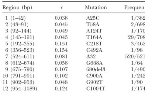
The list ofriand the frequencies of mutations in 12 regions of theCCR5 gene

and

Region (bp) r Mutation Frequency

Var(␰1)⫽Var

冢

兺

m

i⫽1

␰1i

冣

⫽

兺

m

i⫽1

Var(␰1i)

1 (1–42) 0.038 A25C 1/382

2 (43–91) 0.045 T58A 2/698

⫹2

兺

i⬍j

Cov(␰1i,␰1j). (28)

3 (92–144) 0.049 A124T 1/170

4 (145–191) 0.043 T164A 29/708

FuandLi(1993) showed that the variance of the total

5 (192–355) 0.151 C218T 3/462

number of mutations in the external branches is given _{6 (356–523)} _0.154 _C492A _1/98

by _{7 (524–611)} _0.081 _⌬32 _520/5210

8 (612–674) 0.058 G668A 1/64

Var(␰1i)⫽ ␪i ⫹cni␪2i, (29)

9 (675–790) 0.107 680del3 1/490

10 (791–901) 0.102 C900A 1/242

wherecn⫽ 1 whenn ⫽2, and whenn⬎ 2

11 (902–953) 0.048 G902T 1/90

12 (954–1089) 0.124 C1004T 1/174

cn⫽2

nan⫺2(n⫺1)

(n⫺1)(n⫺ 2). _CCR_{5 mutations and their frequencies in Caucasians come}

from Carrington et al. (1997), and the frequency is the

From (18) and (26), we have

number of alleles observed/the total number of chromo-somes.

Cov(␰1i,␰1j)⫽E(␰1i␰1j)⫺E(␰1i)E(␰1j)

⫽rirj␪2E(l1il1j)⫺rirj␪2. (30)

Substituting (29) and (30) into (28), we have

the estimation can be improved by using large values ofM.

Var(␰1)⫽

兺

m

i⫽1

(ri␪ ⫹cnir2i␪2)⫹2

兺

i⬍j

(rirj␪2E(l1il1j)⫺rirj␪2),

The components mentioned above can be obtained (31) after E(lkilpj) is estimated, and then DT and DF can be

and calculated. Similar toTajima’s(1989) andFuandLi’s

(1993) tests,DT andDFdo not follow well-known

stan-Cov(K,␰1)⫽ E

冢

兺

m

i⫽1

Ki

兺

m

j⫽1

␰1j

冣

⫺ E(K)E(␰1) dard distributions. Since E(lkilpj) have to be estimated

from simulated samples, it is natural to use computer simulations to determine the critical points of the tests.

⫽

_兺

m

i⫽1

兺

ni⫺1

k⫽1

E(␰ki␰1i)⫹ ␪2

兺

i⬆j

兺

ni⫺1

k⫽1

rirjE(lkil1j)⫺ ␪2a,

Overall, this approach gives more accurate critical values (32) than using approximation by a standard distribution.

whereE(␰ki␰1i) is given byFu(1995).

Numerical estimation: The above derivation shows _{AN EXAMPLE}

that E(lkilpj) is critical for computing Var(K), Var(⌸),

We consider data from theCCR5 gene from Cauca-Cov(⌸,K), Var(␰1), and Cov(K,␰1). The value ofE(lkilpj)

sians (Carrington et al. 1997) to illustrate how the is dependent on the relationship of branches among

extended tests described in this article can be applied. subtrees of the regions. A simple example of the

rela-The CCR5 encodes a cell-surface chemokine-receptor tionship is given in Figure 1. Although Fu (1995) was

molecule that serves as a co-receptor for the macro-able to derive E(lkilpj) wheni ⫽ j, the general formula

phage-tropic strains of HIV-1. Because of its obvious fori⬆jappears to be analytically intractable. However,

importance, theCCR5 gene has been subjected to many an estimate can be obtained relatively easily from the

studies. One hypothesis is thatCCR5 might have been following procedure:

under natural selection (Carrington et al.1997). In 1. Simulate a genealogyg(topology without mutation) _{the data from}_Carrington_{et al.}_{(1997), 12 mutations} of a sample ofn sequences numbered from 1 ton. _{were documented in Caucasians, and 10 of the} discov-2. Compute the value ofEg(lkilpj) for the simulated gene- ered mutations alter the amino acid sequence of the

alogy. _{protein, and each mutation is typed by different or}

3. Repeat steps 1 and 2Mtimes. ThenE(lkilpj) is finally partially overlapping samples (Table 1). Since the

pre-estimated as _{cise relationships among samples were not given in the}

original article, we consider two extreme cases here.

Eˆ(lkilpj)⫽

1

M

兺

g

Eg(lkilpj). In the first case, we assume that different samples are

composed of different individuals. That is,Si傽Sj⫽ φ,

wherei⬆ j. In the second case, we assume that smaller The computation ofEg(lkilpj) in step 2 is done in a similar

(5)

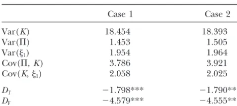
TABLE 2 cant negative values in both cases 1 and 2. Thus we conclude that the CCR5 region has not evolved

ac-Results of neutrality tests forCCR5

cording to the neutral model. One possibility is that it has evolved under natural selection, which remains to

Case 1 Case 2

be seen by further study.

Var(K) 18.454 18.393

We are grateful to Ms. Sara Barton for her help. This work is

Var(⌸) 1.453 1.505

supported by National Institutes of Health grants R01 GM50428 and

Var(␰1) 1.954 1.964

R01 GM55759 (Yun-Xin Fu), the Chinese Academy of Sciences

Cov(⌸,K) 3.786 3.921

(KSCX2-1-05), the National Nature Science Foundation of China, and

Cov(K,␰1) 2.058 2.025

the Nature Science Foundation of Yunnan Province in China.

DT ⫺1.798*** ⫺1.790***

DF ⫺4.579*** ⫺4.555***

LITERATURE CITED Statistical significance was calculated from the empirical

distribution ofDT andDF. ForDT, the critical values for the Carrington, M., T. Kissner, B. Gerrard, S. Ivanov, S. J. O’Brien

et al., 1997 Novel alleles of the chemokine-receptor geneCCR5.

1% significance tests are⫺1.663 (case 1) and⫺1.660 (case 2),

Am. J. Hum. Genet.61:1261–1267. and forDFthe values are⫺2.829 (case 1) and⫺2.631 (case 2).

Fu, Y. X., 1994 Estimating effective population-size or mutation-rate The values are estimated from 10,000 simulated samples.

using the frequencies of mutations of various classes in a sample ***The test result is significant at 1% level.

of DNA sequences. Genetics138:1375–1386.

Fu, Y. X., 1995 Statistical properties of segregating sites. Theor. Popul. Biol.48:172–197.

S8(64)傺S11(90)傺S6(98)傺S3(170)傺S12(174)傺S10 Fu, Y. X., andW. H. Li, 1993 Statistical tests of neutrality of

muta-tions. Genetics133:693–709. (242)傺S1(382)傺S5(462)傺S9(490)傺S2(698)傺S4

Kimura, M., 1983 The Neutral Theory of Molecular Evolution. Cam-(708)傺S7(5210), where the numbers in parentheses are _{bridge University Press, Cambridge, UK.}

Li, W. H., andY. X. Fu, 1998 Coalescent theory and its applications the sample sizes. We refer to those two cases as case 1

in population genetics, pp. 45–79 inStatistics in Genetics, edited and case 2, respectively. By assuming samples are

inde-by E.Halloran. Springer-Verlag, New York.

pendent in the first case, we basically obtain the maxi- _{Tajima, F}_{., 1983} _{Evolutionary relationship of DNA sequences in} finite populations. Genetics105:437–460.

mum possible information from such data. On the other

Tajima, F., 1989 Statistical method for testing the neutral mutation hand, by assuming smaller samples are a subset of larger

hypothesis by DNA polymorphism. Genetics123:585–595. samples, we have the minimal amount of information. Watterson, G. A., 1975 On the number of segregating sites in

genetic models without recombination. Theor. Popul. Biol.7: From (12), we can get the estimate of ␪ as ␪ˆ⫽K/a,

256–276. sincea⫽6.274, so we have␪ˆ_⫽1.913. Also we have⌸ ⫽

(6)