A Model-Based Method for Identifying Species Hybrids Using Multilocus Genetic Data



A Model-Based Method for Identifying Species Hybrids Using

Multilocus Genetic Data

E. C. Anderson

1

_{and E. A. Thompson}

Department of Statistics, University of Washington, Seattle, Washington 98195 Manuscript received October 3, 2001

Accepted for publication December 24, 2001

ABSTRACT

We present a statistical method for identifying species hybrids using data on multiple, unlinked markers. The method does not require that allele frequencies be known in the parental species nor that separate, pure samples of the parental species be available. The method is suitable for both markers with fixed allelic differences between the species and markers without fixed differences. The probability model used is one in which parentals and various classes of hybrids (F1’s, F2’s, and various backcrosses) form a mixture

from which the sample is drawn. Using the framework of Bayesian model-based clustering allows us to compute, by Markov chain Monte Carlo, the posterior probability that each individual belongs to each of the distinct hybrid classes. We demonstrate the method on allozyme data from two species of hybridizing trout, as well as on two simulated data sets.

H

YBRIDIZATION between individuals from genet- from a sampled population belonging to the six

genea-ically distinct populations is of interest across logical classes of parentals, F1’s, F2’s, and backcrosses

many fields within biology. Hybrid zones, regions where that are the possible first- and second-generation

prod-individuals from genetically distinct populations inter- ucts of all possible matings between two species. To

breed to form genetically mixed offspring, have been employ their method, individuals in the sample must

recognized as fertile grounds for evolutionary studies be classified exclusively to one of the six categories or

concerning models of speciation, selection, recombina- be excluded from the analysis altogether because they

tion, the maintenance of species boundaries, and the fall into the “ambiguous” category. This requires that

evolution of host-parasite interactions (Hewitt 1988; parental species can be sampled separately, so that the

BoecklenandSpellenberg1990;Harrison1990). In frequency of different alleles among the parentals may

conservation biology and resource management, hy- be estimated and then used as if known without error.

bridization between endemic species and introduced Additionally, it requires that each parental species be

species (Goodman et al. 1999) or between wild and segregating for unique alleles, though even then it is

cultured populations (Elo et al. 1995; Jansson and not always possible to unambiguously assign individuals

Oest1997) is a topic of great concern. to the different categories.EpifanioandPhilipp(1997)

Mendelian genetic markers (Avise1994) provide valu- note that error rates when classifying individuals to

hy-able tools for studying species hybridization because brid categories may be quite high if few loci are available.

they allow the characterization of individuals as pure- This is so even with diagnostic loci: loci that are fixed

bred individuals or hybrids. Such a characterization is for alternate alleles in the different species.Boecklen

useful, if not crucial, to the research goals in many andHoward(1997) give expressions and

recommen-studies of hybridizing populations. For example, identi- _{dations for the number of markers needed to achieve}

fying individuals as belonging to pure, F1, F2, or back- a desired level of classification error, under several

crossed classes is important for documenting gene ex- _{restrictive assumptions such as unidirectional}

backcross-change and introgression between species. _{ing and diagnostic loci.Miller(2000) provides a}

simi-Several methods have been advanced for identifying _{lar analysis describing the probability of}

misclassifica-hybrid individuals (CamptonandUtter1985;Nason _{tion using diagnostic dominant markers.}

and Ellstrand 1993; Barton 2000; Miller 2000; _{Other methods for identifying hybrids with genetic}

Younget al.2001). One family of methods relies on the _{data do not necessarily require that the different species}

use of alleles that are unique to each species.Nason _{possess unique alleles.CamptonandUtter(1985)}

de-andEllstrand(1993) present a maximum-likelihood _{rive a statistic that is a simple function of the conditional}

method for estimating the proportion of individuals _{probability of an individual’s genotypes at multiple loci}

given the parental species’ allele frequencies. Once again, this method requires that the parental allele

fre-1_{Corresponding author:Department of Integrative Biology, University}

quencies are already known separately from the sample

of California, Berkeley, CA 94720-3140.

E-mail: [email protected] of hybrids. And further, this method allows only for the

resolution of individuals into pure and hybrid categories putational framework that may be easily adapted to spe-cial cases.

and does not indicate directly whether individuals are

Our method is related to the method ofRannalaand

F1, F2, or backcrossed hybrids.Barton(2000) suggests

Mountain (1997), but differs substantially in that it that, rather than classifying hybrids into genealogical

treats all the individuals in a sample simultaneously, classes, they could be classified by the number of alleles

rather than on a one-by-one basis. Our method also is derived from each taxon and the number of

heterozy-similar to Pritchard et al.’s (2000) Bayesian method

gous loci they possess. He suggests a moment-based

for analyzing structured populations. However, their method for doing such classification using the

informa-method focuses on a genetic inheritance model speci-tion implicit in the linkage disequilibrium present in

fied in terms of the proportion of an individual’s ge-hybridizing populations.

nome originating from each of a set of possible subpop-The above methods for classifying hybrids require that

ulations. This is a useful heuristic model for populations the allele frequencies of each species are known or

with structure of unknown origin; however, when popu-can be estimated separately. When it is not possible to

lations are known to consist of pure individuals and sample the different species separately and hence obtain

recent hybrids of two species, a more detailed analysis estimates of the parental allele frequencies, the

classifi-using an inheritance model defined in terms of

geno-cation of hybrids is more difficult.Younget al.(2001)

type frequencies, as pursued here, is possible. recently demonstrated the use of principal coordinate

In this article, we assume that we have a sample of analysis (a general multivariate statistical technique) to

individuals drawn from a hybridized population and cluster pure individuals of two species of trout and their

genotyped atLunlinked loci. We describe the

popula-hybrids. Individuals intermediate between the two

spe-tion model and the genetic model for hybridizaspe-tion and cies clusters were assumed to be hybrids. These were

then describe the likelihood function that these models removed from the sample before estimating allele

fre-imply. We then describe how that likelihood is used in quencies in the parental species. This method of

separat-a Bseparat-ayesiseparat-an specificseparat-ation of the problem separat-and how Mseparat-arkov ing hybrids from pure individuals has the drawback that

chain Monte Carlo (MCMC) is carried out for simulat-the principal coordinate analysis is not based upon a

ing from the Bayesian posterior distribution. Once the genetic model, so the clusters are not readily

interpret-method is developed, we apply it to multilocus genetic able, and, further, the parental allele frequencies so

data from juvenile steelhead trout (Oncorhynchus mykiss),

obtained are made under the assumption that the

classi-cutthroat trout (O. clarki clarki), and hybrids of the two

fication of hybrids by the principal coordinate analysis

species collected from a coastal stream in Washington is correct.

state. We then demonstrate the method on two simu-We present a new Bayesian statistical method for

iden-lated data sets and discuss the results. One data set has tifying hybrids. Rather than assigning individuals to a

many relatively uninformative markers and the other single hybrid category, our method computes the

poste-has nearly diagnostic markers. Finally, in the discussion, rior probability that an individual in the sample belongs

we note several useful extensions that could be easily to each of the different hybrid categories. This posterior

handled within the framework described here. probability reflects the level of certainty that an

individ-ual belongs to a hybrid category. This is an improvement

over previous methods, which do not explicitly compute PROBABILITY MODEL AND

COMPUTATIONAL METHODS

the probability of misclassification of particular

individ-uals. It further allows the inference of all model parame- _{Genotype frequency classes:We consider a group of}

ters to be made while integrating over the uncertainty _{individuals in the wild that consists of sympatric}

popula-in hybrid category classifications, rather than makpopula-ing _{tions of two species, A andB, and hybrids of the two}

those inferences conditional on a single classification _{species that have occurred fromnpotential generations}

of individuals to hybrid or pure categories. Our method _{of interbreeding. We take nto be known or assumed.}

also has the following attractive features: (1) It is based _{For example, it may be known that speciesAwas}

intro-upon a genetic model, so the results are easily interpre- _{ducedngenerations ago to speciesB’s range, or it may}

ted; (2) it does not require that parental classes be _{be that the hybrids have reduced fitness, so hybrids}

sampled separately, though if they can be, then those _{remaining in the population will be hybridized for no}

samples can be included as prior information in the _{more than n generations. More practically, it is well}

model; (3) it does not require that loci be diagnostic, _{known that individuals arising from many generations}

or even that the species possess unique alleles—it can of backcrossing are difficult to distinguish from pure

make use of the information in frequency differences individuals even with many diagnostic markers (Boecklen

between alleles that are not fixed in either species; (4) andHoward1997); hence the quality of the data limits

it incorporates the uncertainty due to the fact that allele the extent of the biological inferences one can make.

frequencies are always estimated and are not known With few markers or with low genetic differentiation

com-cies at the top of the pedigree. Since there are 2n

found-ers for a pedigree withngenerations, there are 2n⫹₁

different gene frequency classes that are determined by

the number,a, of founders originating from the species

Apopulation (a ⫽ 0, 1, . . . , 2n_{). In Figure 1, both c}

and f belong to the gene frequency class witha ⫽ 2.

The individuals at the bottoms of the other pedigrees belong to the remaining four distinct gene frequency classes.

We use uppercaseQto denote the proportion of an

individual’s genome derived from the speciesA

popula-tion. This quantity, which we refer to as the “genetic heritage proportion,” is discrete and is determined by the gene frequency class to which an individual belongs,

namely Q ⫽ a/2n_{, with a defined as in the previous}

Figure1.—Six arrangements of founders on a pedigree of

n⫽2 generations. Each box represents a locus. The circles paragraph. We note thatQis the quantity estimated by

within each box represent the two genes possessed by the _{BartonandGale’s (1993) familiar hybrid indexzand} diploid organism at the locus. The founders are the individuals _{also thatQ is closely related to the latent variable q}(i) k

in the top row of each pedigree. Black gene copies are those

described in the model with admixture developed by

originating from the speciesApopulation, and the white genes

Pritchard et al. (2000) as the proportion of the

ge-are from speciesB.Genes that are not determined to be either

black or white by the pedigree and the founders in it are nome of theith individual originating from population

denoted by broken circles. The individual at the bottom of _{k. Q is necessarily discrete in our approach since we} each pedigree belongs to a different hybrid class, determined

perform the analysis conditional uponn, the number

by the arrangement of species among the founders. a–f

repre-of generations repre-of potential interbreeding. By contrast

sent six distinctgenealogical classes.a–f also represent six distinct

q(i)

k is used as a continuous variable byPritchardet al.

genotype frequency classes.There are, however, only five distinct

gene frequency classes; the individuals at the bottoms of pedigrees (2000), although they do treatq(i)

k as a discrete variable

c and f are both in the same gene frequency class. _{in their model for detecting immigrants with prior}

pop-ulation information. ThePritchardet al.(2000) model

for detecting immigrants is similar to what we propose

between all the hybrid categories generated by as few _{here for detecting hybrids; however, their model is}

re-asn⫽2 orn⫽3 generations of potential interbreeding. _{stricted to the case where the number,a, of immigrant}

When hybridization between two species has been _{founders on a sampled individual’s pedigree does not}

potentially occurring for n generations, the possible _{exceed one, and it does not make use of the expected}

genealogical classesinto which an individual may fall can _{frequencies of single-locus genotypes that we discuss}

be enumerated and described by considering the possi- _below.

ble arrangements of different species among the found- _{With gene frequency classes and the genetic heritage}

ers in an n-generational pedigree, up to changes in _{proportion so defined, it is straightforward to}

enumer-branching order at any node in the binary tree of the _{ate and define the genotype frequency classes. The}

pedigree. The individual of interest is taken to be the _{members of a genotype frequency class all have the}

member at the bottom of the pedigree and is assumed _{same expected proportion of single-locus genotypes}

to be noninbred over the lastngenerations; hence we _{possessing 0, 1, or 2 genes originating from speciesA.}

assume there are no loops in itsn-generational pedigree. _{For the}

gth genotype frequency class we denote these

Figure 1 illustrates this for the case ofn⫽2. With data _{expected proportions by}

Gg ⫽ (Gg,0, Gg,1, Gg,2),

respec-only on unlinked loci, it is not possible to resolve all _{tively. Enumerating these genotype frequency classes}

the genealogical classes for n ⱖ 3. For example, the _{and computing the expected proportions of the}

geno-expected proportions of different multilocus genotypes _{types follows from Mendel’s laws. Since each individual}

composed of unlinked markers for the F2and F3genea- _{receives one gene copy randomly selected from the two}

logical classes are identical. Instead, with unlinked _{in its mother and another randomly selected from the}

marker data, one can only resolve what we refer to as _{two in its father, the expected proportions of the}

geno-genotype frequency classes. _{types in an individual are determined by the gene}

fre-Before describing genotype frequency classes, how- _{quency classes to which its parents belong. For thegth}

ever, it is convenient to consider a simpler classification _{genotype frequency class, we have}

of hybrid individuals intogene frequency classes.Members

of the same gene frequency class have the same ex- Gg,0 ⫽(1⫺ Qm)(1⫺ Qf)

pected proportion of all their genes originating from

Gg,1 ⫽Qm(1⫺ Qf)⫹Qf(1 ⫺Qm)

speciesA.This is determined by the number of founders

whereQm andQfare the genetic heritage proportions from the speciesApopulation, and it takes the value 0

if that gene copy originated from species B. We use

of the individual’s mother and father (and the sexes

of the parents are interchangeable). Straightforward Wi⫽(Wi,1, . . . ,Wi,L) to denote all the latent gene origin

indicators in theith individual, andWdenotes the latent

algebra verifies that two individualsiandjwill belong

to the same genotype frequency class if and only if the gene origin indicators in all the individuals.

The allelic types of the two gene copies at locusᐉin

parents ofjbelong to the same gene frequency classes

as the parents ofi.Consequently, the number of distinct individualiare denoted byYi,ᐉ⫽(Yi,ᐉ,1,Yi,ᐉ,2), with each

ofYi,ᐉ,1 andYi,ᐉ,2taking an integer value between 1 and

genotype frequency classes afterngenerations of

possi-ble interbreeding can be calculated as the number of Kᐉ, inclusive, corresponding to the possible allelic types

at theᐉth locus. TheLsingle-locus genotypes in theith

unordered pairs that may be formed from the 2n⫺1 _⫹

1 gene frequency classes aftern⫺1 generations: (2n⫺1_{⫹ individual are denoted by Y}

i⫽ (Yi,1, . . . ,Yi,L), and all

1)(2n⫺1⫹_{2)/2. We denote this quantity by}Ᏻ

n. Fornⱖ of the genetic data over allMindividuals in the sample

2 there are always more genotype frequency classes than isY⫽(Y1, . . . ,YM). We introduce some notation here

there are gene frequency classes. With data on multiple to avoid awkward subscripting: let ␪A 具i; ᐉ; j典 denote

unlinked loci, it is possible to distinguish between indi- the frequency in the speciesApopulation of the allele

viduals in different genotype frequency classes. This is possessed by theith individual at thejth (j⫽1, 2) gene

our primary inference goal and will be pursued in the copy of itsᐉth locus. This is a shorthand for the doubly

Bayesian context by computing the posterior probability subscripted␪A,ᐉ,_Yi,ᐉ,j. We also introduce the latent variable

that each individual belongs to each of theᏳngenotype Zi: Zi ⫽ gindicates that individual iin the sample

be-frequency classes. The following section describes the longs to genotype frequency classg.

data and the probability model for making such infer- Given the population allele frequencies, the gene

ori-ence. gin indicators, and the genotype frequency class to

Genetic data and probability model:We have a sample which an individual belongs, it is easy to compute the

of M individuals drawn for genetic analysis. For now, probability of that individual’s single-locus genotype at

we assume that individuals are sampled randomly and theᐉth locus. For our purposes later, it is more useful

independently of whether they are purebred individuals to have an expression for the joint probability of the

of either species or are hybrids. This sort of sampling genotype and the gene origin indicators. At the ᐉth

would arise if, for example, the two species, or hybrids _{locus in individuali belonging to genotype frequency}

thereof, were difficult to distinguish on the basis of _{classg, this joint probability is}

morphology—so-called “cryptic” hybridization. Each

in-P(Yi,ᐉ,Wi,ᐉ|Zi ⫽g,␪A,ᐉ,␪B,ᐉ)

dividual in the sample is genotyped atLunlinked loci.

Let theᐉth locus possessKᐉalleles detected in the

sam-ple. We denote the allele frequencies in speciesAand

B,ngenerations ago, by⌰A and⌰B, respectively. Each

of these⌰’s is a collection of vectors, with each vector ⫽









␪A具i;ᐉ; 1典␪A具i;ᐉ; 2典Gg,2, ifWi,ᐉ,1 ⫽Wi,ᐉ,2⫽ 1 ␪A具i;ᐉ; 1典␪B具i;ᐉ; 2典Gg,1/2, ifWi,ᐉ,1 ⫽1,Wi,ᐉ,2⫽0 ␪B具i;ᐉ; 1典␪A具i;ᐉ; 2典Gg,1/2, ifWi,ᐉ,1 ⫽0,Wi,ᐉ,2⫽1 ␪B具i;ᐉ; 1典␪B具i;ᐉ; 2典Gg,0, ifWi,ᐉ,1 ⫽Wi,ᐉ,2 ⫽0.

giving the allele frequencies at a particular locus. For

example, for species A, ⌰A ⫽ (␪A,1, . . . , ␪A,L), where

(2)

␪A,ᐉ ⫽ (␪A,ᐉ,1,, . . . , ␪A,ᐉ,K_ᐉ) are allele frequencies at the

ᐉth locus. The alleles found in individuals from species _{The product of the two allele frequencies in the above}

A and species B are assumed to be drawn randomly _{expressions follows from the assumption that each gene}

from the allele frequencies⌰A and⌰B, respectively, n copy in the founders (n generations ago) of the ith

generations ago. Likewise, individualsngenerations be- _{individual is sampled randomly from the alleles present}

fore sampling are assumed to be in Hardy-Weinberg _{in its population of origin. Then,Gg,2is the probability}

and linkage equilibrium with reference to their contem- _{that an individual in genotype frequency classghas both}

poraneous conspecifics; thus, linkage disequilibrium _{gene copies originating from species A, G}

g,1/2 is the

and Hardy-Weinberg disequilibrium in the mixed popu- _{probability that the first (second) gene copy originates}

lation are assumed to result entirely from the mixing and _{from species Aand the second (first) originates from}

admixing of the gene pools of speciesAand speciesB. _{species B, and G}

g,0 is the probability that both gene

Within an individual, the two gene copies carried at _{copies originated from speciesB.}

any locus are considered to be ordered and indexed by _{For a given genotype frequency class, the marginal}

prob-j ⫽ 1 or 2. The order of the gene copies is arbitrary; _{ability of theith individual’s genotype at locusᐉis}

com-for example, it may merely be the order in which the _{puted by summing (2) over the latent gene origin}

indi-genetic data on that locus in that individual happened _cators:

to be recorded. We do not know from which species

P(Yi,ᐉ|Zi⫽ g,␪A,ᐉ,␪B,ᐉ)⫽

兺

0ⱕ_Wi,ᐉ,1ⱕ1 0ⱕWi,ᐉ,2ⱕ1

P(Yi,ᐉ,Wi,ᐉ|Zi⫽ g,␪A,ᐉ,␪B,ᐉ).

each of an individual’s gene copies descended, but we denote that unknown information by the latent variable

Wi,ᐉ⫽(Wi,ᐉ,1,Wi,ᐉ,2).Wi,ᐉ,jtakes the value 1 if thejth gene

Finally, under the assumption of unlinked markers in choice facilitates simulation from the full conditional

distributions for⌰Aand⌰B. The Dirichlet distribution

Hardy-Weinberg and linkage equilibrium among

con-specificsn generations ago, the probability of the ith is also the multivariate generalization of the beta

distri-bution, which arises theoretically as the equilibrium dis-individual’s multilocus genotype is just the product over

theLsingle-locus genotype probabilities: tribution for gene frequencies in the presence of genetic

drift and linear pressure from migration or mutation

P(Yi|Zi⫽g,⌰A,⌰B)⫽

兿

L

ᐉ⫽1

P(Yi,ᐉ|Zi⫽g,A,ᐉ,␪B,ᐉ). (4) (Wright1938, 1952). Specification of the parameters

␭A,ᐉ ⫽ (␭A,ᐉ,1, . . . , ␭A,ᐉ,K_ᐉ) and␭B,ᐉ ⫽ (␭B,ᐉ,1, . . . , ␭B,ᐉ,K_ᐉ)

provides a way to incorporate prior information about This gives us an expression for the probability of the

the allele frequencies among the two species at theᐉth

data on a single individual. We now must derive the

locus. If, at locusᐉ, previous studies have indicated that

probability of the data on allMindividuals in the sample.

speciesBhas very low frequency of allelejwhile species

We do this by modeling the hybridized population as a

Ahas high frequency, then␭B,ᐉ,jshould be chosen small,

mixture with unknown proportions of individuals from

relative to the other components of ␭B,ᐉ, while ␭A,ᐉ,j

the different genotype frequency classes.

should be chosen large. If, on the other hand, very little

As shown earlier, given n generations of potential

prior knowledge is available about allele frequencies in interbreeding between the species, the members of the

the two species, then a sensible choice of prior␭A,ᐉ,j⫽

genetic sample may fall into Ᏻn ⫽ (2n⫺1 ⫹ 1)(2n⫺1 ⫹

␭B,ᐉ,j⫽1/Kᐉforj⫽1, . . . ,Kᐉ. This has the form of the

2)/2 genotype frequency classes. We model the

individ-Jeffreys prior for a multinomial proportion (seeGelman

uals in the sample as being randomly and independently

et al.1996). drawn from a mixture of individuals, each belonging to

The conjugate prior for␲is also a Dirichlet

distribu-one of theᏳngenotype frequency classes with

probabil-tion, so it is helpful to letP(␲)⬅ Dirichlet (␨1, . . . ,

ity␲g,g⫽1, . . . ,Ᏻn,

兺

gᏳ⫽n1␲g⫽1. Using ␲to denote

␨Ᏻn). As with the allele frequencies, the parameters␨⫽

the vector of mixing proportions, (␲1, . . . , ␲Ᏻn), we

(␨1, . . . , ␨Ᏻn) could be specified so as to reflect prior

may now write the probability of all the observed data

knowledge of the biology of the situation. For example,

Yconditional onn,⌰A,⌰B, and␲as the product over

if it was well known that backcrosses between F1hybrids

theMmembers of the sample of the probability of each

and species A had low fitness, then that could be

re-of their multilocus genotypes:

flected in the prior for␲. Additionally, if hybridization

and backcrossing were known to be fairly rare, then this

P(Y|⌰A,⌰B,␲)⫽

兿

M

i⫽1

冢

兺

Ᏻn

g⫽1

␲gP(Yi|Zi⫽g,⌰A,⌰B)

冣

. (5)

prior knowledge could be reflected by having smaller

␨g’s for those genotype frequency classes that required

Assigning each genotype frequency class a separate

mix-more episodes of interbreeding within the lastn

genera-ing proportion provides a means of accountgenera-ing for

possi-tions. In the absence of prior information on hybridiza-ble differential fitness of the different classes.

tion rates, the prior␨g⫽1/Ᏻn,g⫽1, . . . ,Ᏻnis again

A Bayesian specification:Equation 5 is the likelihood

a suitable choice.

for⌰A,⌰B, and␲. To pursue Bayesian inference in this

The influence of prior distributions in this sort of

problem requires prior distributionsP(⌰A),P(⌰B), and

hierarchical model is not easy to predict, and

determin-P(␲), so that the posterior distribution may be

com-ing a good prior distribution to use in the absence

puted. We wish to make inferences not only about⌰A,

of prior information is not a simple task (Kass and

⌰B, and␲, but also the latent variablesWandZ⫽(Z1,

Wasserman1996). A second reasonable choice of prior

. . . ,ZM), so we are concerned with the joint posterior

is the uniform Dirichlet distribution—␭A,ᐉ,j ⫽ ␭B,ᐉ,j ⫽ 1

distribution, which is proportional to the joint

probabil-forj⫽1, . . . ,Kᐉor␨g⫽1,g⫽1, . . . ,Ᏻn. However,

ity of all the variables,P(Y,⌰A,⌰B,␲,Z,W). With the

this uniform prior represents a substantial amount of latent variables present, this joint density factorizes as

information when the number of components is large

(for example, if Kᐉor Ᏻn is large). For this reason we

P(Y,⌰A,⌰B,␲,Z,W)⫽P(⌰A)P(⌰B)P(␲)

prefer the use of the previously described Jeffreys-type

⫻

_兿

M

i⫽1

P(Yi|Wi,⌰A,⌰B)P(Wi|Zi)P(Zi|␲), priors, which reflect the amount of information

con-tained in a single observation, rather than inKᐉor Ᏻn

(6)

observations. Because of the fact that some of the

geno-which, as we see in the next section, allows straightfor- type frequency classes will have few if any members in

ward MCMC sampling from the posterior distribution, the sample, and because some alleles will be found only

P(⌰A,⌰B,␲,Z,W|Y). in low frequency in either of the species, there is

poten-It is computationally convenient and biologically rea- tial that the posterior will be sensitive to the choice of

sonable to take the specific form of the prior distribu- prior. We used various combinations of the uniform

tions⌰Aand⌰Bto be Dirichlet distributions, indepen- and Jeffreys-type priors in analyzing the data sets

de-dent over theLunlinked loci. That is,P(␪A,ᐉ) is Dirichlet scribed later in the article and found that, although

(␭A,ᐉ,1, . . . ,␭A,ᐉ,K_ᐉ). Since the Dirichlet distribution is the there were differences in some of the specific posterior

alter the conclusions made from the analysis based on gene copies of allelic typejfor which the corresponding

W·,ᐉ,·⫽1). An analogous expression exists forP(␪B,_ᐉ|···).

the Jeffreys-type priors.

MCMC simulation from the posterior distribution:It The full conditional distribution for␲is also easily com-puted by conjugacy as

is not possible to compute directly the posterior distribu-tions for only the variables that we are interested in.

P(␲|···)⬅Dirichlet(␨1⫹s1, . . . ,␨Ᏻn⫹ sᏳn), (8)

However, simulating from the joint posterior

distribu-tion of all the variables by MCMC can be done via Gibbs where sg is the number of individuals in the sample

sampling in a manner similar to that for normal finite currently allocated to genotype frequency classg.The

mixture models (Diebolt and Robert 1994). Gibbs full conditional distribution for the pair of gene origin

sampling is a special case of theHastings(1970) algo- indicators Wi,ᐉ in theith individual currently included

rithm for constructing an ergodic Markov chain having in thegth genotype frequency class is obtained by Bayes’

a unique stationary distribution for which the normaliz- law as

ing constant may be unknown. In this case, the desired

stationary distribution is the posterior distribution of all P(Wi,ᐉ|···)⫽P(Yi,ᐉ,Wi,ᐉ|Zi ⫽g,␪A,ᐉ,␪B,ᐉ)

P(Yi,ᐉ|Zi⫽g,␪A,ᐉ,␪B,ᐉ)

, (9)

unknown variables in the model and is known up to

scale (i.e., without knowing the normalizing constant) _{where the numerator and denominator are given in}

by Equation 6. Given initial starting values for all the _{(2) and (3), respectively. Finally, the full conditional}

variables in the model, Gibbs sampling proceeds by suc- _{distribution for Z}

i would be P(Zi|Wi, ␲). However, it

cessively simulating new values for particular variables _{is possible to integrate out the W}

i conditional on the

in the model from their full conditional distributions (Ge- _{remaining variables and hence simulate new values of}

manandGeman1984). After a sufficient period of burn- _Z

i from P(Zi|Yi, ⌰A, ⌰B, ␲), instead of from P(Zi|Wi,

in, a sample of variables drawn from this joint posterior _{␲). This is an example of improving MCMC efficiency}

distribution allows Monte Carlo estimation of the poste- _{through “collapsed Gibbs sampling” (Liu1994). In our}

rior distribution of any subset of variables of interest, _{case, this is particularly attractive, since computing}

either marginally or conditional on the values taken by _P(Z

i|Yi, ⌰A, ⌰B, ␲) incurs almost no extra cost—the

another subset of variables. _{quantities needed to calculate it have already been}

com-We denote full conditional distributions by P(·|···) _{puted in step 3 of the sweep. By Bayes’ law}

and refer to a standard iteration of our MCMC

algo-rithm as a “sweep.” A sweep consists of a series of steps _P(Z

i⫽ z|Yi,⌰A,⌰B,␲)⫽ ␲

zP(Yi|Zi⫽ z,␪A,␪B)

兺

Ᏻn

g⫽1␲gP(Yi|Zi⫽g,␪A,␪B)

, in which each of the variables in the probability model

(except for the data, Y, which are fixed) is updated

z ⫽1, . . . ,Ᏻn. (10)

once. Here, with the probability distributions given in

more detail below, the steps in a single sweep are as Multiple chains are run from different starting values

to diagnose mixing problems. In this case, it is easy to follows:

assign overdispersed starting values by simulating values

1. Forᐉ⫽ 1, . . . ,L, simulate new values for ⌰A,ᐉand _{of ⌰}

A, ⌰B, and␲from their prior distributions rather

⌰B,ᐉfromP(⌰A|···) andP(⌰B|···), respectively. _{than their full conditional distributions in steps 1 and}

2. Simulate a new value of␲fromP(␲|···). _{2 of the first sweep. We usedGelman’s (1996) estimated}

3. Fori⫽1, . . . ,Mandᐉ⫽1, . . . ,L, simulate a new _{scale reduction potential factor to monitor convergence}

value ofWi,ᐉfromP(Wi,ᐉ|···). _{of the chains to the desired posterior distribution. This}

4. Fori ⫽1, . . . ,M, simulate a new value ofZifrom _{quantity is computed for each scalar variable in the}

P(Zi|Yi,⌰A,⌰B,␲). _{posterior distribution. For each such variable, the}

poten-tial scale reduction is computed as the square root of By sampling the current states of all the variables after

the ratio of the variance of the variable estimated by each sweep, one acquires a dependent sample suitable

using information from all of the multiple chains to the for Monte Carlo estimation of most quantities of

inter-variance of the variable estimated by using the values est. In particular, a Monte Carlo estimate of the

poste-simulated from just a single one of the chains. Values

rior probability that individuali is of thegth genotype

of the scale reduction potential near 1 indicate that the frequency class is obtained by averaging the values of

chains have converged to the target distribution.

P(Zi ⫽g|Yi,⌰A,⌰B,␲) computed during each sweep.

In the case of data from cutthroat trout and steelhead The full conditional distributions are easily derived.

trout described in the following section this conver-By conjugacy,

gence occurs very rapidly. Burn-in then requires little

P(␪A,ᐉ|···)⬅Dirichlet(␭A,ᐉ,1⫹rA,ᐉ,1, . . . ,␭A,ᐉ,K_ᐉ⫹rA,ᐉ,K_ᐉ), time. This will typically be the case for genetically

well-separated species. Poor mixing of the Markov chain may (7)

occur for species that are not genetically well separated.

Pritchardet al.(2000) discuss strategies for specifying

where rA,ᐉ,j is the number of gene copies of allelic type

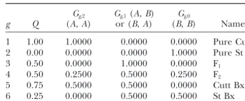
mix-TABLE 1

ing in such cases. However, it is likely that with genetic

differentiation low enough to have mixing problems _{Genotype frequency classes assumed for the analyses}

with the MCMC, it will be very difficult, if not impossible,

to distinguish most genotype frequency classes. _{Gg,2 Gg,1(A,B) Gg,0}

g Q (A,A) or (B,A) (B,B) Name

1 1.00 1.0000 0.0000 0.0000 Pure Cutt ANALYSIS OF THREE DATA SETS

2 0.00 0.0000 0.0000 1.0000 Pure St

We demonstrate our method by analyzing one real _{3 0.50 0.0000 1.0000 0.0000 F1}

and two simulated data sets. The real data consist of 74 4 0.50 0.2500 0.5000 0.2500 F2

5 0.75 0.5000 0.5000 0.0000 Cutt Bx

juvenile trout from Whiskey Creek, Washington state,

6 0.25 0.0000 0.5000 0.5000 St Bx

typed at 30 polymorphic protein loci, having between

two and four alleles, as part of a large genetic survey _{These are the six genotype frequency classes that arise from}

conducted by the National Marine Fisheries Service and _n⫽ 2 generations of potential interbreeding.Gg,2, Gg,1, and

Gg,0are the expected frequencies of loci having 2, 1, or 0 genes

the Washington Department of Fish and Wildlife. The

originating from speciesA, as described in the text. The final

sample was collected under the belief that the fish were

column gives names that we use to refer to these genotype

juvenile coastal cutthroat trout (O. clarki clarki);

how-frequency classes.

ever, the Hardy-Weinberg and linkage disequilibrium in the sample, and the presence of homozygotes for

alleles common in steelhead trout (O. mykiss) popula- . . . , 6 for the mixing proportions,␲, of the different

genotype frequency classes. A total of 100,000 sweeps tions but rare in cutthroat trout populations, suggested

that the sample might be a mixture of cutthroat, of five chains started from overdispersed starting values

were run. This required 4.6 hr on a laptop computer steelhead, and their hybrids. Hybrids between these two

trout species have been documented in several rivers on with a 266 Mhz G3 (Macintosh) processor.

After applying the method to the Whiskey Creek data

the West Coast (CamptonandUtter1985;Neillands

1990). set, we demonstrate its use on simulated data sets 1 and

2. Data set 1 is a simulated set of steelhead and cutthroat

The report ofJohnsonet al.(1999) gives more details

about the sampling and the genotyping of the trout. It trout data. To simulate data set 1, we started with two

species having allele frequencies at 30 unlinked loci that also summarizes the available literature from the field

and the laboratory on hybridization between O. clarki were the posterior mean estimates of allele frequencies

in the cutthroat and steelhead populations at the 30

clarkiandO. mykiss.They report that there are no severe

developmental abnormalities that occur in hybrids of loci used in the analysis of the Whiskey Creek data. We

simulated a sample of size 300 individuals with 155 pure the two species; hybrid offspring are clearly viable.

How-ever, hybrids may possess morphological and behavioral cutthroat (Pure Cutt), 100 pure steelhead (Pure St),

25 F1, 6 F2, 14 cutthroat backcross (Cutt Bx), and 0

steel-traits that reduce their fitness in natural environments.

This accords well with the observation in other studies head backcross (St Bx) individuals. This sort of sample

might be encountered from a population in which that hybrid individuals are detected typically among

ju-venile trout, but adult hybrids are seldom observed, and steelhead and cutthroat hybridize infrequently, and the

F1’s tend to mate assortatively, being more likely to mate

with the observation that although hybridization may

occur each year (in cases where it has been monitored with other F1’s or with pure cutthroat than with

steelhead. To simulate theith individual belonging to

over time it has been found to be ongoing) the two

species still remain distinct. Nonetheless, in some stud- thegth genotype frequency class, the species origin of

each gene copy at a locus was randomly assigned ac-ies, the fish sampled and analyzed possess genotypes

suggesting they belong to a hybrid class involving more cording toGg, and then the allelic type of each gene was

randomly selected from its species of origin according to than just one generation of hybridization. Here, we

apply our method to the genetic data from Whiskey the posterior mean allele frequencies estimated from

the Whiskey Creek analysis. Creek with particular reference to the task of

distin-guishing between F1and later hybrids. Simulated data set 2 is a sample of 300 individuals

with the same number of individuals belonging to the For this analysis, we assume there are six genotype

frequency classes to which individuals might belong— different genotype frequency classes as in data set 1.

However, data set 2 consists of 20 nearly diagnostic loci

the six classes arising fromn⫽2 generations of potential

interbreeding. Table 1 lists the expected proportions for distinguishing the two simulated species, Aand B.

That is, there are assumed to be 20 diallelic, codominant of the different single-locus genotypes in these six classes

and also gives the names that we use to refer to them. loci at which the frequency of the first allele is 0.995 in

species A and the frequency of the alternate allele is

Though prior information is available on allele

frequen-cies in other steelhead and cutthroat populations, we 0.995 in species B. This represents considerably more

power to distinguish species than is present in the trout

do this analysis using the prior␭ᐉ,j⫽1/Kᐉ,j⫽1, . . . ,

Figure2.—Graphical summary of results for the Whiskey Creek data set. (a) The 20 probable Pure St individuals appear as solid circles while the 50 probable Pure Cutt fish appear as open circles in the graph with the height of the circles determined by the posterior probability of being Pure St or Pure Cutt, respectively. The four remaining fish are plotted on the graph as open trian-gles at heights given by the posterior proba-bility that they are either Pure St or Pure Cutt. The fish are ordered by their posterior probability of being purebred. (b) Posterior probabilities of genotype frequency class for fish 19, 48, 16, and 72—the four plotted as triangles in a. The height of the different patterns in the column denotes the poste-rior probability of each fish belonging to each of the six different genotype frequency classes.

Both of the simulated data sets were analyzed assum- Cutt. All of the fish with posterior probability ⬎0.8 of

being Pure St have negligible posterior probability of

ingn ⫽2 and using the same priors on the allele

fre-quencies and the mixing proportions that were em- being Pure Cutt and vice versa. Of the remaining 4 fish,

3 of them, nos. 19, 48, and 16, have posterior probability ployed in the analysis of the Whiskey Creek data. Five

chains, started from overdispersed starting points, were ⬍0.01 of being either Pure Cutt or Pure St. This means

that, given the data and the assumptions of the model simulated for 45,000 sweeps each. This required 8 hr

for data set 1 and 5.3 hr for data set 2 on the same 266 and the priors used, those fish have probability ⬎0.99

of being hybrids of some sort. The fourth fish (no. 72) Mhz G3 processor.

has posterior probability near 0.12 of being either Pure Cutt or Pure St; hence, posterior probability near 0.88

RESULTS

of being a hybrid of some sort. Figure 2 graphically represents this.

Whiskey Creek data:Using the multilocus genotype

data on the 74 fish in the data set, our method success- We may look more closely at the four probable hybrid

fish. Figure 2b shows the posterior probabilities that

fully estimated allele frequencies⌰Aand⌰Bfor the two

putative species contributing to the sample. Inspecting fish 19, 48, 16, and 72 belong to each of the six different

genotype frequency classes. Note that they all have high-these allele frequencies, it was clear that one set of

frequencies corresponded to the steelhead group and est posterior probability of belonging to the F2 class.

This is unexpected because one would suspect there the other to the cutthroat group, so we were able to

label them as such. In this analysis, each fish is assigned would be, in general, more F1’s in a population than

F2’s since the F2’s would have to be formed by mating

a posterior probability of belonging to one of the six

different genotype classes. Two of those classes are pure- between F1’s. In fact, the posterior probabilities for all

these fish are such that no classification or assignment bred categories (Pure Cutt and Pure St). Twenty of the

fish in the sample have posterior probability ⬎0.8 of of any of them could be made with great certainty to a

single one of the genotype frequency classes. As already being in the Pure St category, and for 15 of those fish,

that posterior probability is⬎0.99. Fifty fish have poste- noted, with posterior probability 0.12, fish 72 may

be-long to the Pure St category. Further, it cannot be

deter-rior probability ⬎0.8 of being Pure Cutt, with 45 of

Figure3.—Histograms showing the posterior distribution of allele frequencies estimated for the steelhead and cutthroat populations in Whiskey Creek. The solid symbols are for alleles in the steelhead population, and the open symbols de-note the cutthroat allele frequencies. The vertical axis in each graph is proportional to posterior probability density. The numbers 1–6 refer to dif-ferent loci ranked in order or how informative they are for distinguishing between the species. Locus 4 has three alleles, and the others have two alleles. Note that locus 1 is the only one that is close to being diagnostic. For a contrast, consider locus 6: The steelhead population has high poste-rior probability of being fixed for a single allele, but that allele is at a frequency around 0.4 in the cutthroat population.

F1hybrids. And even fish 16 has a posterior probability nostic locus. For all the others, there is almost zero

of almost 0.07 that it is an F1 hybrid. In other words, posterior probability that an allele appearing in the

no conclusions may be made with great confidence steelhead species does not appear in the cutthroat

spe-about the presence of fish in the sample that are hybrids cies or vice versa. Having such a small number of loci

belonging to categories beyond F1. This is due to the that are distinctive between the species makes it difficult

lack of clear separation between the two species in this to make fine-scale inferences about the specific

geno-data set. Only about eight of the loci are very informa- type frequency classes to which an individual belongs.

tive, and none of them are strictly diagnostic when infor- This point is made clear again by the analysis of the

mative priors for the allele frequencies are not used. first simulated data set.

A statistically reasonable way to measure the degree Simulated data set 1: This data set was simulated

as-to which a locus is useful in separating the species is by suming that allele frequencies in the two species were

the Kullback-Leibler divergence (KullbackandLeib- equal to the posterior mean estimates from the Whiskey

ler1951) between the two species at that locus. Briefly, Creek data set. In this case, since we know the true

at locusᐉthe Kullback-Leibler divergence between spe- _{genotype frequency classes to which each individual}

cies A and B is ᐀ᐉ(A, B) ⫽ Iᐉ(A:B) ⫹ Iᐉ(B:A), where belongs, we can better assess how well the method works

Iᐉ(A:B) is the expected Kullback-Leibler information for on this data set. Figure 4 shows how well purebred

indi-distinguishing the species from which an allele at locus _{viduals in the sample could be distinguished from the}

ᐉoriginated given that it came from speciesA.Mathe- _{hybrids. For most of the Pure Cutts and the Pure St the}

matically, for a given value of the allele frequencies, _{posterior probability or being in the correct genotype}

frequency class is⬎0.99. There are 32 Pure Cutts with

Ie(A:B)⫽

兺

K_ᐉ

k⫽1 ␪A,ᐉ,klog

␪A,ᐉ,k ␪B,ᐉ,k

. (11) posterior probability of being Pure Cutt⬍0.98. Almost

all of the remaining probability for these individuals goes to the Cutt Bx category. There are, in contrast,

By averaging the values of ᐀ᐉ(A, B) obtained for the

only seven Pure St individuals with posterior probability different allele frequencies visited by the Markov chain

of Pure St⬍0.98. This is most likely due to the fact that

in doing MCMC, it is possible to compute the posterior

there are no St Bx individuals in the sample, so the mean Kullback-Leibler divergence between the species

proportion of St Bx individuals in the population is at each locus. We have done this to identify the six most

estimated to be small, and hence even the fish that are informative loci in the data set, and we have plotted the

not well distinguished solely by their genotype between posterior distribution of the allele frequencies at those

the Pure St and the St Bx classes will tend to have a loci in Figure 3. From this figure, it is apparent that

Figure5.—Posterior probabilities of specific genotype fre-quency categories for the hybrid individuals in simulated data set 1. (a) Twenty-five simulated F1’s. (b) Six simulated F2’s and

14 simulated Cutt Bx’s, as indicated.

frequencies used in the simulations it is much more difficult to make clear distinctions between the different hybrid genotype frequency classes. Figure 5a shows the posterior probabilities of inclusion in the six genotype

frequency classes for the 25 F1 hybrids in descending

Figure4.—Results for simulated data set 1. (a) Posterior

probability of Pure Cutt for 155 simulated cutthroat trout. (b) order of the posterior probability that they are F1’s.

Posterior probability ofP(Pure St) for 100 simulated steelhead _{While many of them have high posterior probability of} trout. (c) Posterior probability of either Pure Cutt or Pure St

being F1, there is also one with posterior probability

for 45 simulated hybrid trout of genotype frequency classes

⬎0.5 of being in the Cutt Bx category. For the non-F1

denoted by the different symbols as given in the inset.

hybrids, the situation is even less promising. Of the six

F2individuals (the last six individuals in Figure 5b), not

one of them has posterior probability ⬎0.5 of being

This is a clear example of how the method gives weight

in the F2 category. Finally, for the Cutt Bx genotype

to the proportion of individuals from different genotype

frequency class, as the first 14 columns in Figure 5b frequency classes found in the sample. These results

reveal, there is a great deal of variability among the also suggest that, with data similar to those from Whiskey

individuals in the posterior probability that they are Creek and with many purebred individuals of each

spe-Cutt Bx. This results from having few loci in this simu-cies sampled, it is unlikely that any purebred individual

lated data set that are strongly distinctive between the will receive high posterior probability of being in a

non-species, and it argues that with genetic data of this sort, purebred genotype frequency category.

assignment of individuals, if desired, to specific geno-All but 1 of the 45 simulated hybrid fish have posterior

type frequency classes should be made with caution and

probability⬍0.20 of being either Pure St or Pure Cutt,

only in the presence of very strong posterior support

and 37 of them have posterior probability ⬍0.02 of

(for example,⬇0.98) of that assignment.

being purebred. As is apparent in Figure 4c, it is most

Simulated data set 2:The analysis with 20 nearly diag-difficult to distinguish the Cutt Bx’s from the purebred

nostic loci demonstrates how well the method performs

categories. As expected, the F1’s are the easiest to

distin-when the populations are genetically well separated by guish from the purebred individuals.

the markers. The 155 species A individuals, the 100

While the method works well in distinguishing

this method does not require that each species possess unique alleles.

We have demonstrated the method by analyzing data from cutthroat and steelhead trout. Though the data set includes 30 loci polymorphic in the sample, many of the loci are not very informative. Given only the 74 individuals in the sample, none of the loci appear to be purely diagnostic. While information from samples drawn from other steelhead and cutthroat populations could be used as prior information, we used a vague

Figure 6.—Posterior probability of genotype frequency _{prior on allele frequencies, reflecting little prior} knowl-classes for the 14 B Bx individuals and 6 F2 individuals in _{edge of allele frequencies, so as to demonstrate the}

simulated data set 2.

method’s performance with data having no apparently diagnostic loci. Despite such restricted data, the method was able to identify four individuals having high

poste-probabilities⬎0.9996 of belonging to the correct

geno-rior probability of being species hybrids.

type frequency class. Likewise, the six F2’s each had _{The analysis of data simulated to mimic the trout data}

posterior probability⬎0.997 of belonging to the F2ge- _{provides insight into the method’s ability to distinguish}

notype frequency class, and all but two of the simulated

between the different genotype frequency classes that

B Bx individuals had posterior probability ⬎0.997 of

the hybrids belong to. Despite the low level of genetic

belonging to theBBx class. As Figure 6 shows, of the

differentiation between the two trout species, the

poste-remaining twoBBx individuals, one has posterior

prob-rior probability of being purebred was very low for most

ability 0.983 of beingBBx; this individual possessed, by

of the simulated hybrids. However, it was clear that it random chance, many more loci heterozygous for the

is much harder to distinguish the specific (i.e., F2 vs.

two alleles than expected of aBBx. The remaining B

backcrossed category) genotype frequency classes of hy-Bx individual happened to be one of the rare carriers

brid individuals without many loci showing extreme

al-of a locus homozygous for the speciesAcommon allele.

lele frequency differences between the species. Our This can occur because the loci were designed in the

analysis of a simulated data set with 20 nearly diagnostic simulation to not be perfectly diagnostic. Our method

loci demonstrates the method’s ability to identify the is able to handle such a situation because it does not

specific genotype frequency of individuals with great require that loci are fixed for alternate alleles. The result

certainty using highly informative genetic data. is just that the posterior probability of belonging to the

A number of assumptions are made to derive the correct genotype frequency class is reduced for that

likelihood in this problem. One of the advantages of the individual.

model-based approach over a more general multivariate approach (like principal component analysis) is that the assumptions here are explicit. One important

as-DISCUSSION

sumption is that the loci used in the analysis are

un-We have developed a model-based statistical method linked. In studies with a limited number of loci on

for identifying species hybrids using multilocus genetic organisms with many chromosomes, this assumption is

data. Using Markov chain Monte Carlo in a Bayesian not likely violated. However, as the number of loci

in-setting, we compute the posterior probability that an creases, so does the probability that some of them will

individual belongs to each of a set of possible genotype be linked. Under the assumption of no linkage, each

frequency classes. This allows us to utilize all the data locus is treated as an independent unit of information;

simultaneously, while integrating over the uncertainty however, the information carried by linked loci will not

in individual assignments to genotype frequency classes be independent. Therefore, analyzing data on linked loci

and in the model parameters—the proportion of indi- with this method will cause one to overestimate one’s

viduals from the different genotype frequency classes certainty in identifying species hybrids. If the

recombina-and the allele frequencies of each of the species—which tion fractions between the markers were known, it would

are seldom known without error. This method also has be possible to account for linked loci. However,

model-the advantage that it can perform a mixture deconvolu- ing the dependence between loci in a manner faithful

tion withouta prioriknowledge of the allele frequencies to the underlying process could incur a heavy

com-in the separate species. In other words, one need not putational cost, and the use of an approximation, for

be able to separate the two species on the basis of mor- example, a Markov approximation to the genotype

fre-phology, nor must one be able to sample from the pure quency class process along the chromosome as taken

species separately, to separate the two species and their byMcKeigue (1998) in a related problem, would be

hybrids present in a mixture. Finally, though strong computationally preferable.

linked, this analysis assumes that the markers used are We adopted a simple sampling model: Individuals are assumed drawn at random from a population that is a not tightly linked to any loci that are under selection.

Especially with large numbers of markers, this assump- mixture in the proportions ␲ of individuals from the

different genotype frequency classes. This was probably

tion will be violated to an extent. For example,

Riese-bergandLinder(1999), reporting on hybrids between violated in the case of the cutthroat trout data, because, when the biologists collected the specimens, they were two sunflower species of known pedigree, find that

selec-tion leads to significant departures from the expected trying to obtain pure cutthroat and hence were throwing

back those individuals that looked like steelhead or hy-proportions of some marker alleles in the hybrids. We

note that with some modification the statistical frame- brids. However, it is sometimes difficult to distinguish

cutthroat juveniles from steelhead or hybrid juveniles work presented here may be useful for identifying loci

influenced by selection in naturally hybridizing popula- on the basis of morphological characters. To estimate

accurately the proportion of hybrids in a locale, or even tions.

We also assume that there is no linkage or Hardy- to estimate accurately the posterior probability that an

individual is a hybrid, it would be wise to design the study

Weinberg disequilibrium in the parental speciesn

gen-erations before the sampling event. This assumption with those goals in mind. Having an explicit model,

like the one described in this article, that includes the allows multilocus genotype probabilities to be expressed

in terms of a few allele frequency parameters and the sampling of the organisms is an asset, since the model

may be tailored to particular sampling schemes. For

mixing proportions␲, and it allows the disequilibrium

in the sample to be used to identify two separate species’ example, it would be possible to model stratified

sam-pling in which sampled organisms were first put into gene pools: Any disequilibrium in the mixed population

is assumed to arise from the mixture of the two species “possibly hybrid” and “probably purebred” categories

on the basis of their morphological traits, and then a and their hybrids. This assumption could be relaxed

only if samples of the pure species’ populations were random subset of individuals from each of those

catego-ries was genetically typed. Or the sampling model could available and the preexisting disequilibrium observed

therein could be accounted for by using a parameteriza- be modified similarly for sampling at several locations

along a transect intersecting a hybrid zone. tion in terms of genotype frequencies for the loci in

disequilibrium, rather than simply a parameterization Throughout, we have been interested primarily in

making inference about the genotype frequency class in terms of allele frequencies. The fact that the linkage

and Hardy-Weinberg disequilibrium in the sample are to which individuals in the sample belong. It should be

noted, however, that the output for the MCMC sampler a source of information that can be used to estimate

the separate species’ allele frequencies underscores the could be used to estimate many other quantities of

inter-est.Barton(2000) recently presented a method for esti-necessity of having recently or incompletely hybridized

populations. Unless some prior information about spe- mating multilocus genotype frequencies and multilocus

linkage disequilibrium in hybrid populations. He notes cies’ allele frequencies were available, or if a sample of

known, purebred individuals were available, it would that one could try to achieve the same end by describing

a population as a mixture of parentals, F1’s, backcrosses,

not be possible to identify hybrids among species that

have been entirely panmictic with one another for and F2’s, but dismisses such an approach because the

mixture is not uniquely determined by the genotype enough generations that the linkage disequilibrium at

all markers had decayed to low levels. frequencies. Though the mixture is not uniquely

deter-mined by the genotype frequencies, the data can be used Finally, the analysis we describe is made conditional

on the assumed valuen, the number of generations over to determine a posterior distribution for the mixing

proportions and the allele frequencies in the two spe-which interbreeding has been potentially occurring. In

practice,nwill typically have to be chosen small, because cies. This is precisely what we have done here. And

further, the mixing proportions ␲ and the allele

fre-asn increases, Ᏻn, the number of genotype frequency

classes, increases exponentially, and the Gg’s of each quencies⌰Aand⌰Bdetermine the multilocus genotype

frequencies expected under the model. Since our new class are typically close to those for another class,

so distinguishing between them would require an enor- MCMC method provides values of␲and the allele

fre-quencies ⌰A and ⌰B, sampled in proportion to their

mous amount of data. It is recommended that the

num-ber of genotype frequency classes be kept small in any joint posterior probability, it would be straightforward

to also estimate the posterior distribution of the fre-analysis. One way to do this, while allowing for many

generations of potential interbreeding, is to not con- quency of any multilocus genotype or any linkage

dis-equilibrium measure of interest from the MCMC

sider all Ᏻnpossible products resulting fromn

genera-tions of mating between the two species. For example, if sample.

We also note that the general framework here could hybridization were rare, it would be sensible to consider

only the F1class and then the simplest backcross catego- be modified to handle null alleles or dominant markers,

like amplified fragment length polymorphisms. For ex-ries, omitting the categories involving more than one