ABSTRACT
LABARR, ARIC DAVID. Multivariate Robust Estimation of DCC-GARCH Volatility Model. (Under the direction of Dr Peter Bloomfield.)
Volatility estimation plays an important role in the fields of statistics and finance. Many different
techniques address the problem of estimating volatilities of financial assets. Autoregressive
con-ditional heteroscedasticity (ARCH) models and the related generalized ARCH models are popular models for volatilities. Multivariate approaches to GARCH models, such as Engle’s Dynamic
Condi-tional Correlation GARCH (DCC-GARCH), allow for estimation of multiple financial asset volatilities
and covariances. However, the parameters of the DCC-GARCH model are typically estimated with Maximum Likelihood Estimation (MLE), which is greatly affected by outliers. Outliers in a
DCC-GARCH model affect subsequent estimation of volatilities by the design of the model. These outliers
may also affect volatility estimates of other financial assets within the same set of assets due to the correlated nature of the financial asset estimation.
This thesis reviews ARCH /GARCH modeling and robust estimation and proposes a robust
estimation method for the DCC-GARCH model based on bounded deviance function estimation. This robust method of the DCC-GARCH model better estimates the volatilities of a set of financial assets in
the presence of outliers. The thesis presents a study of the consistency of the robust method of the DCC-GARCH model along with simulation results to explore the characteristics of the robust method
of the DCC-GARCH model estimation. For a better evaluation of the robust method, the thesis also
c
Copyright 2010 by Aric David LaBarr
Multivariate Robust Estimation of DCC-GARCH Volatility Model
by
Aric David LaBarr
A dissertation submitted to the Graduate Faculty of North Carolina State University
in partial fulfillment of the requirements for the Degree of
Doctor of Philosophy
Statistics
Raleigh, North Carolina
2010
APPROVED BY:
Dr David Dickey Dr Howard Bondell
Dr Denis Pelletier Dr Peter Bloomfield
DEDICATION
I want to dedicate this dissertation to all of my friends and family who helped support me through all
of my endeavors in getting my PhD. I especially want to thank my Lord and Savior Jesus Christ for
giving me the strength and knowledge needed to complete such a large task.
The LORD is my shepherd; I shall not want.
He maketh me to lie down in green pastures: he leadeth me beside the still waters.
He restoreth my soul: he leadeth me in the paths of righteousness for his name’s sake. Yea, though I walk through the valley of the shadow of death, I will fear no evil: for thou art with me;
thy rod and thy staff they comfort me.
Thou preparest a table before me in the presence of mine enemies: thou anointest my head with oil; my cup runneth over.
Surely goodness and mercy shall follow me all the days of my life: and I will dwell in the house of the
BIOGRAPHY
Aric D. LaBarr was born April 19, 1983 in Rochester, NY during a four-foot snowstorm. He is the first of
two sons born to David and Julie LaBarr. During his early years, the family moved around a bit and his
younger brother, Todd, was not born until 1990. However, Aric always held a special place in his heart for his younger brother, and despite the age difference, the two are very close.
Academically, Aric has always done well in school due to his mother’s influence and watchful eye.
It was not until his high school math teacher, Ms. Kellog got a hold of him and really pushed Aric to excel did he start to realize his full potential. During his senior year at Southeast Raleigh High School,
Aric was accepted to North Carolina State University. He entered the First-Year College program and
from there decided to enter the Statistics department thanks to the influence of Dr. Bill Swallow. He double majored in Statistics and Economics and graduated with high honors in 2005. He continued at
NCSU for his master’s degree in Statistics and eventually his Ph.D. As a graduate student, Aric spent
much of his time as a teaching assistant. His advisor and many students noticed that he has a natural gift for teaching. This gift allowed him to explore an opportunity with the newly founded Institute of
Advanced Analytics on NCSU’s Centennial Campus as a teaching assistant.
No story of Aric’s college career would be complete without mentioning how he failed the master’s
qualifier exam after his first year in graduate school, but managed to pass the Ph.D. qualifier the very
next day. Baffling his instructors and advisors, Aric was successful on the second test because he was more relaxed; he knew he had done poorly the day before and would have to take it again the
following semester. He was successful on his second attempt on the master’s qualifier. It is because of
this incident that the Statistics Department reorganized how the master’s/Ph.D. qualifier tests would be administered.
During his time at N.C. State, Aric met his wife Ashley, a North Carolina native and NCSU alumna.
After meeting, the pair found out they actually had been so close to meeting several times throughout their lives. They had attended the same elementary and middle schools, in addition to having some of
the same friends in high school. They married in May of 2007 and moved to Clayton, North Carolina.
The most critical part of Aric’s life is his faith. Never really brought up in a highly religious family, Aric was always curious about religion. He found his faith with a little help from Ashley. She invited
him to attend church with her while they were dating and in their eyes, God took care of the rest. Aric
has been involved in many of the youth ministries at their church including Upward basketball and teaching 5th grade Sunday School.
Aric looks to start a career in teaching at the Institute for Advanced Analytics following his time as
ACKNOWLEDGEMENTS
I would like to thank my advisor Dr Peter Bloomfield for his help. I also want to thank my advising
committee of Dr David Dickey, Dr Howard Bondell, and Dr Denis Pelletier for all of their combined
help as well.
I would like to thank the Statistics Department for my 9 years of education here and all of the great
relationships I have developed over the years.
I would like to thank both Laura Ladrie and John Jerrigan at the Institute for Advanced Analytics for helping me set up the computing power needed to complete the simulation studies done in this
thesis. I also want to thank Anthony Franklin for loaning me some of his computers as well to run
simulations.
I want to thank my wife for being extremely understanding as I was sitting and typing for many
long nights as she picked up my slack around the house. I also want to thank my family and friends
TABLE OF CONTENTS
List of Tables. . . vii
List of Figures. . . viii
Chapter 1 Introduction . . . 1
1.1 ARCH/GARCH Volatility Modeling . . . 2
1.2 Outliers and Robust Estimation . . . 5
1.3 Summary . . . 10
Chapter 2 Literature Review. . . 11
2.1 ARCH/GARCH Models . . . 11
2.1.1 Extensions to Univariate ARCH/GARCH Models . . . 13
2.1.2 Multivariate ARCH/GARCH Models . . . 17
2.1.3 Conditional Correlation Approach . . . 19
2.2 Generalized Robust Estimation . . . 21
2.2.1 Break-down Point Approach . . . 23
2.2.2 Deviance Robust Estimation . . . 25
2.2.3 Robust Estimation of Time Series Data . . . 27
2.2.4 Multivariate Robust Estimation . . . 34
2.3 Robust Estimation of ARCH/GARCH . . . 41
2.4 Symmetry of Elliptical Distributions . . . 48
Chapter 3 Robust Estimation of the DCC-GARCH Model. . . 53
3.1 Outlier in General DCC-GARCH . . . 53
3.2 Robust Estimation of DCC-GARCH . . . 57
3.2.1 Proposed Robust Method . . . 57
3.2.2 Consistency . . . 59
3.3 Initial Tests of Robust Method . . . 60
Chapter 4 Data Driven Evaluation . . . 70
4.1 Multivariate Characterization of Data . . . 70
4.2 Data Driven Exploration . . . 76
4.2.1 Data Driven Simulation and Results . . . 76
4.2.2 Application to Foreign Exchange Rates . . . 80
Chapter 5 Conclusion. . . 88
5.1 Summary . . . 88
5.2 Conclusion . . . 89
5.3 Suggestions for Future Research . . . 90
Appendices. . . 95
Appendix A DCC-GARCH Estimation and Results . . . 96
A.1 DCC-GARCH Likelihood Function . . . 96
A.2 Complete Initial DCC-GARCH Simulations . . . 96
Appendix B Data Driven Data Generating Process . . . 103
B.1 Densities of Squared Radii . . . 103
B.2 Volatility Estimation of Foreign Exchange Rates . . . 103
LIST OF TABLES
Table 3.1 R0Results with First Initial Correlation Matrix . . . 55
Table 3.2 Results with First Initial Correlation Matrix . . . 57
Table 3.3 R0Results with Second Initial Correlation Matrix . . . 57
Table 3.4 Results with Second Initial Correlation Matrix . . . 58
Table 3.5 Comparing Two Robust Methods with First Correlation Structure . . . 61
Table 3.6 Comparing Two Robust Methods with Second Correlation Structure . . . 62
Table 3.7 Results Across Generating Processes with First Set . . . 65
Table 3.8 Results Across Generating Processes with Second Set . . . 69
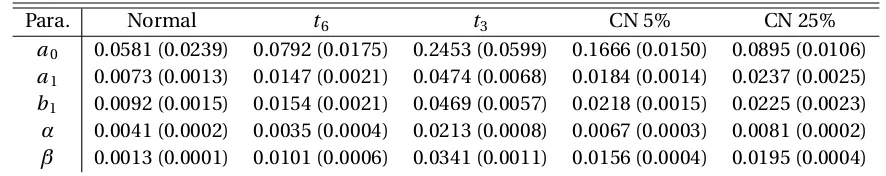
Table 4.1 Exchange Rate Volatility Parameter Estimation . . . 71
Table 4.2 ComparingR2Values of Q-Q Plots . . . . 74
Table 4.3 R2Combinations for Contaminated Normal . . . . 74
Table 4.4 Set 1 Results for Data Driven Comparison of Methods . . . 78
Table 4.5 Set 2 Results for Data Driven Comparison of Methods . . . 79
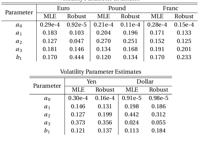
Table 4.6 Volatility Parameters Between Robust and Traditional Method . . . 80
Table 4.7 Correlation Parameters Between Robust and Traditional Method . . . 81
Table A.1 Complete MSE Results Across Generating Processes with First Portfolio . . . 97
Table A.2 Complete Bias Results Across Generating Processes with First Portfolio . . . 98
Table A.3 Complete Variance Results Across Generating Processes with First Portfolio . . . 99
Table A.4 Complete Results Across Generating Processes with Second Portfolio . . . 100
LIST OF FIGURES
Figure 1.1 Likelihoods ofα(a) andβ(b) without Split Likelihood Estimation . . . 5
Figure 1.2 Likelihoods ofα(a) andβ(b) with Split Likelihood Estimation . . . 6
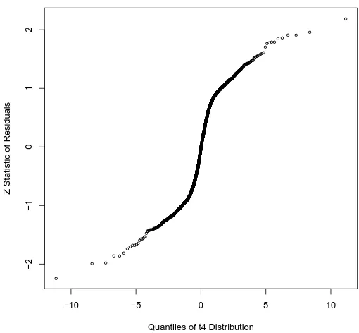
Figure 4.1 QQ-plot of Spherical Symmetry . . . 72
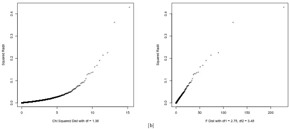
Figure 4.2 Q-Q Plots of Squared Radii withχ1.362 (a) andF2.75,3.48(b) . . . 75
Figure 4.3 Overlayed Estimated Volatility Time Plots . . . 82
Figure 4.4 Estimated Volatility Time Plots with[a]MLE and[b]Robust Estimation . . . 83
Figure 4.5 Overlayed Estimated Volatility Time Plots . . . 84
Figure 4.6 Time Plots of Determinant of Estimated Correlation Matrices . . . 86
Figure 4.7 Time Plots of Average Correlation Between Assets . . . 87
Figure B.1 Density Plots of Radii (a) and Squared Radii (b) . . . 104
Figure B.2 Estimated Volatility Time Plots of Euro (MLE[a], Robust[b]) . . . 105
Figure B.3 Estimated Volatility Time Plots of Pound (MLE[a], Robust[b]) . . . 106
Figure B.4 Estimated Volatility Time Plots of Franc (MLE[a], Robust[b]) . . . 107
Figure B.5 Estimated Volatility Time Plots of Yen (MLE[a], Robust[b]) . . . 108
Figure B.6 Estimated Volatility Time Plots of Dollar (MLE[a], Robust[b]) . . . 109
Figure B.7 Estimated Correlation Time Plots . . . 110
Figure B.8 Estimated Correlation Time Plots . . . 111
Figure B.9 Estimated Correlation Time Plots . . . 112
Figure B.10 Estimated Correlation Time Plots . . . 113
CHAPTER
1
Introduction
Volatility modeling plays a critical role in mathematical finance and statistical applications. The
ability to estimate and forecast volatilities for different assets and groups of assets leads to a better understanding of current and future financial risk. Many different methods of volatility estimation
have been developed over the past few decades. Understanding the characteristics of financial assets
helps develop estimation methods for volatilities. Studying volatilities of financial assets reveals that volatility seems to vary over time instead of remaining constant. The volatilities also exhibit some
persistence, or dependence over time, with a clustering effect of small (or large) number of returns
being followed by small (or large) number of returns of either sign. Letrt be the daily return of a financial asset, modeled byrt =
p
ht"t and"t as the random
error with the variance of 1. These daily returns are defined as the logarithm of the relative prices
log(Pt/Pt−1)withPt as the current time period price in dollars. It is reasonable to assume daily returns
have a conditional mean of approximately zero. This assumption is reasonable because an extremely
high annual return of 25% translates to a daily return of only 0.09%. Time weighted estimates are a reasonable initial guess of volatility estimation to account for persistence:
ht= n
X
i=1
ωirt2−i
withPni=1ωi =1 and the more recent observations more heavily weighted. A problem with this
approach is that many different weightsωi need defining. An exponential weight scheme where
ωi=λωi−1,withλbetween 0 and 1, potentially solves the problem. Other estimates have also been
1.1
ARCH
/
GARCH Volatility Modeling
Instead of a weighting scheme, Engle (1982) uses an autoregressive time series approach to account
for persistence in volatility estimation. He also assumes the conditional variance, or volatility, of returns varies over time. Engle’s autoregressive conditional heteroscedasticity (ARCH) model defines
the volatility as
ht=a0+a1rt2−1, (1.1)
witha0>0 anda1≥0 for the volatility to remain positive. Engle assumes the returns,rt givenψt−1,
follow a normal distribution:rt|ψt−1∼N(0,ht), whereψt−1represents all information up to time
t−1. This model easily extends toplags of returns with the ARCH(p) model
ht=a0+
p
X
i=1
airt2−i, (1.2)
witha0>0 andai ≥0 for alli. However, in practice, we often need large values ofp to accurately
model real world data.
Bollerslev (1986) avoids the problem of large values ofpin Engle’s ARCH model by generalizing the ARCH(p) model into the generalized autoregressive conditional heteroscedasticity (GARCH)
model, in much the same way as an autoregressive (AR) model extends to the autoregressive moving
average (ARMA) model. The GARCH model allows a longer memory process with more flexibility. The GARCH(p,q) model still assumes normality withrt|ψt−1∼N(0,ht), but instead of equation 1.2,ht is
defined as
ht=a0+
p
X
i=1
airt2−i+ q
X
i=1
biht−i, (1.3)
witha0>0,ai≥0, andbi ≥0. In many cases,p=q=1 is found to give an adequate fit. The univariate
ARCH/GARCH framework of models has been adapted into many different forms, which are detailed in Section 2.1.1.
The ARCH/GARCH framework of models also extends into a multivariate context, to model the
underlying volatilities and correlations between different market assets. The general multivariate extension to the GARCH model has a vector of assets as a stochastic processrt ofk×1 dimension
defined as
rt =H1t/2"t, (1.4)
whereH1t/2is a factor of the conditional variance-covariance matrix of sizek×k, and with Var("t) =Ik.
Bollerslev et al. (1988) modelHtas
where vech(·)is the operator that is a column-wise vectorization of the of the lower triangular portion
of a matrix, and the matricesAandBare parameter matrices. This specification of theHt matrix
is referred to as the VEC model. The number of parameters in this model grows very quickly as the number of assets in the model grows. To make parameter estimation feasible, Bollerslev, Engle, and
Wooldridge proposed to restrictAandBto diagonal matrices. Models with other specifications ofHt,
such as the BEKK(1,1,K) and Factor GARCH, are described in Section 2.1.2. Most of these approaches involve many parameters to be estimated, which leads to computational burdens for large portfolios
of assets.
A less computationally burdensome approach to multivariate GARCH estimation is a combination of univariate estimation of GARCH models and estimation of multivariate correlation matrices. This
greatly reduces the number of parameters by separately defining individual conditional variance
struc-tures and an overall correlation structure. Bollerslev (1990) designed one of these approaches with the constant conditional correlation GARCH (CCC-GARCH). The CCC-GARCH defines the conditional
covariance matrix of returns as
Ht =DtRDt, Dt=diag(
p
hi,t), (1.6)
whereRis a correlation matrix containing conditional correlations, andhi,t follows the univariate
GARCH model, defined as
hi,t=ai,0+
Pi X
p=1
ai,pri2,t−p+ Qi X
q=1
bi,qhi,t−q. (1.7)
The conventional sample correlation matrix is a reasonable estimate ofR. However, in practice the assumption that correlations of assets remain constant over time seems unrealistic. In particular, the constant correlations assumption understates risk if correlations increase in turbulent markets.
Engle (2002) relaxes the assumption of constant correlation in the dynamic conditional correlation
GARCH (DCC-GARCH) by allowing the correlation matrix to change over time. This model is widely used for its combination of computational ease as well as the evolving correlation matrix defined by
Ht=DtRtDt. (1.8)
Engle mentions two different estimates for theRt matrix. The first specification involves exponential
smoothing with
Qt = (1−λ)
"t−1"t0−1
+λQt−1, (1.9)
method uses a GARCH(1,1) model as a specification with
Qt=R0(1−α−β) +α("t−1"0t−1) +βQt−1, (1.10)
withR0as the unconditional correlation matrix andα+β <1.
This leads to the following specification of the DCC-GARCH model:
rt|ψt−1∼N(0,DtRtDt),
D2
t=diag(a0,i) +diag(a1,i)◦rt−1rt0−1+diag(b1,i)◦D2t−1,
"t=D−t1rt,
Qt=R0(1−α−β) +α("t−1"t0−1) +βQt−1,
Rt=diag(Qt)−1/2Qtdiag(Qt)−1/2,
(1.11)
where◦represents the elementwise product of the matrices. The log likelihood we would maximize to estimate the parameters of the model is
L=−1
2
T
X
t=1
nlog(2π) +2log|Dt|+rt0Dt−1D−t1rt−"t0"t+log|Rt|+"t0Rt−1"t
, (1.12)
as shown in detail in Appendix A. Maximizing this function over the parameters leads to the maximum
likelihood estimates (MLE) of the parameters. Engle suggests splitting the likelihood into the sum
of two parts to improve efficiency in calculating the model. The two components are the volatility component, which only depends on the individual GARCH parameters, and the correlation
compo-nent, which depends on both the correlation parameters and the individual GARCH parameters. Let
θ denote the volatility parameters in theDmatrix andφdenote the correlation parameters in theR
matrix. The split is written
L(θ,φ) =LV(θ) +LC(θ,φ), (1.13)
with the volatility part as
LV(θ) =−1
2
T
X
t=1
nlog(2π) +2log|Dt|+rt0Dt−1D−t1rt
, (1.14)
and the correlation part as
LC(θ,φ) =−1
2
T
X
t=1
log|Rt|+"t0Rt−1"t−"t0"t
. (1.15)
Engle first estimates the volatility parameters with ML estimation. He then places the estimates into
[a] ● ● ● ● ● ● ● ● ● ● ● ● ● ● ● ● ● ● ● ● ●
0.10 0.15 0.20 0.25 0.30
−2400 −2380 −2360 −2340 −2320 −2300 −2280 Alpha −Likelihood
[b]
● ● ● ● ● ● ● ● ● ● ● ● ● ● ● ● ● ● ● ● ● ● ● ● ● ● ●● ● ● ● ● ● ● ● ● ● ● ● ● ●
0.4 0.5 0.6 0.7 0.8
−2270 −2260 −2250 −2240 −2230 −2220 −2210 Beta −Likelihood
Figure 1.1: Likelihoods ofα(a) andβ(b) without Split Likelihood Estimation
After comparing estimates with both whole ML estimation and ML estimation across parts, the lack of efficiency mentioned above arises from problems in the estimation of the correlation parameters.
A set of three assets is evaluated with a DCC-GARCH model with correlation parametersα=0.24 and
β=0.7 over 500 periods in time with an initial correlation matrixR0defined as
1 0.85 0.85
0.85 1 0.85
0.85 0.85 1
.
A likelihood function of both theαandβparameters shows instability as shown in Figure 1.1. The graph of the likelihood functions above show the value of the likelihood function for changing values
of a single parameter as the other parameters in the model are held constant.
The instability in the estimation of these parameters poses a problem in trying to derive con-clusions about the model. The likelihoods for the correlation parameters show more stability when
imposing the technique of breaking the likelihood into two pieces, as seen in Figure 1.2. The immense improvement in the stability of the estimation of these parameters allows for better estimation of the
model parameters. With the split estimation technique, we can better examine the effects of outliers
in the maximum likelihood estimation of the DCC-GARCH.
1.2
Outliers and Robust Estimation
[a] ● ● ● ● ● ● ● ● ● ● ● ● ● ● ● ● ● ● ● ● ●
0.10 0.15 0.20 0.25 0.30
345 350 355 360 365 370 Alpha −final
[b]
● ● ● ● ● ● ● ● ● ● ● ● ● ● ● ● ● ● ● ● ● ● ● ● ● ● ●●● ● ● ●● ● ● ● ● ● ● ● ●
0.4 0.5 0.6 0.7 0.8
362 364 366 368 370 Beta final
Figure 1.2: Likelihoods ofα(a) andβ(b) with Split Likelihood Estimation
such as sample mean, sample variance, sample correlation, and regression modeling to estimate
parameters in the data. Many different robust estimation techniques have been used to estimate models from data when outliers are or are not present. Good robust estimates provide accurate
estimation of parameters in the presence or absence of outliers.
Outliers also affect maximum likelihood estimation (MLE). This is a common method of model pa-rameter estimation used in estimating the papa-rameters in the DCC-GARCH model. DefineL(β|yi, . . . ,yn)
as the log of the likelihood function for the random variableyi. We derive the MLE by solving either
ˆ
βMLE=arg max
β L(β|yi, . . . ,yn),
or taking the derivative of the log of the likelihood function and solving
n
X
i=1
`(β|yi) =0, (1.16)
where`(·)is the derivative of the log of the likelihood function. Under certain regularity conditions,
ˆ
βMLE is both consistent and asymptotically normally distributed. These maximum likelihood esti-mators are a specific subset of a general class of estiesti-mators called M-estiesti-mators developed by Huber (1964). These estimates,βˆψ, are solutions to
n
X
i=1
ψ(yi,β) =0, (1.17)
certain regularity conditions defined by Huber (1973),βˆis consistent and asymptotically normal.
Different choices of theψfunction lead to robust estimation of the parameters. These choices are
discussed further in Section 2.2.
It is beneficial to understand outliers in time dependent data because the DCC-GARCH model
uses an autoregressive structure in estimating the volatilities and correlations. Time series data, such
as financial data, contain greater potential for outliers hindering the estimation process, because of the underlying dependence between observations in the data. In time series data, outliers may occur
in patches throughout the data, or in isolation throughout the data. In some cases, entire shifts of
the process may occur. A couple of common outliers that may occur in time series data are additive outliers (AO) and innovation outliers (IO).
Maronna et al. (2006) describes additive outliers as outliers where instead of the expected
observa-tionyt, it is replaced byyt+υtwhereυt∼(1−ε)δ0+εN(µυ,σ2υ). In this definition,δ0is a point mass
distribution at zero and theσ2
υis significantly greater than the variance ofyt. This creates an outlier
with probabilityε, andnconsecutive outliers with probabilityεn. They defined innovation outliers
as outliers that affect both the current and subsequent observations. These outliers are especially
relevant in autoregressive (AR) and autoregressive moving average (ARMA) models.
Innovation outliers occur in the error term of the model. In this case, the observationyt is actually
affected, as shown with a simple AR(1) model:
yt=φyt−1+εt.
Ifεt comes from either a distribution with larger tails than a normal distribution or a mixture of two
normal distributions, thenyt becomes an outlier that directly affectsyt+1by
yt+1=φy¨t+εt,
where ¨yt is the value ofyt whereεt−1is not from a normal distribution. Both additive and innovation
outliers potentially bias the estimate along with changing the estimate’s variability.
Many different methods have been proposed to handle outliers in time series data, such as robust filter estimation for AR and ARMA models or M-estimation techniques both of which are described
in Maronna et al. (2006). These are just some of the different possible approaches, and more are
discussed in detail in Section 2.2.3. A robust filter approach replaces prediction residualsεˆt with
robust prediction residuals ˜εt by replacing outliers by robust filtered values. Instead of the typical
residual definition in an AR(p) model
ˆ
the new robust residuals are defined by
˜
εt= (yt−µ)−φ1(y˜t−1|t−1−µ)−. . .−φp(y˜t−p|t−1−µ),
where the ˜yi are a filtered prediction of the observation, which are approximations to the expected
value of that observation. The value ˜yt is equal toytif the value does not fall outside a predetermined
range from the expected value at that point. If ˜ytfalls outside the range, then the estimate is equal to
an approximation of the expected value at that point, given previous information. This robust filtering
approach extends into the ARMA class of models as well. Although this estimation works well for AO,
the process does not work as well in the presence of IO. M-estimation techniques for ARMA models minimize
T
X
t=p+1 ρ
ˆ
εt(β)
ˆ
σε
,
where theψappears in equation 1.17 may be the derivative of theρfunction appearing here,εˆtare the
model residuals, andσˆis a robust estimate of the standard deviation of the residuals. As mentioned
before, the M-estimation may be implemented using variousψfunctions, such as Yohai (1987) MM-estimate, to help limit effects of outliers. Yohai uses three steps for MM-estimation, where he first
computes an initial estimate ofβˆ. From this estimate, he computes a robust scale estimate,σˆ for the
residuals. He then uses an iterative process to continue the previous two steps until convergence. These estimates are relatively robust for contamination with AO, but lose their effectiveness as
the orderp of the AR(p) process increases. However, asymptotic theory for M-estimates is based on the assumption that the errors in the model are homoscedastic. The DCC-GARCH model is
heteroscedastic by construction. Although some M-estimates do not depend on homoscedastic
errors, they have lower efficiency than those that account for the lack of homoscedasticity.
An improved M-estimator without homoscedasticity takes into account the other covariates and
possible parameters making the errors heteroscedastic by
yt =β0xt+g(ξ,β0xt)εt,
whereξis a parameter vector limited to the error variance. To obtain robust estimates of both sets
of parameters, Maronna et al. (2006) suggest computing an initial estimate of the parameter vector
βby the proposed above MM-estimate. The residuals of this model are then calculated and used in the computation of an estimate of the parameter vectorξ. From here, robust transformations of the
originalyt andxtare calculated by dividing through by the estimatedg(·)function, to produce a more
parameters in the DCC-GARCH, but also the multivariate estimation of the correlation structure
between variables. The DCC-GARCH model requires the estimation of a covariance matrix to describe
the relationship between the multiple assets in the portfolio. White (1980) noted that heteroscedastic-ity not only hinders linear model parameter estimation, but also hinders covariance matrix estimation.
He proposes an estimate of the covariance matrix that is not unduly affected by the presence of
het-eroscedasticity and does not require a specific model of the hethet-eroscedasticity. He assumes that the errors in the model have heteroscedasticity of the formE(ε2
t|xt) =g(xt). Under some basic moment
assumptions of the errors in the model, White develops the estimator
ˆ Vn=
1
n
n
X
t=1
ˆ
ε2
t,MLEx
0
txt,
whereεˆt,M LE are the residuals evaluated with the parameters at the MLE values. Using the previous
estimator, the heteroscedasticity-robust covariance matrix is
ˆΣR=
x0
txt
n
−1
ˆ Vn
x0
txt
n
−1
. (1.18)
Outliers also affect covariance matrix estimation. Some proposed robust multivariate estimates of the covariance matrix are computationally burdensome in high dimensional data, such as some
financial data. Robust estimation of location and scale using Mahalanobis distances computed from
M-estimators are computationally difficult, according to Peña and Prieto (2001). They state that the minimum covariance determinant (MCD) by Rousseeuw (1984) is also computationally intensive. The
purpose of the MCD method is to takehobservations from the total that have the lowest determinant of the covariance matrix. The MCD estimate of the covariance matrix is just a multiple of these points’ covariance matrix. For this process to work, many iterations of resampling must take place, which
lead Rousseeuw and Van Driessen (1999) to create the FAST-MCD algorithm, explained in full detail in
Hubert et al. (2008).
Peña and Prieto again suggest that even the FAST-MCD algorithm requires too much resampling
and reduces heavy computation time with needed approximations. They suggest that outliers in
multivariate data created by a symmetric contamination tend to increase the kurtosis coefficient. The directions of the projected observations, based on kurtosis coefficients, lead to a better idea of which
directions contain outliers. They create an algorithm based on these projected kurtosis directions.
1.3
Summary
The above conclusions about the effects of outliers in autoregressive models, models with
het-eroscedasticity, and covariance matrix estimation, show the DCC-GARCH model is inherently hin-dered by outliers. This thesis proposes a robust estimation method for the DCC-GARCH that accounts
for outliers present in the data. The second chapter is a literature review of the explored papers and
topics in ARCH/GARCH modeling in both the univariate and multivariate context, robust estimation in univariate, multivariate, and time series data, previous attempts of ARCH/GARCH robust
estima-tions, and tests of symmetry for elliptical distributions. Chapter 3 proposes the robust estimation
method for the DCC-GARCH method and shows an example of outliers hindering the DCC-GARCH model while discussing the creation and asymptotics of the new robust estimation method. Chapter
4 discusses the attempts to identify real world data distributions for a data driven evaluation of the newly proposed model. Chapter 4 also summarizes the results of simulation studies comparing the
maximum likelihood fitting of the DCC-GARCH model with the newly proposed robust method, and
CHAPTER
2
Literature Review
This chapter reviews the past and current literature on univariate and multivariate ARCH/GARCH
modeling, robust estimation techniques, and tests of elliptical symmetry.
2.1
ARCH
/
GARCH Models
The following section will briefly revisit Engle’s ARCH model as mentioned in Section 1.1. Consider a random variablert drawn from a conditional distribution off(rt|ψt−1), whereψt−1is all information
up until timet−1. The current period forecast ofrt, after some basic assumptions, is the conditional
expected value given the previous period’s information, E(rt|ψt−1). Similarly, the variance of the
current period forecast is the conditional variance, Var(rt|ψt−1). However, traditional econometric
models did not take the previous period’s response ofrt−1into the calculation, by assuming
con-stant conditional variance. Engle (1982) proposed a model called the autoregressive conditional heteroscedasticity (ARCH) model, allowing the underlying forecast variability to change over time.
Modeling of heteroscedastic variances allows variances to change and evolve over time. Standard
heteroscedasticity corrections to predicting variances introduce an exogenous variablext to the
calculation as
rt ="txt−1
with E("t) =0 and Var("t) =σ2. This leads to Var(rt) =σ2xt2−1. Although this variance changes over
time, the variance depends on the changes of the exogenous variable instead of the possible evolution
Andersen (1978). This model allows the evolution of the conditional variance based on changes to the
response variable, but leads to an unconditional variance of either zero or infinity.
Engle’s ARCH model replaces the bilinear model with the following form
rt="th1t/2
ht=α0+α1rt2−1, (2.1)
with Var("t) =1. Engle assumes the normality ofrt given all of the information at the previous time
period,ψt−1, with
rt|ψt−1∼N(0,ht).
The ARCH model extends to an order ofp, with the ARCH(p) model only differing from the ARCH model through the function
ht =α0+ p
X
i=1
αirt2−i, (2.2)
with theαi’s restricted to positive values as defined in equation 1.2. Engle (1982) describes details of
the distribution of the ARCH process and importantly notes that the unconditional distribution of
the error possesses fatter tails than the normal distribution. Also, the ARCH(p) model possesses an
arbitrarily long lag structure when it is applied to real life data.
As mentioned in Section 1.1, Bollerslev (1986) corrects the problem of the arbitrarily long lag
structure of the conditional variance of the ARCH(p) model by generalizing the ARCH(p) model into
the general autoregressive conditional heteroscedasticity (GARCH) model. Bollerslev saw the long lag structure of the ARCH(p) model as potentially burdensome. The GARCH model still assumes
normality with
rt|ψt−1∼N(0,ht),
but instead ofht defined as in equation 2.2,ht is defined as
ht =α0+ p
X
i=1
αirt2−i+
q
X
i=1
βiht−i, (2.3)
withα0>0,αi≥0, andβi ≥0. The GARCH model withq=0 simplifies to an ARCH(p) model.
Bollerslev focuses on the simplest GARCH model, the GARCH(1,1) model. Bollerslev calculates the moments of the GARCH(1,1) model to find information about the distribution of the process. The
detailed calculations are found in Bollerslev’s paper, but the important finding is that the second and
fourth order moments exist and are given by
and
E(rt4) = 3α
2
0(1+α1+β1)
(1−α1−β1)(1−β2
1−2α1β1−3α21)
respectively, with the assumption of 3α21+2α1β1+β12<1 for the fourth moment to be finite. With
these two moments, the kurtosis of the distribution of the GARCH(1,1) process is
κ = E(rt4)−3E(rt2)2
E(r2
t)2
= 6α21(1−β12−2α1β1−3α 2 1)−
1.
Coupled with the assumption 3α21+2α1β1+β12<1, the excess kurtosis of the distribution is strictly
positive, which leads to a heavy tailed distribution. This is similar to the findings of Engle with the
ARCH process. Many extensions of the ARCH/GARCH framework have been proposed since their creation.
2.1.1 Extensions to Univariate ARCH/GARCH Models
Both ARCH and GARCH models may be used to account for the presence of volatility clustering in time
series such as financial data, where periods of high (or low) volatility are typically followed by further
periods of high (or low) volatility. Another typical aspect of financial data is that the unconditional distribution of the returns tends to have fatter tails than the normal distribution. Although ARCH and
GARCH models with conditional normal errors possess unconditional error distributions with fatter
tails than the normal distribution, the residuals in these models still often exhibit leptokurtosis. Some of the first extensions of the ARCH/GARCH modeling account for the leptokurtosis in the residuals of
these models.
Bollerslev (1987) proposes one of the first extensions of the ARCH/GARCH modeling system by making an adjustment to the conditional distribution of the error term. Bollerslev notes the usefulness
of the ARCH and GARCH models in portraying the clustering of volatilities in financial data. However,
he also notes that financial data are conditionally leptokurtic. Therefore, Bollerslev proposes to switch the conditional error distribution to at-distribution. The newt-distributed GARCH(p,q) he proposes is given by
rt|ψt−1 ∼ fν("t|ψt−1)
= Γ(ν+1
2 )Γ(
ν
2)
−1((ν
−2)ht)−1/2
×(1+"t2h−t1(ν−2)−1)−(ν+1)/2,
withν >2 andht defined in equation 2.3. Bollerslev estimates the degrees of freedom from the
cluster volatility aspects of the GARCH model and a higher leptokurtosis than the GARCH(1,1) with
conditional normally distributed errors.
Nelson (1991) notices three different problems with the GARCH model which Bollerslev proposes for asset pricing applications. Nelson notices that the GARCH model accounts for only the magnitude
of the volatility of the previous period and not whether the shift in volatility is up or down. This
goes against research that shows a negative correlation between present return and future return volatilities. He also notices the GARCH model is potentially too restrictive on the parameter estimates.
Lastly, Nelson shows that interpretation of volatility persistence in GARCH models is difficult. Nelson
proposes the Exponential GARCH (EGARCH) model, where the log of the volatilities is an asymmetric function of past returns given by
rt=h1t/2"t
log(ht) =α0+ q
X
i=1
αi(φεt−i+γ[|εt−i| −E(|εt−i|)]) + p
X
i=1
βilog(ht−i). (2.4)
Nelson considers a more general family of distributions for the error term instead of the normal
distribution. Nelson uses the Generalized Error Distribution (GED), which is normalized to have a
mean of zero and variance of one, for the error distribution. This normalized GED is given by
f(") = νe
−(1/2)|"/ν|ν
λ21+1/νΓ(1/ν)
λ≡
2−2/νΓ(1/ν)
Γ(3/ν)
1/2
,
withνa factor that determines the thickness of the tails of the distribution. Ifν=2, the error follows a normal distribution. For values ofν <2, the distribution has thicker tails than the normal. For values
ofν >2, the distribution has thinner tails than the normal distribution.
The EGARCH model possesses fewer restrictions on the parameters ofαi andβi. Therefore, if
αiφ <0, the model allows for asymmetry in the variances so the volatility tends to rise(or fall) when
εt−i is negative(or positive). Nelson notes that the EGARCH outperforms the traditional GARCH
model in asset pricing applications. Nelson also portrays the results of the EGARCH as easier to interpret than the traditional GARCH.
Jorion (1988) (see also Bollerslev et al. 1992) focuses his research on foreign exchange markets
and the examination of discontinuities in the data. Jorion believes that discontinuities in financial data lead to leptokurtosis in their unconditional distribution. Hopes of accounting for discontinuities
lead Jorion to combine jump-diffusion processes and ARCH models. He definesrt as the logarithm of
He proposes that prices follow a diffusion process given by
d Pt
Pt =α
d t+σd"t, (2.5)
which leads to a discrete time representation defined by
rt=µ+σ"t.
This model is equivalent to Engle’s structure ofrt with an included mean termµ.
However, this model does not account for discontinuities in the data. Therefore, Jorion alters
equation 2.5 into a mixed jump-diffusion model given by
d Pt
Pt =α
d t+σd"t+d qt, (2.6)
whered qt is a Poisson process characterized with a mean number of jumps with a jump size ofY per
unit of time. He assumes the size of the jumps has a lognormal distribution. With this alteration to
the process, the new function for returns is
rt =µ+σ"t+
nt X
i=1
log(Yi), (2.7)
wherent is the actual number of jumps occurring in the interval.
Jorion combines equation 2.7 with Engle’s ARCH(1) model defined in equation 2.1 to get the following model
rt =µ+h1t/2"t+
nt X
i=1
log(Yi)
ht=α0+α1(rt−1−µ)2. (2.8)
Jorion’s model accounts for discontinuities along with the clustering of volatilities present in financial
data. In comparison with the ARCH(1) model and the diffusion process, the jump-diffusion model
provides a lower Schwarz Criterion defined in Schwarz (1978). This points to the fact that the jump-diffusion process better represents the data compared to the other two models.
Hsieh (1989) agrees that the EGARCH specification can be better interpreted than the traditional
GARCH model. However, Hsieh compares the distributional extensions of Bollerslev, Nelson, and Jorion with his own extension in five different foreign exchange rate markets. Hsieh uses the EGARCH
model with four different conditional distributions. He compares Bollerslev’s traditional normal
following conditional distribution for the error term:
f(") =
Z∞
−∞
e1/4ξ21−1/2ξuφ
"e1/4ξ21−1/2ξu
φ(u)d u
Hsieh analyzes goodness of fit test statistics for each of the distributions. The goodness of fit test statistics reject the normal distribution for all five of the foreign exchange rates analyzed. However,
the goodness of fit test statistics do not reject only the normal log-normal mixture Hsieh proposes in
all of the models. The t-distribution and the normal-Poisson mixture distribution are not rejected in four of the currencies, while the GED is not rejected in only three of the currencies.
Engle et al. (1987) note that the conditional mean may also depend on the previous variances of
the data. Holding risky assets requires compensation that directly corresponds to the amount of risk in the assets. Engle, Lilien, and Robins develop the ARCH-in-Mean, or ARCH-M, model where the
conditional mean is a function of previous variances and possibly other covariates. The function of the returns is defined
rt =g(xt−1,ht;β) +h1t/2"t (2.9)
ht =α0+ p
X
i=1
αi(rt−i−g(xt−1,ht;β))2,
withg(·)commonly a linear or logarithmic function ofht andxt−1a vector of covariates. This model
allows a change in the variance of an asset to directly affect the price of the asset either positively or
negatively. The ARCH-M model accounts for financial theory that directly relates the trade-off of risk and return of assets. However, Bollerslev et al. (1992) note that consistency of the ARCH-M model
requires the correct specification of the model.
Engle and Bollerslev (1986) restructure the GARCH model specified in equation 2.3 to that of a stationary ARMA time series process. They rearrange the GARCH model to
rt2=
p
X
i=1
(αi+βi)rt2−i− q
X
j=1
βjvt−j+vt, (2.10)
wherevt=rt2−ht is a sequence of uncorrelated random variables. This model has the same
corre-lation structure as an ARMA(p,q) process with AR parameters(αi+βi)and the MA parameters−βj.
With the assumption ofp≥q, the above model is stationary ifPpi=1αi+
Pq
i=1βi≤1. However, Engle
and Bollerslev note the possibility of a unit root in the GARCH process whenPp
i=1αi+
Pq
i=1βi=1.
If the unit root is present, then the model becomes the Integrated GARCH (IGARCH) model. The
IGARCH(1,1) model is defined
which closely resembles a random walk model with drift because
E(ht+s) =sα0+ht.
Engle and Bollerslev mention the difficulties in testing for the presence of persistence in the IGARCH model.
2.1.2 Multivariate ARCH/GARCH Models
A multivariate framework leads to more applicable models compared to the univariate approach
when studying the relationships between volatilities in multiple assets at the same time. With a
multivariate approach, the multivariate distribution directly computes the implied distribution of portfolios compared to single assets. The specification of the multivariate GARCH model has a vector
stochastic processrtofk×1 dimension. Bauwens et al. (2006) define the process
rt=µt(θ) +H1t/2"t, (2.11)
whereH1t/2is the factor of thek×k positive definite matrixHt,"t as a white noise process, with the
mean of the error term equaling zero and the variance equalingIk. Many different specifications for
the conditional variance matrixHt are defined in this section.
Bollerslev et al. (1988) originally propose a formulation ofHt where each element of the covariance
matrix is a linear function of errors and lagged values of the elements ofHt defined as
vech(Ht) =c+Avech(εt−1ε0t−1) +Bvech(Ht−1). (2.12)
They call this the VEC(1,1) model. However, this model is highly parameterized in high dimensional systems, making the VEC(1,1) model hard to estimate. Also, the VEC model can not guaranteeHt is
positive definite. To help reduce the number of parameters, Bollerslev alters the VEC model into the
diagonal VEC (DVEC) model, which limitsAandBto diagonal matrices. This adaptation is still hard to estimate in high dimensional systems.
Also, Bollerslev et al. need additional conditions to ensure the conditional variance matrices are
positive definite. To ensure this, they assume that the matrices in equation 2.12 arec=vech(Co),
A=diag(vech(Ao)), andB=diag(vech(Bo)). They assume the matricesCo,Ao, andBo are positive
definite.
Engle and Kroner (1995) propose a solution to the positivity issues of the VEC and DVEC models with their BEKK(1,1,K) model. The BEKK model is a special case of the VEC class of models that
matrix as follows:
Ht =C∗0C∗+ K
X
k=1
A∗kεt−1ε0t−1A∗k+ K
X
k=1
B∗k0Ht−1B∗k (2.13)
The matrixC∗is limited to an upper triangular matrix. The BEKK model helps solve the positivity
issues of the VEC model, but still contains the difficulty in high dimensional parameter estimation. The BEKK model reduces the parameterizations of the VEC model only slightly. Therefore, the VEC
and BEKK models are not widely used for high dimensional estimation problems.
Kawakatsu (2003) details another approach to ensuring the positivity ofHt in the VEC model
without all of the parameter restrictions that the BEKK(1,1,K) model imposes. Kawakatsu proposes the
Cholesky factor GARCH that specifies a functional form in terms of the Cholesky factorization of the
conditional covariance instead ofHt. The advantage of the Cholesky factor GARCH is the assurance
that the conditional covariance is positive definite without imposing restrictions on the parameters
that do not identify the model.
The Cholesky factor GARCH specifiesLt from the decomposition ofHt−1/2=LtL0t as
vech(Lt) =c+ p
X
i=1
Aiht−i+ q
X
j=1
Bj"t−j, (2.14)
wherec,Ai,Bj are parameter arrays and the vech(·)is previously defined in Section 1.1. Since the
Cholesky factorLt of a positive definite matrix is not uniquely defined, we assume all the diagonal
elements ofLt are positive. This specification restricts the diagonal elements ofLt to depend on past
values of the diagonal elements and not past values of the innovation vector. Kawakatsu proposes
another specification ofLt as
vech(Lt) =c+ p
X
i=1
Aiht−i+ q
X
j=1
Bj|"t−j|.
The disadvantage of both these identification restrictions and the model in general is the parameters in the model become very hard to interpret.
Engle et al. (1990b) propose that a small number of underlying factors drive the common persis-tence in the conditional variances of the assets. The factor GARCH (F-GARCH) model by Engle et al.
(1990b) develop is a special case of the BEKK model defined in equation 2.13. Lin (1992) defines the
F-GARCH(p,q,K) model by
Ht = Ω + p
X
j=1
K
X
k=1
Ak jεt−1ε0t−1Aj k+
q
X
j=1
K
X
k=1
Bj k0 Ht−1Bj k (2.15)
αk jfkg0kandBk j =βk jfkgk0. With this specification,Ht is defined by
Ht= Ω + K
X
k=1
gkgk0
p
X
j=1
α2
k jfk0εt−jε0t−jfk+ q
X
j=1
β2
k jfk0Ht−jfk
.
There are also many different variants to the factor GARCH model in the literature.
2.1.3 Conditional Correlation Approach
Separately specified combinations of univariate GARCH model estimation and multivariate
correla-tion matrix estimacorrela-tion are a less computacorrela-tionally burdensome approach to estimating multivariate
GARCH models. This nonlinear combination approach greatly reduces the number of estimated parameters in the model.
Bollerslev (1990) proposes a model of this form, where the conditional correlation matrix remains
constant. As in equation 1.6, the constant conditional correlation GARCH (CCC-GARCH) model is defined as
Ht =DtRDt, Dt=diag(
p
hi,t),
whereRis a correlation matrix with conditional correlations andhi,tdefined as any univariate GARCH
model. The most basic GARCH representation is
hi,t=ai,0+
Pi X
p=1
ai,pri2,t−p+ Qi X
q=1
bi,qhi,t−q.
The matrixHt is positive definite if all the conditional variances are positive andRis positive definite.
The assumption that correlations of assets remain constant over time seems unreasonable in real world applications. Engle (2002) instead assumes a dynamic conditional correlation GARCH
(DCC-GARCH) model where the conditional correlation matrix changes over time. Section 1.1 describes Engle’s DCC-GARCH model in detail. The full specification of the DCC-GARCH model is
rt|ψt−1∼N(0,DtRtDt),
D2
t=diag(a0,i) +diag(a1,i)◦rt−1rt0−1+diag(b1,i)◦D2t−1,
"t=D−t1rt,
Qt=R0(1−α−β) +α("t−1"t0−1) +βQt−1,
Rt=diag(Qt)−1/2Qtdiag(Qt)−1/2.
the matrixRt as
Rt = (1−θ1−θ2)R0+θ1Rt−1+θ2Ψt−1,
where the elements ofΨt are defined as
ψi j,t−1=
PM
h=1"i,t−h"j,t−h
q
PM
h=1"
2
i,t−h
PM
h=1"
2
j,t−h
.
Therefore,ψt−1is the sample correlation matrix of an M length rolling window of previous time points.
To guaranteeΨt is positive definite, place the restrictionM≥K.
Audrino and Barone-Adesi (2006) notice that Engle’s DCC-GARCH model constrains the
correla-tion dynamics to be equal across all of the assets. Audrino and Barone-Adesi relax this assumpcorrela-tion
in the creation of the average conditional correlation GARCH (ACC-GARCH) model. They propose their model as another approach to extend Bollerslev’s CCC-GARCH. The ACC-GARCH has the same
functional form as the other conditional correlation approaches with the volatility and correlation
structures defined separately. The univariate volatility portion of the model is similarly defined by any univariate GARCH model; the authors use the GARCH(1,1) structure defined by
ht =α0+α1rt2−1+β1ht−1.
Again, the main difference between the ACC-GARCH and other conditional correlation models is the
form of the correlation matrixRt. Audrino and Barone-Adesi define the correlation matrixRt as
Rt= (1−λ)Q t−1
t−p+λRt, λ∈[0, 1],
whereQtt−−1p is defined as the unconditional correlation matrix of the returns over the pastpdays. The matrixRt is a matrix with ones on the diagonal and all other elements equal to
rt=
1
k−1
k
k
X
i=1
k
X
j=1
σt,iσt,j
Pk
d=1σt,d
2−1
,
wherek is the number of assets in the portfolio. When the parameterλis zero, the model becomes very similar to the CCC-GARCH with a rolling window correlation estimate. The ACC-GARCH model
is estimated similarly to the two stage estimation of Engle’s DCC-GARCH with the details not included here. The detail of the nonparametric procedure is left to Audrino and Barone-Adesi (2006).
Pelletier (2006) develops a regime switching model as a balance between Bollerslev’s CCC-GARCH
constant within a regime and changes across different regimes. The RSDC model uses a Markov
chain to switch between the regimes. Pelletier still takes the foundational approach of Bollerslev in
equation 1.6 withrt =H1t/2"t, but defines the matrixHt as
Ht =StΓtSt (2.16)
whereSt is a diagonal matrix composed of standard deviations andΓt is a correlation matrix. The
correlation matrixΓt is defined as
Γt= N
X
n=1
1∆t=nΞn
with1representing the indicator function,∆t an unobserved Markov chain process that is
inde-pendent of"t,Ξnare correlation matrices, andN is the total number of regimes. The Markov chain
process∆t can take integer values from 1 toN. Pelletier imposes constraints on the matricesΞn
to ensure thatΓt is a correlation matrix. He works with the Cholesky factorizationΞn =PnPn0 and
imposes constraints onPnto makeΞnpositive definite.
A benefit of Pelletier’s RSDC model over the DCC-GARCH models of Engle and Tse and Tsui is that
the RSDC model allows for computation of multi-step ahead conditional expectations of the variance matrix. This is due to the linearity of the correlation model from the Markov chain. DCC-GARCH
models use square roots of variances that input nonlinearities in the model. Furthermore, Pelletier
defines the volatility standard deviations with the ARMACH model of Taylor (1986) and Schwert (1989) to perform these calculations for the entire variance matrix. The ARMACH model defines the standard
deviations in the volatility portion of the model as
st=α0+ p
X
i=1
αi|rt−i|
E|"˜t| +
q
X
i=1
βist−i (2.17)
This model may include a more robust approach to estimating volatility by the use of absolute
deviations of returns instead of squared returns. The ARMACH model is not required by the RSDC
model but does allow for the computation of multi-step ahead conditional expectations of the entire variance matrix. Pelletier (2006) gives further details of the estimation of the parameters in the RSDC
model.
2.2
Generalized Robust Estimation
Generalized linear models (GLM) defined by Nelder and Wedderburn (1972) play a prominent role in
the field of statistics. Generalized linear models have the following joint density:
The conditional density of the response variable vectorY given the explanatory variable vectorX=x
isf∗(Y;XTβ), which depends on the unknown parameter vectorβ. The marginal density ofXisu(X)
in the above equation.
Let(yi,xi)fromi=1, . . . ,nbe independent observations fromf∗(Y,X;β). Under certain regularity
conditions, the maximum likelihood estimator (MLE)βˆMLE, is the solution to
n
X
i=1
`(yi,xi,β) =0, (2.19)
with`(·)being the derivative of the log of the likelihood function. Under further regularity conditions,
ˆ
βMLE is both consistent and asymptotically normally distributed.
A few anomalous observations can strongly affect the MLE. These anomalous observations, or outliers, can come in two common forms - leverage points and residuals. A leverage point occurs
when a pointxi is an outlier in the covariate space. For example, ifxi is an outlier in the covariate
space, thenzi= (yi,xi)is a leverage point. These leverage points are either harmful or not, depending
on whether the error ofzi is large or small, respectively. Another type of outlier is a vertical outlier that
occurs when a pointzi is not a leverage point but still has a large residual, as described in Croux and
Haesbroeck (2003). These different types of outliers lead to different problems with the generalized linear model.
Anomalous observations should not affect robust estimators to the extent that they affect the
MLE. These robust estimators should be approximately equal to the parameters even in the presence of outliers. The addition or deletion of a few observations should not greatly affect the parameter
estimates or analysis in robust estimation.
Multiple approaches to robust estimation of parameters in generalized linear models have been
developed over the past few decades. Some of the first approaches to solving the problems with robust
estimation in GLM involve a notion of the sensitivity of an estimator. Robust estimators should not be as sensitive to changes in small numbers of observations. This would ensure that one observation
being an outlier would not greatly affect the estimated parameter. Creating a specific measure of
sensitivity permits the comparison of different estimators. Bounding this measure of sensitivity would then ensure that an estimator could not have an infinitely large sensitivity. Call the function
Ωthe influence function, whereΩ(yi,xi)represents the effect of a single observation(yi,xi)on the
estimation. Bounding this influence functionΩis a form of bounding the sensitivity of the estimator as mentioned in Hampel (1974). The focus here turns to the influence of the class of estimators called
M-estimators defined in equation 1.17. From Stefanski et al. (1986), the influence function of an
M-estimator is
Ω(yi,xi) = ψ(
yi,xi;β)
−(∂ /∂ β)E(ψ(yi,xi;β))
,
bounding the influence function would not only ensure relative efficiency, but also ensure robustness
of the estimator because any observation would have a limited effect on the estimator.
2.2.1 Break-down Point Approach
Instead of trying to measure the sensitivity of an estimator with influence functions, another approach
is to measure the amount of outliers in the sample it would take to ruin the estimate. Since every sample is of different size, an exact number of outliers to ruin the estimator would not be helpful, but
a percentage of observations that are potential outliers is understandable for any sample size. The
break-down point is the maximum percentage of outliers in a sample before the estimator becomes completely inaccurate.
Yohai (1987) notes that most robust estimators of the time had extremely low break-down points.
Therefore, even if the estimators are robust by definition, it would only take a small percentage of outliers in the sample to ruin even the robust estimator. Yohai points out that Huber’s M-estimation
even had a break-down point of zero. Rousseeuw and Yohai (1984) propose a method that tries to
keep the flexibility and asymptotic properties of the M-estimators, but has a higher breakdown point. Rousseeuw and Yohai focus their attention on estimating the scale of the residuals to derive their
parameter estimates in the regression model
yi=xiTβ+ξi.
They define a symmetric and continuously differentiable functionρwhere there exists a positive
constantc such thatρis strictly increasing on[0,c]. They defined the scale estimates,s, as the solution to the equation
1
n
n
X
i=1 ρ
ˆ
ξi
s(β)
=Eρ(ˆξ), (2.20)
whereξˆi=yi−xiTβ. The S-estimator,βˆS, is the solution of
arg min
β s(ˆξ1, . . . ,ξˆn). (2.21)
Rousseeuw and Yohai propose a possible functionψ=ρ0defined as Tukey’s biweight function
ψ(k) =
kh1−kc2i2 if|k| ≤c
0 if|k|>c
,